Present Address: ]Simplex Holdings, Inc., 19F Toranomon Hills Mori Tower, 1-23-1 Toranomon, Minato-ku, Tokyo 105-6319, Japan; [email protected]
Theory of rigidity and numerical analysis of density of states of two-dimensional amorphous solids with dispersed frictional grains in the linear response regime
Abstract
Using the Jacobian matrix, we obtain theoretical expression of rigidity and the density of states of two-dimensional amorphous solids consisting of frictional grains in the linear response to an infinitesimal strain, in which we ignore the dynamical friction caused by the slip processes of contact points. The theoretical rigidity agrees with that obtained by molecular dynamics simulations. We confirm that the rigidity is smoothly connected to the value in the frictionless limit. For the density of states, we find that there are two modes in the density of states for sufficiently small , which is the ratio of the tangential to normal stiffness. Rotational modes exist at low frequencies or small eigenvalues, whereas translational modes exist at high frequencies or large eigenvalues. The location of the rotational band shifts to the high-frequency region with an increase in and becomes indistinguishable from the translational band for large .
I Introduction
Amorphous materials consisting of dispersed grains such as powders, colloids, bubbles, and emulsions are ubiquitous in nature Jaeger96 ; Durian95 ; Wyart05 ; Baule18 . These materials behave like liquids at low densities and exhibit solid-like mechanical responses above their jamming point Liu98 . In systems consisting of frictionless grains, the rigidity changes continuously, but the coordination number of grains changes discontinuously at the jamming point as a function of density Durian95 ; Wyart05 ; Hern03 . The critical behavior near the jamming point is of interest to physicists as a non-equilibrium phase transition Hern01 ; Trappe01 ; Zhang05 ; Majmudar07 ; Ciamarra11 . Dispersed grains above the jamming point are fragile and exhibit softening and yielding transition under certain loads Nagamanasa14 ; Knowlton14 ; Kawasaki16 ; Leishangthem17 ; Bohy17 ; Ozawa18 ; Clark18 ; Boschan19 ; Singh20 ; Otsuki21 .
For amorphous solids consisting of frictionless grains, it is useful to analyze the dynamical matrix or the Hessian matrix, which is defined as the second derivative of the potential of a collection of grains with respect to the displacements from their stable configuration Wyart05 ; WyarLettt05 ; Ellenbroek06 ; Lerner16 ; Gartner16 ; Bonfanti19 ; Baule18 . For instance, the rigidity can be determined by eigenvalues and eigenvectors DeGiuli14 ; Mizuno16 ; Maloney04 ; Maloney06 ; Lemaitre06 ; Zaccone11 . It has been reported that the minimum nonzero eigenvalue of the Hessian matrix decreases with increasing strain and eventually becomes negative, where an irreversible stress drop takes place Maloney04 ; Maloney06 ; Manning11 ; Dasgupta12 ; Ebrahem20 .
It is known that amorphous solids have characteristic properties at low temperatures (e.g., thermal conductivity and specific heat) that are quite different from those of crystalline solids since a long-time ago Zeller71 . These days, we have recognized that amorphous solids consisting of dispersed grains exhibit unique elastic-plastic behavior as a mechanical response to an applied strain Nicolas18 . Because these properties are related to the density of states (DOS), there have been lots of studies on the DOS Hern03 ; Schirmacher07 ; Lerner16 ; Mizuno17 ; Wang19 . The DOS for systems composed of anisotropic grains, such as ellipses, dimers, deformable grains, and grains with rough surfaces, have been studied with the aid of the Hessian matrix Zeravcic09 ; Mailman09 ; Schreck10 ; Yunker11 ; Schreck12 ; Shiraishi19 ; Papanikolaou13 ; Britoa18 ; Treado21 ; Ikeda20 ; Ikeda21 . Because of the rotation of such anisotropic grains, there exists a rotational band in the DOS that is distinguishable from the translational band Mailman09 ; Yunker11 ; Schreck12 ; Britoa18 ; Ikeda20 ; Ikeda21 .
Even for systems of spherical grains that cannot be free from inter-particle friction, similar results are expected as a result of grain rotations. However, few studies have reported the existence of rotational bands in the DOS. Because the frictional force between the grains depends on the contact history, it cannot be expressed as a conservative force. Therefore, stability analysis for frictional grains based on the Hessian cannot be used. Nevertheless, the Hessian analysis using an effective potential for frictional grains has been performed Somfai07 ; Henkes10 . Recently, Liu et al. suggested that the Hessian analysis with another effective potential can be used even if slip processes exist Liu21 . The previous studies Somfai07 ; Henkes10 reported that friction between grains causes a continuous change in the functional form of the DOS from that of frictionless systems. However, there are only a few reports on whether an isolated band in the DOS originating from friction between grains is visible at lower frequencies.
Recently, Chattoraj et al. discussed the stability of the grain configuration under strain using the Jacobian matrix of frictional grains Chattoraj19 . They performed eigenvalue analysis under athermal quasi-static shear processes and determined the existence of oscillatory instability originating from inter-particle friction at a certain strain Chattoraj19 ; Chattoraj19E ; Charan20 . However, they did not discuss the rigidity or the DOS.
The theoretical determination of the rigidity of amorphous solids consisting of frictional grains is important for controlling amorphous solids. However, we do not know how to determine the rigidity from the Jacobian for the frictional grains.
The purpose of this study is to clarify the role of mutual friction between grains in terms of the rigidity and DOS. We focus on the response to an infinitesimal strain from a stable configuration of grains without any strain to obtain tangible results. In this study, we assume that there is no slip between grains because of an infinitesimal strain, and we then deal with friction as static friction.
The remainder of this paper is organized as follows. In the next section, we introduce the numerical method. In Sec. III, we introduce the Jacobian. Section IV consists of Sec IV.1, which deals with the theoretical prediction of rigidity in the linear response regime, and Sec. IV.2, which deals with the DOS. In the final section, we summarize the results of our study and discuss future work. The appendix consists of seven sections. In Appendix A, we summarize the method for preparing a stable grain configuration before applying shear. In Appendix B, we explain the implementation of the numerical integration method in the proposed system. In Appendix C, we summarize some properties of the Jacobian. In Appendix D, we present the explicit expressions of the Jacobian. In Appendix E, we investigate the effects of rattlers. In Appendix F, we write down the explicit results of Jacobian. In Appendix G, we derive the theoretical prediction of rigidity using the Jacobian. In Appendix H, we introduce the DOS using the Hessian analysis. In Appendix I, we investigate the system size dependence of the DOS. In Appendix J, we study the density dependence of the DOS.
II Numerical model
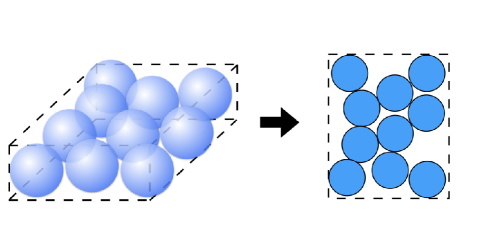
Our system contains frictional spherical particles embedded in a monolayer configuration. We treat this system as a two-dimensional system (see Fig. 1).
To prevent the system from crystallizing Luding01 , we prepare an equal number of particles with diameters and . We assume that the mass of particle is proportional to , where is the diameter of -th particle. We introduce as the mass of a particle with diameter . In this study, , and denote coordinates, and the rotational angle of the -th particle, respectively. We introduce the generalized coordinates of the -th particle with and , where the superscript T denotes the transposition.
Let the force, and -component of the torque acting on the -th particle be and , respectively. Then, the equations of motion of -th particle are expressed as
| (1) | ||||
| (2) |
with the mass and the momentum of inertia of -th particle. In a system without volume forces such as gravity, we can write
| (3) | ||||
| (4) |
where and are the force and -component of the torque acting on the -th particle from the -th particle, respectively. Here, is given by
| (5) |
where we have introduced the normal unit vector between and particles as . Here, and refer to -components of and , respectively. Note that expresses or throughout this study. The force can be divided into normal and tangential parts as
| (6) |
where and is Heaviside’s step function, taking for and otherwise. We model the repulsive force between the contacted particles and as the Hertzian force in addition to the dissipative force proportional to the relative velocity with a damping constant Liu21 as follows:
| (7) | ||||
| (8) |
where and are the stiffness parameters of normal and tangential contacts, respectively. For the normal compression length and its velocity are denoted as and respectively. For the tangential deformation, with the aid of , the tangential velocity is defined as , where we have introduced
| (9) |
with and . Here, and is the integration over the duration time of contact between and particles. Although the dissipative force between grains interacting with the Hertzian force is proportional to the product of the relative velocity and Kuwabara87 ; Brilliantov96 ; Morgado97 , we adopt simple dissipative forces as in Eqs. (7) and (8) because we are not interested in the relaxation dynamics. We note that Eqs. (7) and (8) assume the Hertzian contact force for the static repulsion of contacting spheres, but all calculations in this study are those for two-dimensional systems. Here, we do not consider the effects of slips in the tangential equation of motion. This treatment can be justified if we restrict our interest in the linear response regime to a stable configuration of particles without any strain. This situation corresponds to frictional grains with infinitely large dynamical friction constant, in which the friction is only characterized by static friction. Therefore, our analysis does not apply to systems with finite strain Otsuki17 , where the effect of slip is important.
To generate a stable configuration of frictional particles, we prepare a stable configuration of frictionless particles in a square box of linear size using a fast inertial relaxation engine (FIRE) Bitzek06 . Subsequently, we turn on the tangential force using Eqs. (1) and (2) to achieve a stable configuration in the force-balanced (FB) state for frictional particle111 For simplicity, we prepare the configuration before applying shear for frictionless particles at first, and then considered the friction between particles. If we prepare a configuration before applying shear by compressing frictional particles, we confirm that the configuration had an oscillatory instability that resulted from the appearance of a pair of imaginary eigenvalues of the Jacobian divided by mass matrix: Chattoraj19 ; Chattoraj19E ; Charan20 , where , and are the complex, real, and imaginary eigenvalues of , respectively. Here, is the Jacobian defined in Eq. (18), and is the mass matrix whose explicit form is given by , where . Because the linearized equation of motion is expressed as , there are four fundamental solutions , where consists of and . Here, and satisfy the relation . Thus, to avoid the oscillatory instability of the configuration before applying shear, we adopt the protocol of creating the configuration with frictionless particles, and then let the system relax by adding static friction between particles. (see Appendix A for details). Here, the FB state satisfies the FB conditions and for arbitrary particles. Note that we set when the tangential force is turned on.
We impose the Lees-Edwards boundary condition Lees72 ; Evans08 , where the direction parallel to the shear strain is -direction. After applying a step strain to all particles, -coordinate of the position of the -th particle is shifted by an affine displacement , where the superscript FB denotes the FB state. The system is then relaxed to the FB state by the contact forces between the particles expressed in Eqs. (7) and (8). Here, -components of translational and rotational nonaffine displacements of the -th particle after the relaxation process are, respectively, defined as
| (10) | ||||
| (11) |
Using Eqs. (10) and (11), we introduce the rate of nonaffine displacements as:
| (12) | ||||
| (13) |
Our system is characterized by the generalized coordinate . The configuration in the FB state at strain is denoted as . The shear stress at for one sample is given by:
| (14) |
The rigidity in the linear response regime for one sample is defined as
| (15) |
where the differentiation on the right-hand side (RHS) of Eq. (15) is defined as follows:
| (16) |
In the numerical calculation, we use a non-zero but sufficiently small for the evaluation of . Then, the rigidity in the linear response regime is defined as
| (17) |
where is the ensemble average.
For the numerical FB condition, we use the condition for arbitrary , where is the threshold force for the simulation and is the generalized force, defined as .
In our simulation, we adopt and . The control parameters are the ratio of the tangential to normal stiffness and projected area fraction to two-dimensional space . The operating ranges of and are to and to , respectively. In this study, we mainly present the results for and with the ensemble averages of samples for each and . Some results are obtained with , , and five samples for each and . We verify that the results are independent of the choice of for . We ignore the effect of dissipation between particles because the velocity of each particle is sufficiently small for infinitesimal agitation from the FB state. The time step of the simulation, , was set to , and numerical integration was performed using the velocity Verlet method (see Appendix B), where . To obtain eigenvalues and eigenvectors of the Jacobian matrix, which will be introduced in detail in the next section, we have used the LAPACK, which provides a template library for linear algebra.
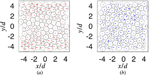
Figure 2 (a) shows an example of the affine displacements of particles, where the displacements exist only in the shear direction, and Fig. 2 (b) shows the nonaffine displacements.
III Theoretical Analysis
In this section, we introduce the Jacobian, the DOS, and theoretical expressions of the linear rigidity. Here, we omit the effects of because the dissipative term proportional to vanishes under quasistatic shear.
III.1 Jacobian and the DOS for frictional particles
In frictional systems, the stability of the system and DOS at are analyzed using the Jacobian () defined as Chattoraj19 :
| (18) |
where and are any of and , while and express particle indices. Therefore, the Jacobian matrix, which is a matrix, can be written as
| (19) |
where is a submatrix of the Jacobian for a pair of particles and :
| (20) |
See Appendices C and D for detailed properties of the Jacobian. The right and left eigenvalue equations of are, respectively, given by
| (21) | ||||
| (22) |
where and are the right and left eigenvectors corresponding to , respectively. Here, is the -th eigenvalue of . Note that and satisfy the orthonormal relation with normalization , if all eigenstates are non-degenerate. Here, the inner products for the right and left eigenvectors are defined as and , respectively. In the presence of friction, the eigenvalue is generally a complex number, but if we restrict our interest to infinitesimal distortions from stable configurations without shear strain, becomes real and can be expressed as . The DOS is the distribution function of the eigenvalues, defined as:
| (23) |
where on RHS of Eq. (23) expresses that the summation excludes the contribution of rattlers (see Appendix E for the details of rattlers). Using the force decomposition, the Jacobian can also be divided into
| (24) |
where
| (25) | ||||
| (26) |
for and
| (27) | ||||
| (28) |
for . Here, we have introduced and , where and are -component of and , respectively. Note that denotes the summation for contacted particles of the -th particle. The explicit expressions of and are presented in Appendix F
III.2 Expressions of the linear rigidity via eigenmodes
Let us introduce as
| (29) |
Because the forces acting on the particles are balanced in the FB state, satisfies
| (30) |
where is the ket vector containing for all components. The stable configuration in the FB state satisfies
| (31) |
where
| (32) |
Introducing
| (33) |
the left-hand side (LHS) of Eq.(31) can be rewritten as:
| (34) |
where we have used Eqs. (12) and (13) (see Appendix G.1). The first and second terms on RHS of Eq. (34) represent the strain derivatives of the forces for the contributions from the affine and nonaffine displacements, respectively. The explicit form of is given by:
| (35) |
Note that the tangential displacements do not contribute to . This is because the affine displacements are applied to our system instantaneously as a step strain; thus, the integral interval of the tangential displacement during the affine deformation is zero. We have used in Eq. (34) defined as
| (36) |
and
| (37) |
for .
Expanding the nonaffine displacements by the eigenfunctions of and using the fact that the LHS in Eq. (34) is zero, we obtain
| (38) |
where , and are the -th eigenvalue of , and the left and right eigenvectors corresponding to , respectively. Note that and satisfy the orthonormal relation , if all eigenstates are non-degenerate. See Appendix G.1 for the derivation of Eq. (38).
The rigidity in the linear response regime under infinitesimal strain is decomposed into two parts:
| (39) |
where and are the rigidities corresponding to the affine and nonaffine displacements, respectively. With the aid of Eqs. (14), (17), and (37) the expressions of and are, respectively, given by (see Appendix G.2)
| (40) | ||||
| (41) |
where we have introduced
| (42) | ||||
| (43) |
IV Results
In this section, we present the results of eigenvalue analysis and rigidity based on the formulation explained in the previous section. In Sec. IV.1, rigidity is determined using the eigenmodes of the Jacobian. Section IV.2 clarifies the effects of translational and rotational motions on the DOS.
IV.1 Theoretical evaluation of
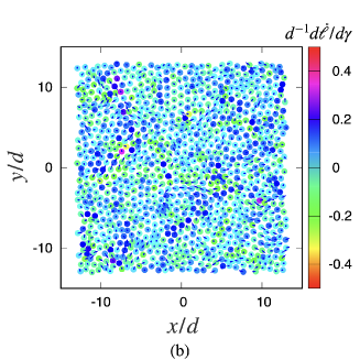
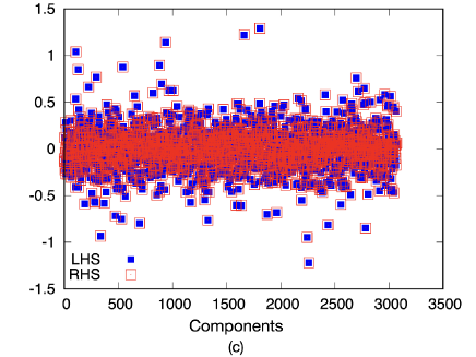
In this subsection, the validity of the theoretical rigidity presented in the previous section is demonstrated. For this purpose, at first, we examine the validity of Eq. (38), obtained by the eigenfunction expansion of the nonaffine displacements for RHS and by the simulation for LHS. Figures 3 (a) and (b) illustrate the nonaffine displacements on LHS and RHS of Eq. (38), respectively. In Figs. 3 (a) and (b), and -components of at are represented by vectors and colors, respectively. Figure 3 (c) shows the RHS and LHS of Eq. (38) against the components of the vectors whose orders follow Eq. (33), that is, the local order of the component follows and by fixing the particle number, and we align the components from the first particle to the -th particle without omitting modes with extremely small and zero eigenvalues. Figure 3 shows that the expression in Eq. (38) correctly reproduces the simulation results.

The dimensionless rigidity obtained from Eqs. (39),(40) and (44) with the aid of is shown in Fig. 4. This indicates the quantitative agreement between the theoretical and numerical values.
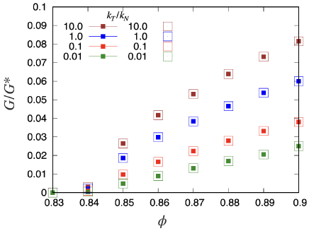
Therefore, the rigidity in the linear response regime can be determined completely using the Jacobian analysis. On the contrary to the previous studies Hern03 ; Olsson11 ; Otsuki11 , we should note that is not proportional to for a large , where is the critical fraction of jamming transition for frictional grains.
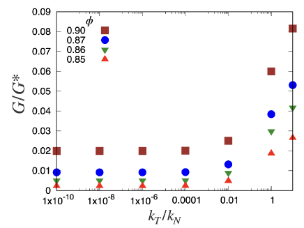
As is expected, the rigidity depends on only little for (see Fig. 5), while depends on for . We have confirmed that smoothly approaches the frictionless value in the limit in contrary to Refs. Otsuki17 ; Ishima20 . Here, cannot be expressed as a factorization for large 222 We have confirmed that the factorization is not held, where is the rigidity of frictionless system. . When we consider the effect of the dynamical friction, that is, slips between particles, the rigidity is discontinuously changed in the frictionless limit Otsuki17 ; Ishima20 . However, the rigidity continuously changes with in our system and is smoothly connected to that of frictionless systems (). Because our system can be regarded as having infinitely large static and dynamical frictional constants, there is no slip between the grains. Therefore, it might be natural for to continuously change the limit for in our system. In future work, we will consider the effects of slips, which are important for real frictional grains.
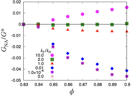
To clarify the contributions of nonaffine deformations to the rigidity, we plot defined in Eq. (41) against in Fig. 6, in which becomes large as increases. Remarkably, is positive for , at , and is negative for . The positive for a large is counterintuitive, in which increases from even when the system is relaxed to the FB state. In the future, we must clarify the origin of this counterintuitive . We note that the negative for a small can be understood by the relaxation process to look for a FB configuration after applying affine deformations to the system.
IV.2 Analysis of eigenvalues and eigenvectors
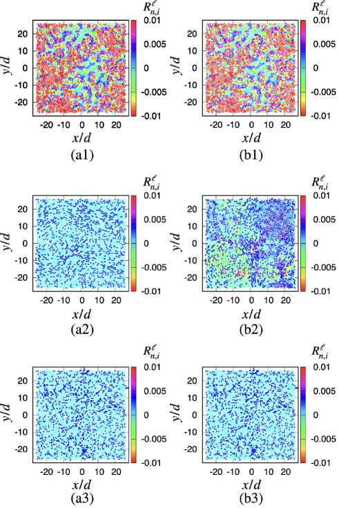
In Fig. 7 we present some typical right eigenvectors , which was introduced in Eq. (21), and can be expressed as:
| (48) |
where . Figure 7 illustrates vectors and colors to characterize the rotation of particle for some characteristic with (Figs. 7 (a1)-(a3)) and (Figs. 7 (b1)-(b3)). Figures 7 (a1) and (b1) show the eigenvectors at and , respectively, which are dominated by the rotational modes. In Fig. 7 (a2), we confirm that the eigenvector at is expressed only by translational modes, whereas the eigenvector at shown in Fig. 7 (b2) is expressed as a coupling mode of the rotational and translational modes. In Figs. 7 (a3) and (b3), we show the eigenvectors at which are dominated by the translational modes.
To clarify the translational and rotational contributions at each eigenvalue, we compute the translational and rotational participation fractions Yunker11 ; Shiraishi19 defined as
| (49) | ||||
| (50) |
respectively, where we have investigated the localization of the system with the participation ratio in Appendix E. Note that translational mode is dominant when is close to and rotational mode is dominant when is close to . and are plotted for various in Fig. 8, where
| (51) | ||||
| (52) |
Here, and are set to zero if there is no right eigenvalue for with the -th data point . Here, we have used the following steps to determine each data point. First, we divided the data interval into parts on a logarithmic scale. Then we linearly re-divided the data interval from the highest frequency to the 10th highest frequency region. Finally, we also linearly re-divided the data interval of the log scale corresponding to . Note that for the linear re-division of the data, the regions were divided into or equally spaced inter-regional intervals for high frequency or , respectively.
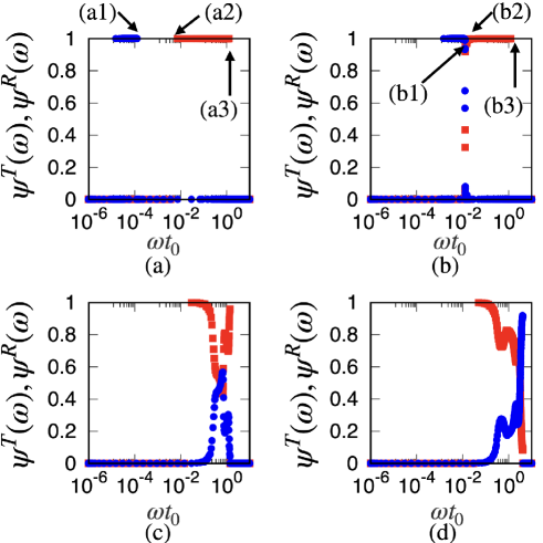
As shown in Figs. 8 (a) and (b), we find the region of for low and . This region is referred to as Region I. We also find a region that satisfies for high and , in which the translational modes are dominant. This region is referred to as Region II. Here, three characteristic behaviors depend on at . First, the translational modes are separable from the rotational modes for because we need a small amount of energy to excite the rotational mode in nearly frictionless situations, as shown in Figs. 8 (a) and (b). Second, the translational and rotational contributions are not separated for . Third, the translational and rotational contributions are indistinguishable for .
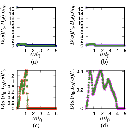
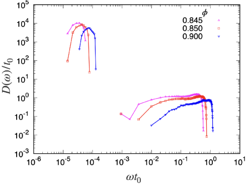
The DOS obtained from the Jacobian eigenvalues is shown in Fig. 9. Based on the results of and , the DOS is also separated into two regions for . The rotational band for low shifts to the high region as increases (see Figs. 9 (a) and (b)). In Region II with a high (see Figs. 9 (a) and (b)), the DOS is almost independent of in which the translational modes are dominant for . The distinctions between the two regions for the DOS are visible with a distinct gap between the adjacent regions for . For ; however, the high region of the DOS in Region I partially overlaps with the low region of Region II. Furthermore, Regions I and II are completely merged for (see Figs. 9 (c) and (d)). Isolated DOS bands for low have been observed in systems containing anisotropic grains, such as elliptical grains and dimers Yunker11 ; Schreck12 ; Shiraishi19 . However, to the best of our knowledge, there is no paper pointing out the existence of isolated bands of DOS in systems of frictional grains.
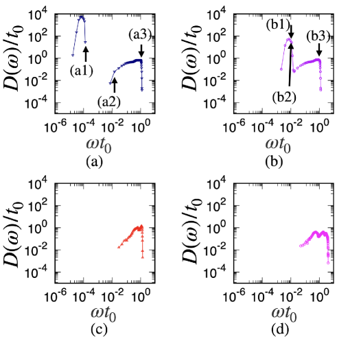
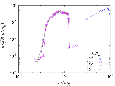
Because we have confirmed the existence of a peak of around , Fig. 10 shows the scaling of the DOS in Region I by plotting , where 333 The reason why is multiplied by in Fig. 10 is as follows. The integral value of the DOS within Region I is almost independent of . Then, LHS can be rewritten as a variable , where , and represents the integral in Region I. . From Fig. 10 we have confirmed that can be expressed as a universal scaling function of for and .
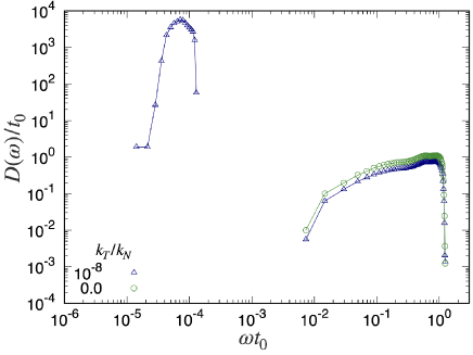
To clarify the behavior of the DOS in the frictionless limit, we compare the DOS for with that for frictionless particles by plotting both cases, where we adopt the Hessian matrix to calculate the DOS for frictionless systems (see Fig. 11 and Appendix H). As expected, there is no singularity of the DOS for the translational mode, while the isolated rotational band in low is absent in frictionless particles, as shown in Fig. 11.
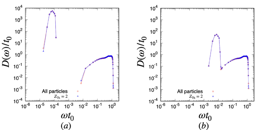
At the end of this subsection, we examine the usefulness of the effective Hessian introduced in Refs. Somfai07 ; Henkes10 ; Liu21 by comparing with , where is the DOS obtained from (see Appendix H). As shown in Figs. 12 (a) and (b), and for various are almost identical. Here, the peak of the DOS near is caused by the rotational motion of the grains. This agreement between the Jacobian and Hessian analyses is natural because the configuration before the application of shear was prepared with frictionless particles, and the tangential displacement is sufficiently small.
V Concluding Remarks
We analyzed the eigenmodes of the Jacobian and obtained an expression for the rigidity of amorphous solids of frictional particles under an infinitesimal strain. We reproduced the rigidity in the linear response regime using the eigenvalues and eigenfunctions of the Jacobian with modifications in the rotational part.
Further, we confirmed that the DOS can be divided into two regions for small . In the low-frequency region (Region I), the rotation of the particles plays a dominant role. These modes are characterized by the frequency . Region I merges into the high-frequency region (Region II) for large , where Region II is dominated by translational modes.
It should be noted that our results are almost independent of system size, as shown in Appendix I. Moreover, we have briefly analyzed the density dependence of the DOS in Appendix J, where the rotational band shifts to a lower frequency region and the plateau of the translational band become longer as the density approaches the jamming point.
We have also confirmed that the results of our Jacobian analysis are almost equivalent to those of the Hessian matrix. This is because our preparation of the initial configuration of grains is made by frictionless grains. Nevertheless, we expect that the Hessian analysis might be sufficient for stable configurations of grains.
However, the applicability of this theory is limited. The method used in this study cannot be used for finite strains because it is obvious that the eigenvectors are not orthogonal in the sheared state. Moreover, there are plastic deformations of the grains under large strains, which were not considered in this study. Therefore, we cannot predict the correct value of the theoretical rigidity at the stress drop point. More importantly, the effect of the history dependence of the frictional force is significant even in the linear response regime, although we have ignored such contacts because of the difficulty in constructing a proper theory. This issue should be addressed in future studies Ishima22 .
VI ACKNOWLEDGMENTS
The authors thank N. Oyama and T. Kawasaki for fruitful discussions and useful comments. This work was partially supported by a Grant-in-Aid from the MEXT for Scientific Research (Grant No. JP22K03459, JP21H01006, and JP19K03670) and by the Grant-in-Aid from the Japan Society for Promotion of Science JSPS Research Fellow (Grant No. JP20J20292).
Appendix A Method of preparing configuration before applying the shear
In this Appendix, we summarize the method of preparing a stable configuration of grains before applying the shear. For this purpose, as the first step, we perform the relaxation for frictionless particles with the FIRE. As the second step, the system is relaxed taking into account the static friction between particles. In the first subsection, we summarize how to prepare the configurations of frictionless particles by the FIRE Bitzek06 . In the second subsection, we describe the details of the numerical method including the force with static friction.
A.1 Method of preparing configuration before applying shear by FIRE
At first, we place particles at random without any overlaps of particles with the initial fraction . We increase the projected area fraction of the system by the increment of the fraction up to the target fraction , where and are the projected area fraction of the system before and after each step of the increment, respectively. After each step of the increment, the system is relaxed by the FIRE Bitzek06 .
To implement the process of increasing the area fraction, we scale the system as
| (1) | ||||
| (2) |
where and are the linear system size and the position of the -th particle before/after rescaling, respectively. We adopt . When there are overlaps between particles at , the system relaxes to a stable configuration with the aid of the FIRE.
The FIRE is a fast relaxation method of minimizing potentials depending on the configuration of the particles with Bitzek06 . Here, we use the Hertzian potential for which is defined as
| (3) |
Let us introduce -component of the force acting on the -th particle as
| (4) |
where or . Note that only consists of the normal repulsive force. In the FIRE the position and velocity with are updated by the following rules from (i) to (iv) with the variable time increment . (i) The numerical integration via the velocity Verlet method is performed on and :
| (5) | ||||
| (6) |
where is the updated configuration in Eq. (5). (ii) We calculate , where with . (iii) The velocity is updated as
| (7) |
where is the relaxation parameter and for an arbitrary vector . (iv) We update and in the FIRE according to the positive or negative value of . To speed up the relaxation when the motion is along a potential gradient, we increase . Note that this process is performed only when the number of numerical integrations along the potential gradient is larger than a certain number of times to stabilize the numerical calculation. To implement this update rule, if and the number of numerical integrations of is larger than , and are updated as
| (8) | ||||
| (9) |
where is a selecting function of smaller one from and , the parameter is introduced to speed up the relaxation, and , and are parameters to stabilize numerical calculations. Here, we adopt , and Bitzek06 ; Saitoh19 . Note that is necessary for the stability of the algorithm. In the case of , we set
| (10) | ||||
| (11) | ||||
| (12) |
We repeat the operations (i) through (iv) until for arbitrary and . Note that we have used the initial values for and at the starting point of the FIRE. Here, is given and we set at the starting point of the FIRE.
A.2 Numerical method for relaxation of configuration of frictional particles
After we obtain a stable configuration of frictionless particles at a target fraction in terms of the FIRE, we consider the effect of static friction in the relaxation process of frictional particles. The time evolution of the system is given by Eqs. (1)-(8) until for arbitrary and . For the time integration, we adopt the velocity Verlet method with the time increment .
Appendix B Velocity Verlet method in our system
In this Appendix, we first verify the accuracy of the velocity Verlet method. Next, we summarize the implementation of the velocity Verlet method. To simplify the notation, we introduce the generalized force with in this Appendix, where is for and for . Note that is the generalized force which depends on and as in Eqs. (3)-(8), where for an arbitrary vector .
B.1 Accuracy of the velocity Verlet method for the force depending on the velocity
In this subsection, we check the accuracy of the velocity Verlet method for the force depending on the velocity with the aid of discretization based on the Taylor expansion. The velocity Verlte method is given by a set of equations
| (13) | ||||
| (14) |
The first equation is called the velocity Velret equation for and the second one is the equation for . It is known that the velocity Verlet algorithm has the accuracy of in Hamiltonian systems Swope82 , but the accuracy of this method for dissipative dynamics is little known. Therefore, we clarify the accuracy of this method in this Appendix.
Here, we show from the Taylor expansion that the velocity Verlet method has a second-order and first-order accuracies of for and , respectively. Based on the Taylor expansion of , we obtain
| (15) |
where for an arbitrary function . We can obtain the quadratic precision of for , because the RHS of Eq. (15) is a function of current time .
On the other hand, based on the Taylor expansion of , we obtain
| (16) |
By using , we evaluate as
| (17) |
Substituting Eq. (17) into Eq. (16), we obtain Swope82
| (18) |
If the force is independent of , we can obtain from with the aid of Eq. (15) Swope82 . However, if depends on , we have to evaluate , because requires LHS of Eq. (18). Thus, we adopt the following replacements:
| (19) | ||||
| (20) |
where we have introduced
| (21) | ||||
| (22) |
Here, the difference between and caused by Eq. (19) is given by
| (23) |
Similarly, the difference between and in Eq. (20) can be evaluated as
| (24) |
Thus, the replacement of Eqs. (19) and (20) in Eq. (18) with Eqs. (23) and (24) leads to
| (25) |
Omitting the term including in Eq.(25), we obtain the following numerical integration methods for :
| (26) |
Note that Eq. (26) is the precise expression of the velocity Verlet scheme for presented in Eq. (14). From the comparison between Eqs. (25) and (26), we have confirmed that the velocity Verlet scheme has the first-order precision of for . We also note that if is independent of as in the case of Hamiltonian systems, the term proportional to is zero and thus, the second-order accuracy of for is guaranteed.
Let us go back to Eq. (15) with the replacement of Eq. (20) for :
| (27) |
Omitting the term including in Eq.(27), we obtain the following numerical integration methods for :
| (28) |
Here, Eq. (28) is the precise expression of the velocity Verlet scheme for presented in Eq. (13). From Eqs. (27) and (28) we have confirmed that the velocity Verlet scheme has the second-order precision of for .
B.2 Implementation of the velocity Verlet method for the force depending on the velocity
In this subsection, we explain how to adopt the velocity Verlet method in our system. In the main text, we adopt the following equations:
| (29) | ||||
| (30) |
Here, the updated configuration and modified velocity are used to obtain the force . Then, we update the velocity as follows
| (31) |
Appendix C Jacobian Properties
In this Appendix, we summarize the properties of the Jacobian introduced in Eq. (18).
C.1 Jacobian block elements
Let us write sub-matrix , which is block element of the Jacobian obtained from Eq. (18):
| (32) |
where the superscripts and correspond to -components, and and are the particle numbers (see Appendix F for each component of ). Here, are -component of and scaled torque that the -th particle receives from the -th particle, respectively. The sub-matrix for is given by
| (33) |
where we have used , and . Here, the superscripts and correspond to components.
From Eqs. (32) and (33) satisfies
| (34) |
Thus, introducing which is a rewriting of in Eq. (19) by the index from and to , we obtain
| (35) | ||||
| (36) |
where and express the summations of modulus and modulus with the intervals , respectively. Here, we write -dimensional vector translating in the direction as
| (37) |
where for . Here, the -th component of the action of on satisfies
| (38) |
where we have used Eq. (35) for the last equality. Thus, we obtain , where is zero vector. Similarly, using
| (39) |
with we also obtain . Therefore, and are the zero modes for .
Appendix D Explicit Jacobian expressions
In this Appendix, we present the explicit expressions of the Jacobian based on Eqs. (6)-(8). Then, we clarify the difference between the present results and the case where the tangential force is approximated by the conservative force used in the previous studies Somfai07 ; Henkes10 .
D.1 Calculation of Jacobian
Let us consider only the normal and tangential elastic contact forces
| (40) | ||||
| (41) |
where the integration of
| (42) |
is performed during the contact between and particles. Since Eq. (42) does not contain the second term on RHS of Eq. (9), may not be perpendicular to . Neverthelss, we adopt Eq. (42) for simplicity. Here, is defined as
| (43) |
where is defined as
| (44) |
Each component of Eq. (43) is written as
| (45) | ||||
| (46) |
The derivative of the normal force is given by
| (47) | ||||
| (48) |
where Kronecker’s delta satisfies for and otherwise. We have used
| (49) | ||||
| (50) |
to obtain Eq. (47).
The derivative of the tangential force is written as
| (51) | ||||
| (52) |
where and are, respectively, defined as
| (53) | ||||
| (54) |
Here, and in Eqs. (51) and (52) satisfy
| (55) | ||||
| (56) |
The derivation of Eqs. (55) and (56) are as follows Chattoraj19 . From Eq. (43) can be written as
| (57) |
Then, satisfies
| (58) |
Similarly, also satisfies
| (59) |
Here, is the function of and . We obtain the differential form of :
| (60) |
Then, we obtain Eqs. (55), (56), by comparing Eqs. (58) and (59) with Eq. (60).
Since the scaled torque satisfies
| (61) |
we obtain
| (62) | ||||
| (63) |
where we have used .
The terms proportional to in the Jacobian include the history-dependent tangential displacements which are ignored in the effective potential (see Appendix H) Somfai07 ; Henkes10 ; Liu21 . The reason we use the Jacobian is to include the history-dependent tangential displacements in the dynamical matrix.
Appendix E Effects of rattlers
In this Appendix, we investigate the effects of rattlers. In the first subsection, we investigate the effects of rattlers for the DOS. In the second subsection, we clarify the contributions of rattlers by using the participation ratio.
E.1 Effects of rattlers on the DOS
In this subsection, we investigate the role of rattlers. We call particle a rattler, if its coordination number is . Since the coordination number of isostatic state is three, can be or for frictional grains. The rattlers are determined by the following method. Given a particle configuration, we measure the coordination number of each particle. Then, we regard particles satisfying as rattlers at the first trial. We measure the coordination number after we remove the rattler particles. In the second trial, we regard particles satisfying as new rattlers. We repeat these processes until the number of rattlers is converged. As shown in Fig. 13, at which we adopt , low-frequency modes in Region I and intermediate modes between Regions I and II are contributions from rattlers. Thus, we conclude that the contributions of rattlers on the DOS are not important.
E.2 Participation ratio
In this subsection, to clarify whether the mode at is localized or spread to the whole system, we introduce a participation ratio Yunker11 ; Shiraishi19
| (64) |
We plot defined as
| (65) |
against for in Fig. 14. Note that are set to be zero if there is no right eigenvalue in the region .
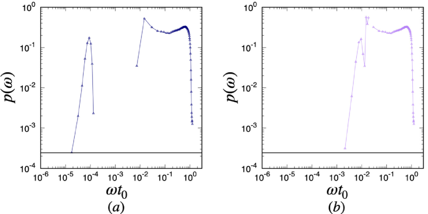
Figure 14 shows that the modes at in Fig. 14 (a) and at in Fig. 14 (b) are nearly equal to . Recalling that those modes consist of the rattler, we conclude that the contribution of the rattler is localized. In the middle range of in Fig. 14, there is an isolated band which shifts to the large as increases with keeping its shape which can be seen in the main text.
Appendix F Explicit results of and
In this Appendix, we have written down the explicit results of and . From the results for the derivative of in Appendix D , the non-diagonal block elements are given by
| (66) | ||||
| (67) | ||||
| (68) | ||||
| (69) | ||||
| (70) | ||||
| (71) | ||||
| (72) | ||||
| (73) | ||||
| (74) | ||||
| (75) | ||||
| (76) | ||||
| (77) | ||||
| (78) | ||||
| (79) | ||||
| (80) | ||||
| (81) | ||||
| (82) | ||||
| (83) |
Similarly, the diagonal block elements are given by
| (84) | ||||
| (85) | ||||
| (86) | ||||
| (87) | ||||
| (88) | ||||
| (89) | ||||
| (90) | ||||
| (91) | ||||
| (92) | ||||
| (93) | ||||
| (94) | ||||
| (95) | ||||
| (96) | ||||
| (97) | ||||
| (98) | ||||
| (99) | ||||
| (100) | ||||
| (101) |
Note that the terms proportional to in include the history-dependent tangential displacements which are ignored in the effective potential Somfai07 ; Henkes10 ; Liu21 .
Appendix G The detailed derivation of in the Jacobian analysis
In this Appendix, we derive Eq. (38) that gives the rigidity. First, nonaffine displacements are expanded in terms of eigenfunctions of the Jacobian. Next, we express the rigidity as the eigenvalues and eigenfunctions of the Jacobian. Note that we adopt the abbreviation in this Appendix.
G.1 Expansion for nonaffine displacements via eigenfunction of Jacobian
At FB state, is expressed as
| (102) |
Using the Jacobian, we rewrite Eq. (102) as
| (103) |
where the first and second terms on the RHS represent the contributions from the affine and nonaffine displacements, respectively. Since the affine displacements are applied to our system instantaneously as a step strain, the integral interval of tangential displacements during the affine deformation are zero. Thus, only the normal contributions in the first term on RHS of Eq. (103) survive in the affine displacements. Then, we rewrite as in Eq. (103):
| (104) |
Since satisfies , we obtain
| (107) |
Since satisfies , we obtain
| (108) |
Let us introduce as
| (109) |
and
| (110) |
Here, satisfies
| (111) |
With the aid of Eqs. (107) and (108) are rewritten as
| (112) | ||||
| (113) |
Equations (112) and (113) can be rewritten as
| (114) |
Furthermore, Eq. (114) can be expressed as
| (115) |
which corresponds to Eq. (34) in the main text, where is introduced in Eq. (33).
G.2 The expression of
Let us evaluate the rigidity defined as Eq. (17). Substituting Eqs. (14) and (15) into Eq. (17), we obtain
| (119) |
where we have adopted the symmetric expression for and in the summation in Eq. (119).
Expanding in Eq. (119) by from the zero strain state, we obtain
| (120) |
Similarly, expanding in Eq. (119) from the zero strain state, we obtain
| (121) |
Furthermore, using and , can be written as
| (122) |
Appendix H DOS in terms of the effective Hessian
In this Appendix, we introduce the DOS with the aid of the effective Hessian as in Refs. Somfai07 ; Henkes10 ; Liu21 . The effective Hessian at the FB state is defined as
| (127) |
where is the effective potential defined as
| (128) |
with , and . Here, and are the position of -th particle and rd component of at the FB state, respectively. Thus, is a matrix corresponding to the Jacobian. We note that this Hessian matrix is a real symmetric matrix, and thus, it can be diagonalized by an orthogonal matrix, where the eigenvectors are orthogonal with each other, and the corresponding eigenvalues are real number.
The eigenvalue equation of is expressed as
| (129) |
where and are the -th eigenvalue and eigenvector of , respectively. Note that the left eigenvalue is also given by , where . Then, we introduce the DOS in terms of as
| (130) |
where .
Appendix I System size dependence for the DOS
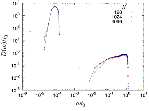
The system size dependence of the DOS is investigated in this Appendix. From Fig. 15 we have confirmed that both the rotational and translational bands show little dependence on system size. This means that the rotational band is not a virtual band that can only be observed in a small system, but an intrinsic band that can be observed in the thermodynamic limit. Thus, we expect that our observed results will remain unchanged even if we are interested in larger systems.
Appendix J Density dependence for DOS
In this Appendix, we investigate the density dependence for the DOS. As shown in Fig. 16 for , the DOS depends on , where the rotational band shifts to a lower frequency region and the plateau of the translational band becomes longer as the density approaches the jamming point. The latter result is well known from previous studies such as Ref. Wyart05 .
References
- (1) H. M. Jaeger, S. R. Nagel, and R. P. Behringer, Granular solids, liquids, and gases, Rev. Mod. Phys. 68, 1259 (1996).
- (2) D. J. Durian, Foam Mechanics at the Bubble Scale, Phys. Rev. Lett. 75, 4780 (1995).
- (3) M. Wyart, On the rigidity of amorphous solids, Ann. Phys. Fr. 30, 1 (2005).
- (4) A. Baule, F. Morone, H. J. Herrmann, and H. A. Makse, Edwards statistical mechanics for jammed granular matter, Rev. Mod. Phys. 90, 015006 (2018).
- (5) A. Liu and S. Nagel, Jamming is not just cool any more, Nature (London) 396, 21 (1998).
- (6) C. S. O’Hern, L. E. Silbert, A. J. Liu, and S. R. Nagel, Jamming at zero temperature and zero applied stress: The epitome of disorder, Phys. Rev. E 68, 011306 (2003).
- (7) C. S. O’Hern, S. A. Langer, A. J. Liu, and S. R. Nagel, Force Distributions near Jamming and Glass Transitions, Phys. Rev. Lett. 86, 111 (2001).
- (8) V. Trappe, V. Prasad, L. Cipelletti, P. N. Segre, and D. A. Weitz, Jamming phase diagram for attractive particles, Nature (London) 411, 772 (2001).
- (9) H. P. Zhang and H. A. Makse, Jamming transition in emulsions and granular materials, Phys. Rev. E 72, 011301 (2005).
- (10) T. S. Majmudar, M. Sperl, S. Luding, and R. P. Behringer, Jamming Transition in Granular Systems, Phys. Rev. Lett. 98, 058001 (2007).
- (11) M. P. Ciamarra, R. Pastore, M. Nicodemi, and A. Coniglio, Jamming phase diagram for frictional particles, Phys. Rev. E 84, 041308 (2011).
- (12) K. Hima Nagamanasa, S. Gokhale, A. K. Sood, and R. Ganapathy, Experimental signatures of a nonequilibrium phase transition governing the yielding of a soft glass, Phys. Rev. E 89, 062308 (2014).
- (13) E. D. Knowlton, D. J. Pine, and L. Cipelletti, A microscopic view of the yielding transition in concentrated emulsions, Soft Matter 10, 6931 (2014).
- (14) T. Kawasaki and L. Berthier, Macroscopic yielding in jammed solids is accompanied by a nonequilibrium first-order transition in particle trajectories, Phys. Rev. E 94, 022615 (2016).
- (15) P. Leishangthem, A. D.S. Parmar, and S. Sastry, The yielding transition in amorphous solids under oscillatory shear deformation, Nat. Commun. 8, 14653 (2017).
- (16) S. Dagois-Bohy, E. Somfai, B. P. Tighe, and M. van Hecke, Softening and yielding of soft glassy materials , Soft Matter 13, 9036 (2017).
- (17) M. Ozawa, L. Berthier, G. Biroli, A. Rosso, and G. Tarjus, Random critical point separates brittle and ductile yielding transitions in amorphous materials, Proc. Natl.Acad. Sci. U.S.A. 115, 6656 (2018).
- (18) A. H. Clark, J. D. Thompson, M. D. Shattuck, N. T. Ouellette, and C. S. O’Hern, Critical scaling near the yielding transition in granular media, Phys. Rev. E 97, 062901 (2018).
- (19) J. Boschan, S. Luding, and B. P. Tighe, Jamming and irreversibility, Granul. Matter 21, 58 (2019).
- (20) M. Singh,M. Ozawa, and L. Berthier, Brittle yielding of amorphous solids at finite shear rates, Phys. Rev. Materials 4, 025603 (2020).
- (21) M. Otsuki and H. Hayakawa, Softening and residual loss modulus of jammed grains under oscillatory shear in absorbing state, Phys. Rev. Lett. 128, 208002 (2022).
- (22) M. Wyart, S. R. Nagel, and T. A. Witten, Geometric origin of excess low-frequency vibrational modes in weakly connected amorphous solids, Eur. Phys. Lett. 72, 486 (2005).
- (23) W. G. Ellenbroek, E. Somfai, M. van Hecke, and W. van Saarloos, Critical Scaling in Linear Response of Frictionless Granular Packings near Jamming, Phys. Rev. Lett. 97, 258001 (2006).
- (24) E. Lerner, G. Düring, and E. Bouchbinder, Statistics and Properties of Low-Frequency Vibrational Modes in Structural Glasses, Phys. Rev. Lett. 117, 035501 (2016).
- (25) L. Gartner and E. Lerner, Nonlinear plastic modes in disordered solids, Phys. Rev. E 93, 011001(R) (2016).
- (26) S. Bonfanti, R. Guerra, C. Mondal, I. Procaccia, and S. Zapperi, Elementary plastic events in amorphous silica, Phys. Rev. E 100 060602(R) (2019).
- (27) E. DeGiuli, E. Lerner, C. Brito, and M. Wyart, Force distribution affects vibrational properties in hard-sphere glasses, Proc. Natl.Acad. Sci. U.S.A. 111, 17054 (2014).
- (28) H. Mizuno, K. Saitoh, and L. Silbert, Elastic moduli and vibrational modes in jammed particulate packings, Phys. Rev. E 93, 062905 (2016).
- (29) C. Maloney and A. Lemaître, Universal Breakdown of Elasticity at the Onset of Material Failure, Phys. Rev. Lett. 93, 195501 (2004).
- (30) C. Maloney and A. Lemaître, Amorphous systems in athermal, quasistatic shear, Phys. Rev. E 74, 016118 (2006).
- (31) A. Lemaître and C. Maloney, Sum Rules for the Quasi-Static and Visco-Elastic Response of Disordered Solids at Zero Temperature, J. Stat. Phys. 123, 415 (2006).
- (32) A. Zaccone and E. Scossa-Romano, Approximate analytical description of the nonaffine response of amorphous solids, Phys. Rev. B 83, 184205 (2011).
- (33) M. L. Manning and A. J. Liu, Vibrational Modes Identify Soft Spots in a Sheared Disordered Packing, Phys. Rev. Lett. 107, 108302 (2011).
- (34) R. Dasgupta, S. Karmakar, and I. Procaccia, Universality of the Plastic Instability in Strained Amorphous Solids, Phys. Rev. Lett. 108, 075701 (2012).
- (35) F. Ebrahem, F. Bamer, and B. Markert, Origin of reversible and irreversible atomic-scale rearrangements in a model two-dimensional network glass, Phys. Rev. E 102, 033006 (2020).
- (36) R. C. Zeller and R. O. Pohl, Thermal Conductivity and Specific Heat of Noncrystalline Solids, Phys. Rev. B 4, 2029 (1971).
- (37) A. Nicolas, E. E. Ferrero, K. Martens, and J.-L. Barrat, Deformation and flow of amorphous solids: Insights from elastoplastic models, Rev. Mod. Phys., 90, 045006 (2018).
- (38) W. Schirmacher, G. Ruocco, and T. Scopigno, Acoustic Attenuation in Glasses and its Relation with the Boson Peak, Phys. Rev. Lett., 98, 025501 (2007).
- (39) H. Mizuno, H. Shiba, and A. Ikeda, Continuum limit of the vibrational properties of amorphous solids, Proc. Natl.Acad. Sci. U.S.A. 114, 9767 (2017).
- (40) L. Wang, A. Ninarello, P. Guan, L Berthier, G. Szamel, and E. Flenner, Low-frequency vibrational modes of stable glasses, Nat. Commun. 10, 26 (2019).
- (41) Z. Zeravcic, N. Xu, A. J. Liu, S. R. Nagel, and W. van Saarloos, Excitations of ellipsoid packings near jamming, Eur. Phys. Lett. 87, 26001 (2009).
- (42) M. Mailman, C. F. Schreck, C. S. O’Hern, and B. Chakraborty, Jamming in Systems Composed of Frictionless Ellipse-Shaped Particles, Phys. Rev. Lett. 102, 255501 (2009).
- (43) C. F. Schreck, N. Xu, and C. S. O’Hern, A comparison of jamming behavior in systems composed of dimer- and ellipse-shaped particles, Soft Matter 6, 2960 (2010).
- (44) P. J. Yunker, K. Chen, Z. Zhang, W. G. Ellenbroek, A. J. Liu, and A. G. Yodh, Rotational and translational phonon modes in glasses composed of ellipsoidal particles, Phys. Rev. E 83, 011403 (2011).
- (45) C. F. Schreck, M. Mailman, B. Chakraborty,and C. S. O’Hern, Constraints and vibrations in static packings of ellipsoidal particles, Phys. Rev. E 85, 061305 (2012).
- (46) K. Shiraishi, H. Mizuno, and A. Ikeda, Vibrational properties of two-dimensional dimer packings near the jamming transition, Phys. Rev. E 100, 012606 (2019).
- (47) S. Papanikolaou, C. S. O’Hern, and M. D. Shattuck, Isostaticity at Frictional Jamming, Phys. Rev. Lett. 110, 198002 (2013).
- (48) C. Brito, H. Ikeda, P. Urbanic, M. Wyartd, and F. Zamponi, Universality of jamming of nonspherical particles, Proc. Natl.Acad. Sci. U.S.A. 115, 11736 (2018).
- (49) J. D. Treado, D. Wang, A. Boromand, M. P. Murrell, Mark D. Shattuck, and C. S. O’Hern, Bridging particle deformability and collective response in soft solids, Phys. Rev. Matt. 5, 055605 (2021).
- (50) H. Ikeda, C. Brito, M. Wyart, and F. Zamponi, Jamming with Tunable Roughness, Phys. Rev. Lett. 124, 208001 (2020).
- (51) H. Ikeda, Testing mean-field theory for jamming of non-spherical particles: contact number, gap distribution, and vibrational density of states, Eur. Phys. E 44, 120 (2021).
- (52) E. Somfai, M. van Hecke, W. G. Ellenbroek, K. Shundyak, and W. van Saarloos, Critical and noncritical jamming of frictional grains, Phys. Rev. E 75, 020301(R) (2007).
- (53) S. Henkes, M. van Hecke, and W. van Saarloos, Critical jamming of frictional grains in the generalized isostaticity picture, Eur. Phys. Lett. 90, 14003 (2010).
- (54) K. Liu , J. E. Kollmer , K. E. Daniels, J. M. Schwarz, and S. Henkes, Spongelike Rigid Structures in Frictional Granular Packings, Phys. Rev. Lett. 126, 088002 (2021).
- (55) J. Chattoraj, O. Gendelman, M. Pica Ciamarra, and I. Procaccia, Oscillatory Instabilities in Frictional Granular Matter, Phys. Rev. Lett. 123, 098003 (2019).
- (56) J. Chattoraj, O. Gendelman, M. P. Ciamarra, and I. Procaccia, Noise amplification in frictional systems: Oscillatory instabilities, Phys. Rev. E 100, 042901 (2019).
- (57) H. Charan,O. Gendelman, I. Procaccia, and Y. Sheffer, Giant amplification of small perturbations in frictional amorphous solids, Phys. Rev. E 101, 062902 (2020).
- (58) S. Luding, Global equation of state of two-dimensional hard sphere systems, Phys. Rev. E 63, 042201 (2001).
- (59) G. Kuwabara and K. Kono, Restitution Coefficient in a Collision between Two Spheres, Jpn. J. Appl. Phys. 26, 1230 (1987).
- (60) N. V. Brilliantov, F. Spahn, J.-M. Hertzsch, and T. Pöschel, Model for collisions in granular gases, Phys. Rev. E 53, 5382 (1996).
- (61) W. A. M. Morgado and I. Oppenheim, Energy dissipation for quasielastic granular particle collisions, Phys. Rev. E 55, 1940 (1997).
- (62) M. Otsuki and H. Hayakawa, Discontinuous change of shear modulus for frictional jammed granular materials, Phys. Rev. E 95, 062902 (2017).
- (63) E. Bitzek, P. Koskinen, F. Gähler, M. Moseler, P. Gumbsch, Structural Relaxation Made Simple, Phys. Lev. Lett. 97, 170201 (2006).
- (64) A. Lees and S. Edwards, The computer study of transport processes under extreme conditions, J. Phys. C: Solid State Phys. 5, 1921 (1972).
- (65) D. J. Evans and G. P. Morriss, Statistical Mechanics of Nonequilibrium Liquids, 2nd ed. (Cambridge University Press, Cambridge, UK, 2008).
- (66) P. Olsson and S. Teitel, Critical scaling of shearing rheology at the jamming transition of soft-core frictionless disks, Phys. Rev. E 83, 030302(R) (2011).
- (67) M. Otsuki and H. Hayakawa, Critical scaling near jamming transition for frictional granular particles, Phys. Rev. E 83, 051301 (2011).
- (68) D. Ishima and H. Hayakawa, Scaling laws for frictional granular materials confined by constant pressure under oscillatory shear, Phys. Rev. E 101, 042902 (2020).
- (69) W. C. Swope, H. C. Andersen, P. H. Berens, and K. R. Wilson, A computer simulation method for the calculation of equilibrium constants for the formation of physical clusters of molecules: Application to small water clusters, J. Chem. Phys. 76, 637 (1982).
- (70) K. Saitoh, R. Shrivastava, and S. Luding, Rotational sound in disordered granular materials, Phys. Rev. E 99, 012906 (2019).
- (71) D. Ishima, K. Saitoh, M. Otsuki and H. Hayakawa, Eigenvalue analysis of stress-strain curve of two-dimensional amorphous solids of dispersed frictional grains with finite shear strain, arXiv.2212.04628 (to be published in Phys. Rev. E).