,
Theory of polarization-averaged core-level molecular-frame photoelectron angular distributions: III. New formula for - and -wave interference analogous to Young’s double-slit experiment for core-level photoemission from hetero-diatomic molecules
Abstract
We present a new variation of Young’s double-slit formula for polarization-averaged molecular-frame photoelectron angular distributions (PA-MFPADs) of hetero-diatomic molecules, which may be used to extract the bond length. So far, empirical analysis of the PA-MFPADs has often been carried out employing Young’s formula in which each of the two atomic centers emits an -photoelectron wave. The PA-MFPADs, on the other hand, can consist of an interference between the -wave from the X-ray absorbing atom emitted along the molecular axis and the -wave scattered by neighboring atom, within the framework of Multiple Scattering theory. The difference of this - wave interference from the commonly used - wave interference causes a dramatic change in the interference pattern, especially near the angles perpendicular to the molecular axis. This change involves an additional fringe, urging us to caution when using the conventional Young’s formula for retrieving the bond length. We have derived a new formula analogous to Young’s formula but for the - wave interference. The bond lengths retrieved from the PA-MFPADs via the new formula reproduce the original C-O bond lengths used in the reference ab-initio PA-MFPADs within the relative error of 5 %. In the high energy regime, this new formula for - wave interference converges to the ordinary Young’s formula for the - wave interference. We expect it to be used to retrieve the bond length for time-resolved PA-MFPADs instead of the conventional Young’s formula.
Keywords: PA-MFPAD, MFPAD, PED, Multiple Scattering theory, Young’s formula, XFEL
1 Introduction
Tracking the real molecular dynamics is one of the main interests in chemistry, biology and physics. It provides us with deep insights into the properties of molecules, e.g., chemical reactions [1, 2, 3]. The recent development of X-ray free electron lasers (XFELs) [4, 5, 6, 7, 8, 9, 10] has enabled us to investigate the structural changes of molecules and solids in ultra-short-time resolution of the order of femtoseconds, due to their high brightness and short pulse width [11, 12, 13].
Core-level excitation X-ray spectroscopies such as X-ray absorption (XAS) and photoelectron diffraction (PED) are effective approaches for investigating the structure of non-periodic gases, liquids and amorphous systems since they do not require any periodicity. Extended X-ray absorption fine structure (EXAFS), a variant of XAS, and PED are conceptually similar: EXAFS scans the amplitude of the photoelectron momentum while PED is mostly used for scans of the direction of the photoelectron momentum and both provide information on the local structure around the core orbital where the X-ray absorption takes place [14]. PED is commonly used for surface structure analysis [15].
In order to apply PED to gas-phase molecules, the PED scan should be performed in the molecular frame. This is experimentally achieved by angle-resolved coincidence measurements between the core-level photoelectrons and the fragment ions [16]. The COLTRIMS-Reaction microscope [17] is a standard technique for studying molecular photoionization in the coincidence manner [18]: The COLTRIMS technique provides the angular distribution of photoelectrons in the molecular frame (Molecular-Frame Photoelectron Angular Distributions: MFPADs), which is equivalent to PED in gas phase molecules, by measuring simultaneously the momentum correlations between the core-level photoelectrons and the fragment ions.
Synchrotron radiation based studies [19, 20] have shown that MFPADs averaged over the polarization angle of incident X-rays (Polarization-Averaged Molecular-Frame Photoelectron Angular Distributions: PA-MFPADs) provide information on the structure of molecules. The beauty of polarization averaging is that the most prominent peaks produced by directly excited photoelectron waves, where the angular distribution of dipoles is parallel to the polarization vector, are smeared out, and the effect of scattering by surrounding atoms of the absorbing atoms is emphasized. Hence, PA-MFPADs reflect the three-dimensional structure information more clearly than MFPADs.
Several attempts aiming at tracing molecular dissociation through time-resolved MFPADs measurements have already been performed [21, 22, 23, 24] but without much success. This situation is dramatically changing now thanks to the emergence of the European XFEL, the first high repetition-rate XFEL [9], and of the COLTRIMS-Reaction microscope installed there [25]. Using sequential ionization of the O core level in the O2 molecule within a single XFEL pulse, it was demonstrated that time-resolved PA-MFPADs measurements are possible with XFEL [25]. Since an XFEL-pump–XFEL-probe system has also been installed there [26], making a molecular movie recording the PA-MFPADs is no longer an intangible dream but a tangible reality.
This article is the third in a series of articles on the theoretical study of PA-MFPADs for dissociating hetero-diatomic dications CO2+, which may be measured by pump-probe experiments with the two-color XFEL. In this type of experiment, the first XFEL pulse removes one of the core electrons and the subsequent Auger decay creates the CO2+ ion that starts to dissociate. Then one can probe the variations of the C-O bond length by the time-resolved PA-MFPADs measurement using the second XFEL pulse as a probe. In the first paper [27] in this series, we introduced the Full-potential Multiple Scattering (FPMS) theory and presented results for the calculation of PA-MFPADs of CO2+ as a function of the C-O bond length. In the second paper [28], we proposed a fitting method for the retrieval of the bond length from the EXAFS-type oscillations which appear in the backward scattering direction of the PA-MFPADs.
In this third paper, we derive an analytical formula that describes a fringe pattern of the PA-MFPAD, which may be identified as a flower shape. The formula derived can be used to estimate the bond length of dissociating hetero-diatomic molecules. Because this flower shape pattern is generated by the interference of two electron waves emitted respectively from the X-ray photon absorbing atom, and from the neighboring scattering atom, the mechanism that constitutes this flower shape may be interpreted as an analogue to Young’s double-slit experiment. However, the physical phenomena behind Young’s double-slit experiment and PA-MFPADs are not exactly the same. The key difference between them is that Young’s double-slit experiment represents the interference of two spherical -waves, while the O PA-MFPADs we are interested in consists in the interference between one -wave, which is the direct wave emitted by the atom that absorbs an X-ray photon, and the wave scattered by the neighboring atom, which may be approximated by an -wave. Using Multiple Scattering theory, we derive a new formula for the - wave interference in the PA-MFPADs, analogous to Young’s formula for the - wave interference, and further examine the validity of this new formula, by applying it to the PA-MFPADs of dissociating CO2+ calculated within the FPMS theory [27]. We also discuss the issue of applying the original Young’s formula to the analysis of PA-MFPADs.
2 Theory
In this section, we derive analytical expressions for the flower shape structure that appears as an oscillatory structure when varying the angles in the PA-MFPADs. We first give an expression to determine the angles of the bright and dark fringes of PA-MFPADs. Next, utilizing this result, we derive a relationship between the low and high angle fringes.
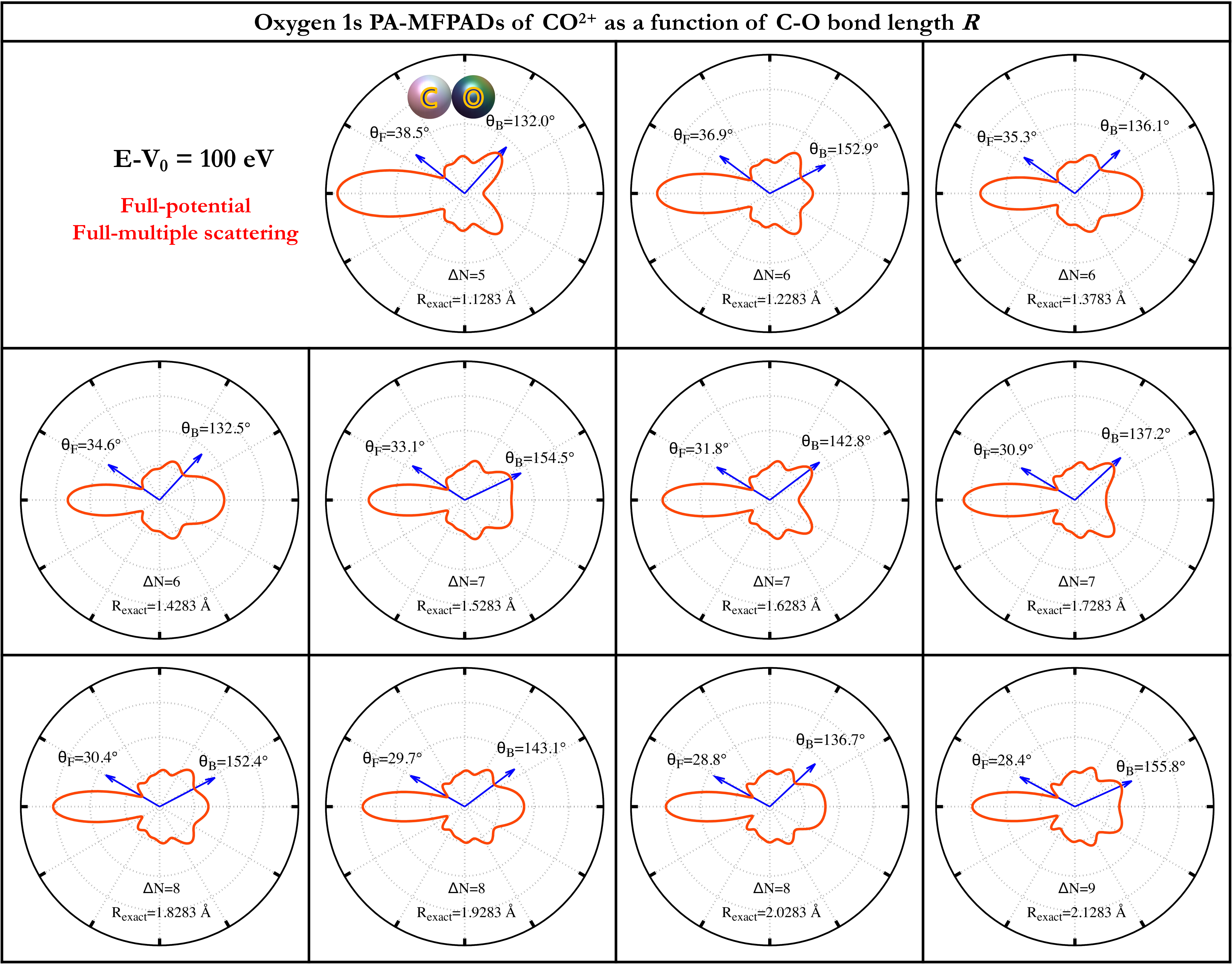
Figure 1 depicts PA-MFPADs calculated as a function of the C-O bond length , using the FPMS theory of PA-MFPADs for photoelectrons of momentum k [27]
| (1) | |||
| (2) |
where
| (3) |
and
| (4) | |||||
| (5) |
The indices and refer to the scattering sites and . is the fine structure constant, is the vector connecting the origin to the center of scattering site and is the real spherical harmonics of angular momentum . In the second line of equation 2, is the Gaunt coefficient composed of real spherical harmonics and the rest is the radial integral between the local solution and the core wave function. In equation 4, is the transition operator and is the KKR structure factor; They are matrices labeled with the indices referring to scattering sites and angular momentum [29, 30].
We see that the PA-MFPADs intensity which is defined as the average over polarization angle of MFPADs intensity is equivalent to the average over the three MFPADs with the polarization vector along the , and -axes respectively. More details are reported in the preceding paper [27] in this series. The electron charge density was calculated at the RASPT2/ANO-RCC-VQZP level of theory as implemented in MOLCAS 8.2 [31] for the multiplet state 15 (i.e. O 1 HOMO-2) considered as the dominant Auger final state [32]. We chose for the photoelectron energy eV. Several small lobes appear between the forward- and backward-intensity peaks. The elongation of the bond length moves these lobes from the backward to the forward position and increases their number by one for one period of oscillation of the backward-intensity peak.
From a simple physical insight, we identify the flower shape structure at the intermediate angles as a signature of the interference between the direct wave of the photoelectron originating from the oxygen atom and the photoelectron wave scattered by the carbon atom. This process strongly resembles a Young’s double-slit experiment. The following formula, the so-called Young’s formula, obtained from classical wave mechanics describes the relationship connecting the distance between the two slits to the two fringes angles and ,
| (6) |
where the positive integers and are index numbers identifying the and bright or dark fringes counted from the angle zero along the two slit axis. This formula is conventionally used to determine the bond length of molecules for PA-MFPADs. However, it is only valid for a two -wave interference. This is not the case of PA-MFPADs which originate from the interference between the -wave of the O 1 photoelectron ejected from the X-ray photon absorbing atom mostly through an electron dipole transition along the molecular axis, and the scattered wave from the neighbouring atom at distance , which may be approximated by an -wave.The purpose of this article is to derive a corresponding formula for this - interference within the framework of quantum scattering theory.
In order to obtain a relationship between and for PA-MFPADs, we start from the following formula for PA-MFPADs within the single-scattering plane wave and Muffin-tin approximations [28],
| (7) |
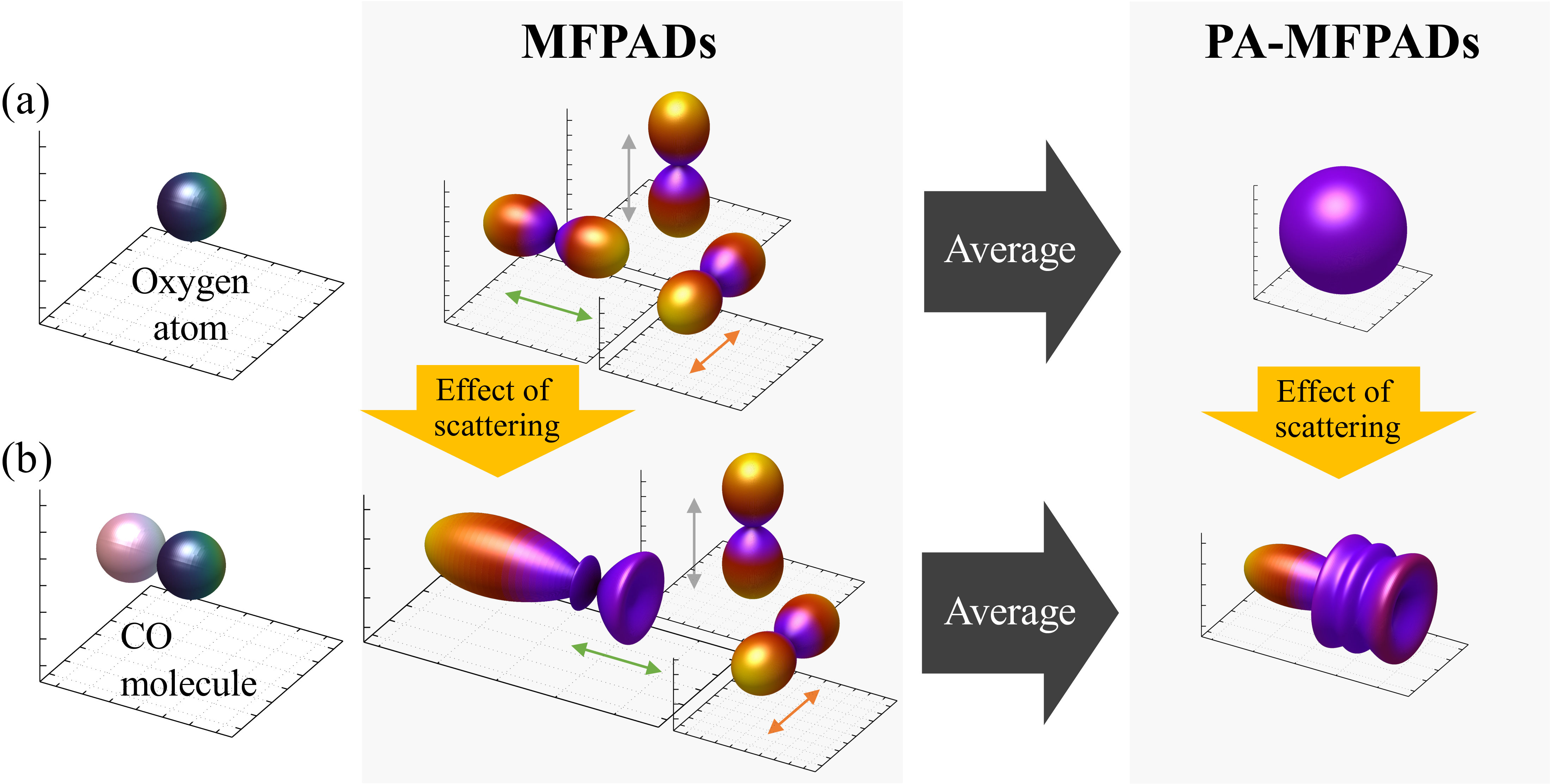
where is the scattering amplitude and the superscripts denote the scattering atom, i.e. for carbon and for oxygen. We remind that, as the CO2+ is arranged to have its molecular axis parallel to the -axis, and . Thus, the second and third terms in equation 7 are due only to the component . In this physical picture, only O photoelectrons excited by X-rays polarized parallel to the molecular axis propagate to the neighboring atom and are scattered, whereas the ones excited by X-rays with a polarization perpendicular to the molecular axis are not scattered, as explicited in the MFPADs in figure 2(b).
Performing the summation over , we obtain
| (8) |
The summation corresponds to the sum of the MFPADs excited by three orthogonal linearly polarized lights shown in the center of figure 2(b) and the result of equation 8 is the PA-MFPADs shown in the right hand side in figure 2(b). The first term corresponds to the direct photoemission process where no scattering occurs after emission by the photo-absorbing atom. This term corresponds to the atomic PA-MFPADs in figure 2(a), and indeed it does not depend on the angles. The third term corresponds to the intensity of a wave singly scattered by the neighboring carbon atom, and the second term corresponds to the interference between the direct wave and the singly scattered wave. This second term gives rise to the fringes observed at intermediate angles, which can be identified to the wrinkles in the PA-MFPADs in figure 2(b), and which we refer to as a ”flower shape” pattern.
We define now the following function which is responsible for the flower shape in the second term in equation 8,
| (9) |
where is the phase function of the scattering amplitude, . The modulus function is a smooth function of the angle when compared to the rest in the second term in equation 8, so that we can neglect the dependence in for the study of the flower shape. We hereafter omit the argument since we focus on PA-MFPADs at a given energy. The zeros in the derivative of this function with respect to correspond to the positions of fringes. Thus, the equation to be solved is
The zeros at and from the are of no interest to us since there, we can not distinguish the contribution to the interferences from that of the large forward- and backward-intensities. We therefore look for the zeros inside the brackets and the equation to be solved becomes
where is an integer. This equation can not be solved exactly and therefore we introduce some simplifications in order to obtain approximate solutions.
Here, we assume that . In order to make the integer correspond to the numbering of the fringe, the LHS of equation 2 needs to be a function that increases as increases from 0 to . On the other hand, the value of the arc-tangent function jumps by at where the sign of the argument changes. So, in order to avoid this jump and map the integer to the identification number of the peaks, i.e. the fringes, we add to the LHS when the argument of arc-tangent is negative, i.e. in the backward region ().
We note respectively and the peak positions close to and . Then, equation 2 becomes
| (12) | |||
| (13) |
where the integers and are the number of peaks and valleys of PA-MFPADs at and counted from the forward to the backward direction respectively. In figure 1, these angles for each PA-MFPADs are displayed by the arrows.
Assuming that above medium values of the photoelectron energy ( eV), the arc-tangent function becomes negligibly small. Then the previous set of equations becomes,
| (14) | |||
| (15) |
where is the difference between and . This approximation works well when is close to 0, and to . Taking the difference between equations 14 and 15, we obtain,
| (16) |
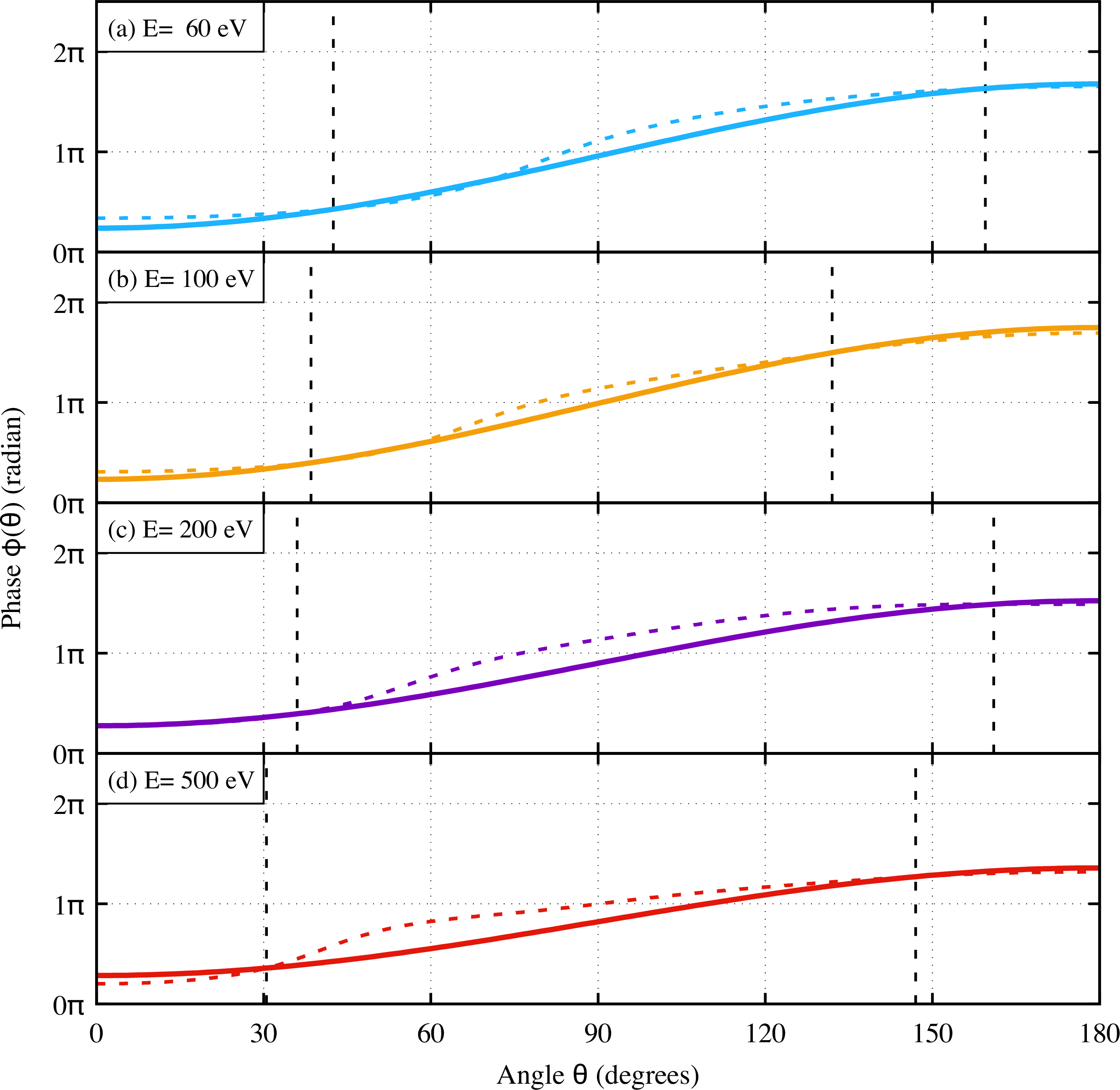
The phase function may further be approximated by a linear function of : . We determine the coefficients and at the equilibrium bond length , and obtain
| (17) | |||
| (18) |
where and are respectively and at the equilibrium bond length.
Figure 3 shows that the phase and the approximate phase function coincide at and . According to figure 1, the most forward valley position moves further forward (i.e. ) and appears around when elongating the bond length . The phase function depends on the scattering potential of scattering site of carbon, and the change of the potential with the bond elongation is negligible in the high energy regime. Based on these facts and the agreement between the numerically calculated phase and the approximate phase function shown in figure 3, we expect this approximation of the phase to be still valid after the elongation of the bond length .
Applying the approximation above to equation 16, we obtain finally the equation,
| (19) |
where , depends on and is not sensitive to . This equation describes the relationship between the bond length and the peak or valley positions of the PA-MFPADs. It has a form similar to Young’s formula in equation 6, but the numerator differs by and a constant shift appears, due to the angle dependency of the phase . In the next section, we will give a physical interpretation of this difference between equation 19 and the ordinary Young’s formula.
3 Results and Discussion
3.1 Extracting bond length information from PA-MFPADs by using our new formula for - interference
Here, we consider an experimental procedure to determine the evolution of the bond length of diatomic molecules. Since the parameter is almost independent of the bond length, once is obtained from the PA-MFPADs with known bond length (e.g., equilibrium state or pre-dissociation structure), we can extract the bond length from the PA-MFPADs obtained with subsequent time evolution. Using this strategy, the bond length can be practically evaluated as a function of the pump-probe delay time using equation 19.
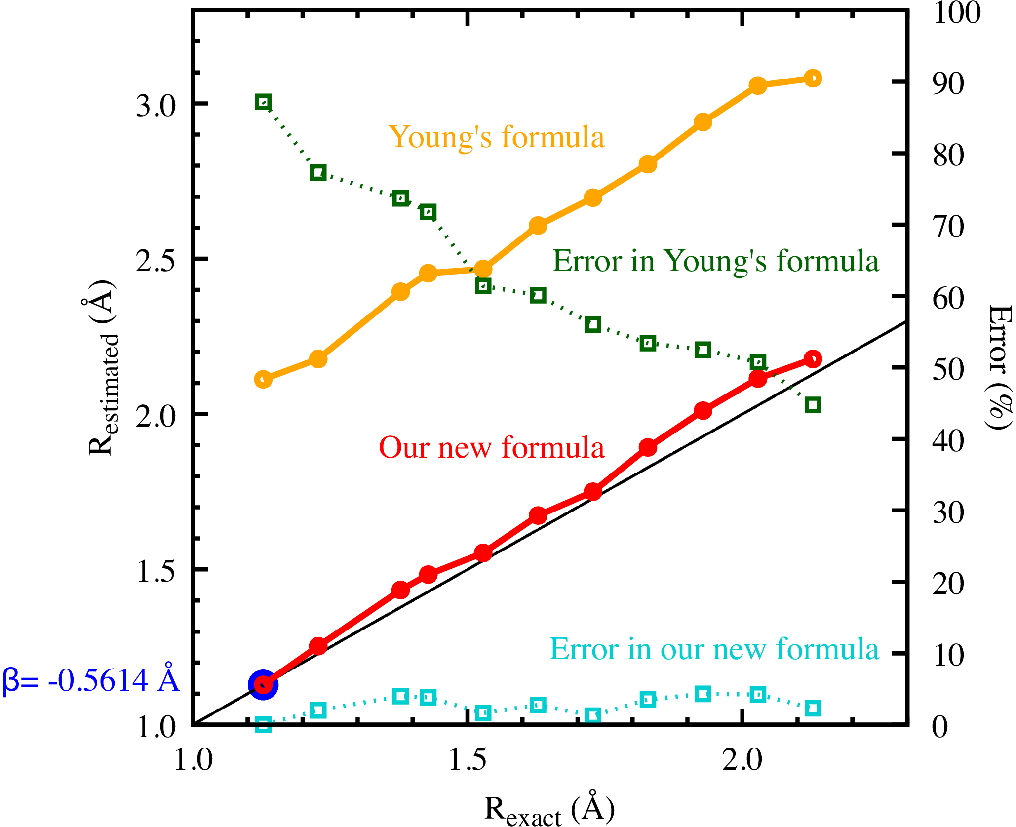
Figure 4 shows the estimated bond lengths against the exact bond lengths . The estimations were performed by using: (i) our new formula in equation 19 and (ii) the ordinary Young’s formula in equation 6 where , , and were chosen, for the set of PA-MFPADs shown in figure 1, which were calculated with the FPMS method at the photoelectron energy eV (). The parameter was evaluated as -0.5614 Å so as to make and agree at the equilibrium bond length Å. The bond lengths were estimated with less than a 5 % error by using our new formula, whereas the conventional Young’s formula gives an estimated error of more than 50 %. From these results we confirm that our new formula (equation 19) for - wave interference works very well for a wide range of bond lengths, and therefore can be considered to be more or less universal. One may notice that, in figure 4, if the Young’s formula is shifted down by to cross the equilibrium bond length (a large blue dot):
| (20) |
then equation 20 also fits to the black line well, though there is no physical background of shifting the Young’s formula by . The reason why this artificial shift also works may be understood because, from equations 19 and 20, the shift may be given by , with and being at the equilibrium bond length , and are nearly constant () as long as and are selected to be the closest to and 0, respectively, as shown in figure 1.
The estimation obtained with our new formula, shown in figure 4 as a red line, exhibits a small deviation from the black , which oscillates as a function of . This deviation is due to the linear fitting of the phase by a cosine function, as shown in figure 4. This fitting is done so that both functions match at and . As the bond length elongates, the positions of and change and move away from and , so that the errors in our approximation increase. While keeps moving away from as the bond length increases, the difference between and oscillates as a function of the bond length due to the appearance of a new peak or valley. This results in oscillations in the estimated error.
There is an additional error due to the truncation of the Multiple Scattering series at first order. Considering that the effect of higher order scattering is not negligible for shorter bond lengths, and that our new formula was derived on the basis of the single scattering approximation, one would expect longer bond lengths to give better estimations. Contraryly to this expectation, figure 4 shows that the agreement between and becomes worse as the bond length increases. This result is due to the fact that the parameter was evaluated at the shortest bond length which is implicitly affected by higher order scattering effects.
3.2 Using simple wave mechanics to interpret the origin of the difference between Young’s formula and our new formula
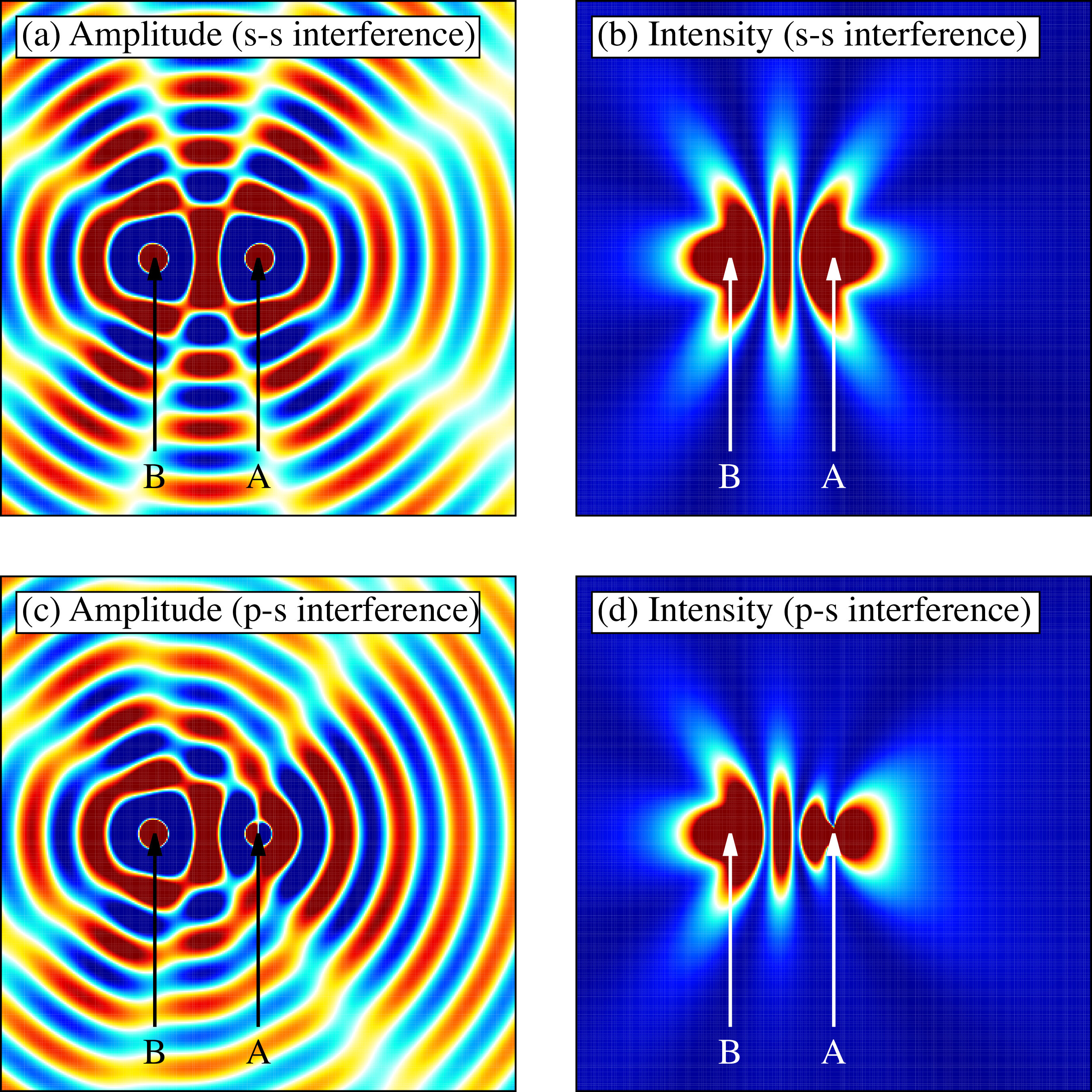
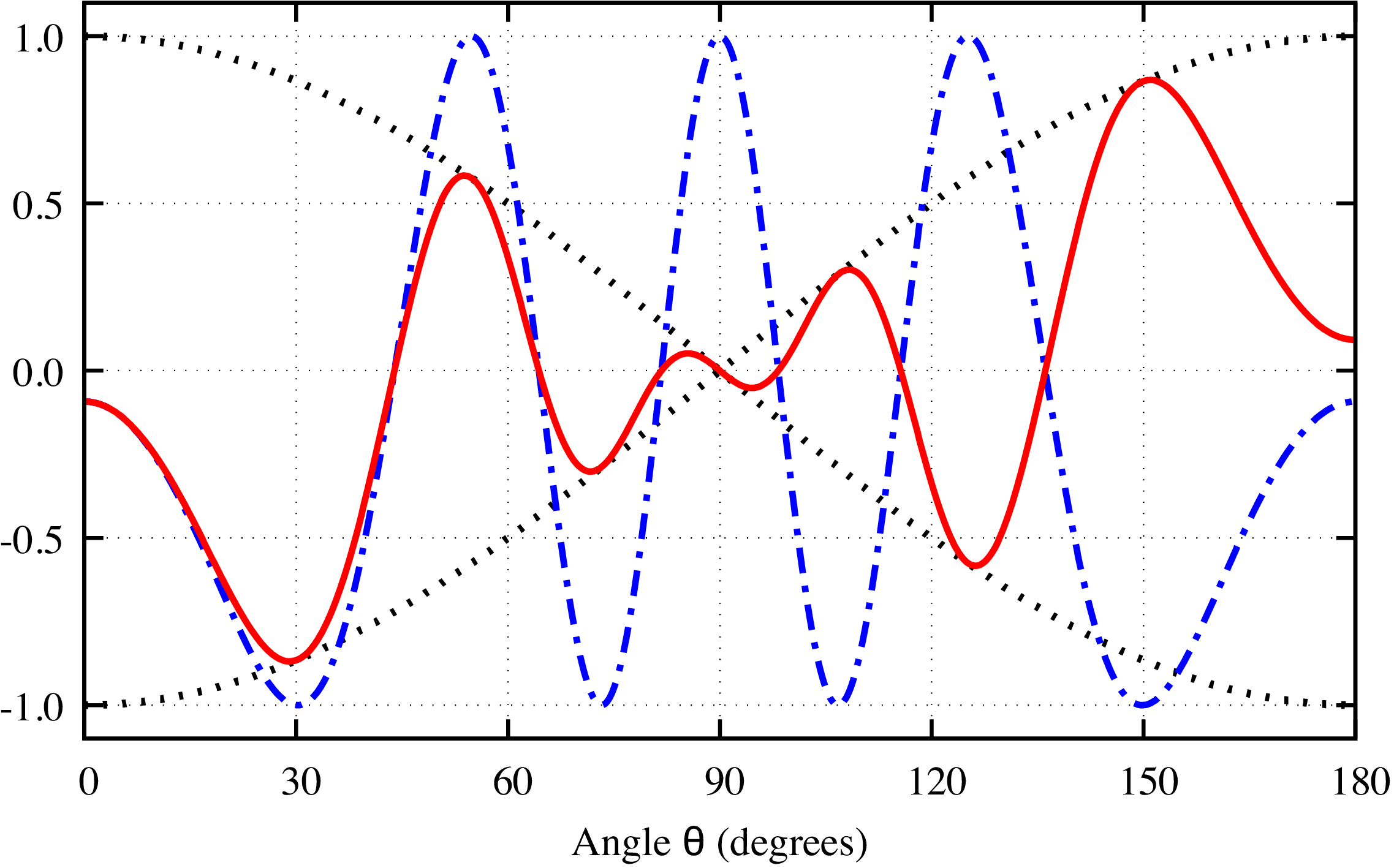
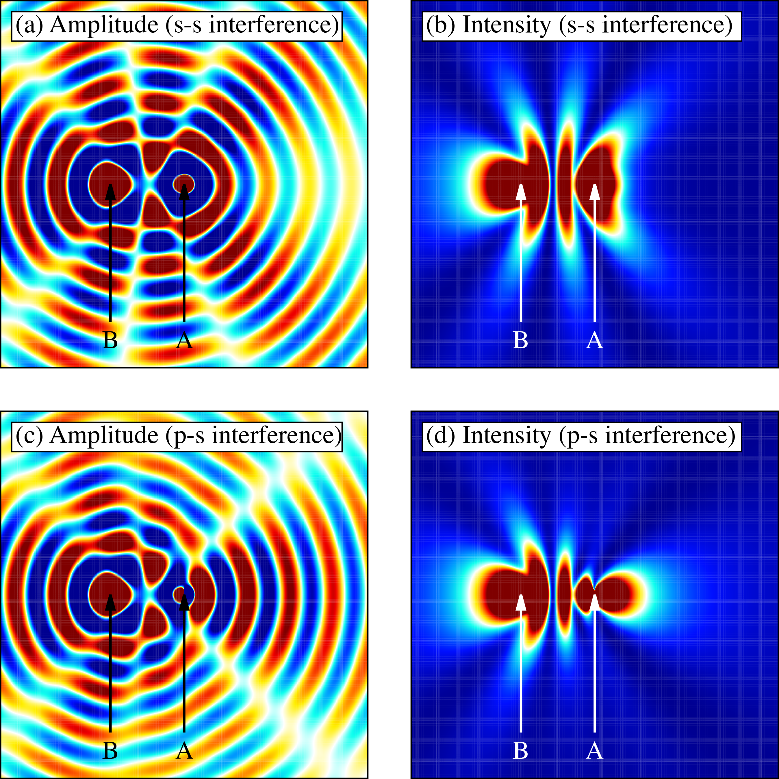
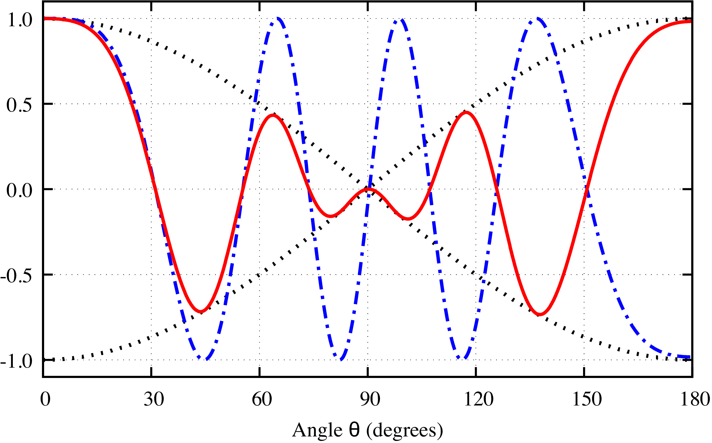
From a physical point of view, the difference between Young’s double-slit experiment and PA-MFPADs is that the flower shape pattern in PA-MFPADs is mainly composed of interferences between a -wave (directly excited dipole wave originating from the atom absorbing the X-ray) and an -wave (wave singly scattered from the neighboring atom). On the other hand, Young’s double-slit experiment is composed of interferences between an -wave and another -wave. Figures 5-8 show the - and - interferences using a very simple model in which the -wave is and the -wave is . The difference between figures 5-6 and figures 7-8 is that in the latter, we have incorporated a plane wave propagation , where , for the photoelectron wave going from point A to point B. In figure 5, either an - or a -wave are emitted from point source A and the -wave from point source B, respectively. By contrast, in figure 7, either an - or a -wave is emitted from point source A, then propagates to point B and is finally scattered, the scattered -wave being emitted from point source B. As can be seen from Figures 6 and 8, the difference between the - interference and the - interference appears as a cosine envelope, which makes the number of peaks/valleys differ by one, due to the change of sign of the -wave at . This is the reason why the numerator of the first term in equation 6 is , while it is in equation 19. In the high energy regime, becomes so large that and the energy-dependent parameter becomes negligible, making our new formula for - interference converge to the ordinary Young’s formula for - interference.
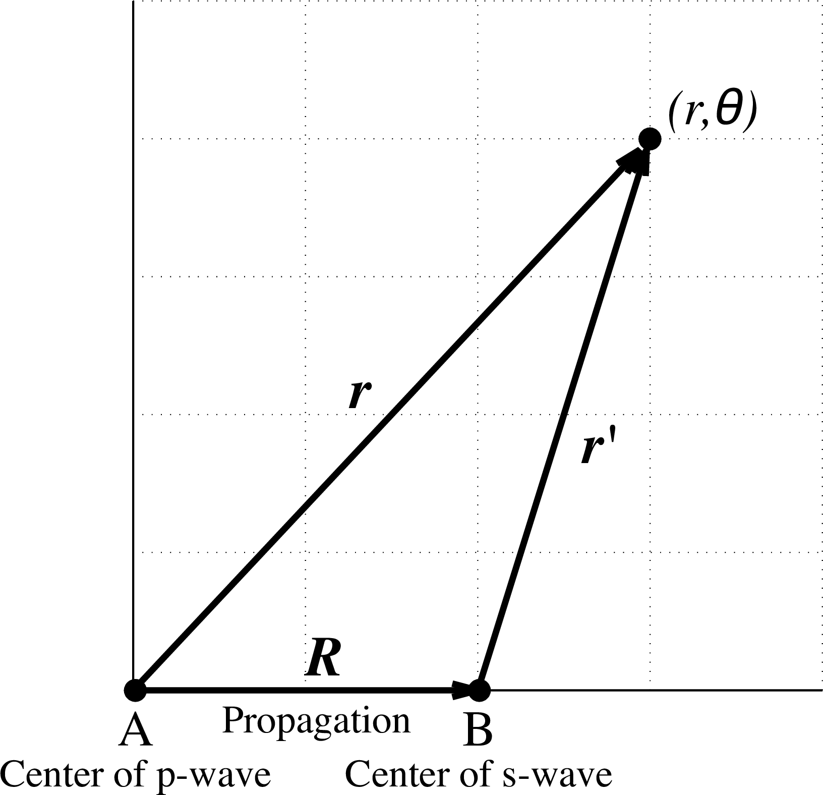
Now, we formulate the intensity observed at the point for the - interference by considering the propagation in the form of a plane wave (see the schematic diagram of the model shown in figure 9). The intensity is given as
In the limit and ,
and the intensity of the interference of a -wave and an -wave separated by reduces to
Thus, the fringes caused by the - interference are given by the last term which agrees with the expression for the PA-MFPADs interference term given in equation 9, except for the phase of the scattering amplitude. Therefore, the fringes of PA-MFPADs can be interpreted as the result of interferences between the -wave, which is excited along the molecular axis and propagates as a plane wave to the neighboring atoms, and the scattered -wave, whose phase is shifted by .
4 Conclusions
We have derived a new formula, equation 19, to describe the interference patterns that appear as a flower shape in PA-MFPADs of hetero-diatomic molecules within the framework of Multiple Scattering theory, using (i) the single scattering approximation, (ii) the Plane Wave approximation, and (iii) the Muffin-tin approximation.
As the new equation was derived by assuming , it works well for fringes close to the forward or the backward direction. Thus, choosing two angles, one at the fringe nearest to the forward direction and the second at the last fringe closest to the backward direction, we are able to reduce the theoretical errors in our approximation of the phase of the scattering amplitude. For practical use, the choice of peaks/valleys in our new formula is one of the key points for a secure analysis of experimental results. As can be seen from figure 1, the peaks and valleys appearing near the molecular-axis perpendicular direction have a more complex structure than those appearing in the forward or backward direction. Furthermore, as the photoelectron kinetic energy or bond length increases, the number of peaks and valleys increases (see equation 9), which makes it difficult to distinguish fringes from each other for middle-range angles. For this reason, the choice of two angles, one at the fringe nearest to the forward direction and the second at the last fringe closest to the backward direction, allows us to perform the analysis with less experimental ambiguity.
The accuracy of this new bond length prediction equation was benchmarked against PA-MFPADs of CO2+ molecule calculated theoretically using the Full-potential method. We found the relative error to be surprisingly very small, i.e., less than 5%. This encourages us to utilize this new formula to obtain bond length information of hetero-diatomic molecules on dissociation dynamics through time-resolved PA-MFPADs using the COLTRIMS-Reaction Microscope and the two-color XFEL pump-probe set-up.
Thanks to Multiple Scattering theory, the physical mechanism behind the flower shape pattern in PA-MFPADs has been revealed, and the errors originating from the use of the Young’s formula (equation 6) to model the flower shape has been clarified. We have pointed out that the additional node appearing in the flower shape is due to the reversal of the sign of the direct dipole wave, i.e. a -wave from absorbing atom at . Because of this effect, we should have an error in the parameter in Young’s formula in equation 6 when and , and we should subtract in the numerator. In addition, the parameter , which is not included in Young’s formula, needs to be introduced. This parameter depends on the kinetic energy of the photoelectrons. It is not sensitive to the bond length, and contains information on the difference in phase of the scattered waves at the angles of the two selected fringes.
In nature, a similar phenomenon of interference between -waves and -waves occurs within wave mechanics. We believe that the newly derived formula for -wave and -wave interferences can be applied not only for PA-MFPADs but also in other fields of science.
Acknowledgements
This work was performed under the Cooperative Research Program of “Network Joint Research Center for Materials and Devices”. K.H. acknowledges funding by JST CREST Grant No. JPMJCR1861 and JSPS KAKENHI under Grant No. 18K05027 and 17K04980. K. Y. is grateful for the financial support from Building of Consortia for the Development of Human Resources in Science and Technology, MEXT, and JSPS KAKENHI Grant Number 19H05628.
References
References
- [1] Ahmed H. Zewail. Femtochemistry: atomic-scale dynamics of the chemical bond. The Journal of Physical Chemistry A, 104(24):5660–5694, May 2000.
- [2] Ahmed H. Zewail. Femtochemistry: Atomic-scale dynamics of the chemical bond using ultrafast lasers (nobel lecture). Angewandte Chemie International Edition, 39(15):2586–2631, 2000.
- [3] Ahmed H. Zewail. 4D visualization of matter: recent collected works. Imperial College Press, London, 2014. OCLC: ocn880965090.
- [4] W. Ackermann, G. Asova, V. Ayvazyan, A. Azima, N. Baboi, J. Bähr, V. Balandin, B. Beutner, A. Brandt, A. Bolzmann, R. Brinkmann, O. I. Brovko, M. Castellano, P. Castro, L. Catani, E. Chiadroni, S. Choroba, A. Cianchi, J. T. Costello, D. Cubaynes, J. Dardis, W. Decking, H. Delsim-Hashemi, A. Delserieys, G. Di Pirro, M. Dohlus, S. Düsterer, A. Eckhardt, H. T. Edwards, B. Faatz, J. Feldhaus, K. Flöttmann, J. Frisch, L. Fröhlich, T. Garvey, U. Gensch, Ch. Gerth, M. Görler, N. Golubeva, H.-J. Grabosch, M. Grecki, O. Grimm, K. Hacker, U. Hahn, J. H. Han, K. Honkavaara, T. Hott, M. Hüning, Y. Ivanisenko, E. Jaeschke, W. Jalmuzna, T. Jezynski, R. Kammering, V. Katalev, K. Kavanagh, E. T. Kennedy, S. Khodyachykh, K. Klose, V. Kocharyan, M. Körfer, M. Kollewe, W. Koprek, S. Korepanov, D. Kostin, M. Krassilnikov, G. Kube, M. Kuhlmann, C. L. S. Lewis, L. Lilje, T. Limberg, D. Lipka, F. Löhl, H. Luna, M. Luong, M. Martins, M. Meyer, P. Michelato, V. Miltchev, W. D. Möller, L. Monaco, W. F. O. Müller, O. Napieralski, O. Napoly, P. Nicolosi, D. Nölle, T. Nuñez, A. Oppelt, C. Pagani, R. Paparella, N. Pchalek, J. Pedregosa-Gutierrez, B. Petersen, B. Petrosyan, G. Petrosyan, L. Petrosyan, J. Pflüger, E. Plönjes, L. Poletto, K. Pozniak, E. Prat, D. Proch, P. Pucyk, P. Radcliffe, H. Redlin, K. Rehlich, M. Richter, M. Roehrs, J. Roensch, R. Romaniuk, M. Ross, J. Rossbach, V. Rybnikov, M. Sachwitz, E. L. Saldin, W. Sandner, H. Schlarb, B. Schmidt, M. Schmitz, P. Schmüser, J. R. Schneider, E. A. Schneidmiller, S. Schnepp, S. Schreiber, M. Seidel, D. Sertore, A. V. Shabunov, C. Simon, S. Simrock, E. Sombrowski, A. A. Sorokin, P. Spanknebel, R. Spesyvtsev, L. Staykov, B. Steffen, F. Stephan, F. Stulle, H. Thom, K. Tiedtke, M. Tischer, S. Toleikis, R. Treusch, D. Trines, I. Tsakov, E. Vogel, T. Weiland, H. Weise, M. Wellhöfer, M. Wendt, I. Will, A. Winter, K. Wittenburg, W. Wurth, P. Yeates, M. V. Yurkov, I. Zagorodnov, and K. Zapfe. Operation of a free-electron laser from the extreme ultraviolet to the water window. Nature Photonics, 1(6):336–342, June 2007.
- [5] P. Emma, R. Akre, J. Arthur, R. Bionta, C. Bostedt, J. Bozek, A. Brachmann, P. Bucksbaum, R. Coffee, F.-J. Decker, Y. Ding, D. Dowell, S. Edstrom, A. Fisher, J. Frisch, S. Gilevich, J. Hastings, G. Hays, Ph. Hering, Z. Huang, R. Iverson, H. Loos, M. Messerschmidt, A. Miahnahri, S. Moeller, H.-D. Nuhn, G. Pile, D. Ratner, J. Rzepiela, D. Schultz, T. Smith, P. Stefan, H. Tompkins, J. Turner, J. Welch, W. White, J. Wu, G. Yocky, and J. Galayda. First lasing and operation of an Ångstrom-wavelength free-electron laser. Nature Photonics, 4:641–647, 2010.
- [6] Tetsuya Ishikawa, Hideki Aoyagi, Takao Asaka, Yoshihiro Asano, Noriyoshi Azumi, Teruhiko Bizen, Hiroyasu Ego, Kenji Fukami, Toru Fukui, Yukito Furukawa, Shunji Goto, Hirofumi Hanaki, Toru Hara, Teruaki Hasegawa, Takaki Hatsui, Atsushi Higashiya, Toko Hirono, Naoyasu Hosoda, Miho Ishii, Takahiro Inagaki, Yuichi Inubushi, Toshiro Itoga, Yasumasa Joti, Masahiro Kago, Takashi Kameshima, Hiroaki Kimura, Yoichi Kirihara, Akio Kiyomichi, Toshiaki Kobayashi, Chikara Kondo, Togo Kudo, Hirokazu Maesaka, Xavier M. Maréchal, Takemasa Masuda, Shinichi Matsubara, Takahiro Matsumoto, Tomohiro Matsushita, Sakuo Matsui, Mitsuru Nagasono, Nobuteru Nariyama, Haruhiko Ohashi, Toru Ohata, Takashi Ohshima, Shun Ono, Yuji Otake, Choji Saji, Tatsuyuki Sakurai, Takahiro Sato, Kei Sawada, Takamitsu Seike, Katsutoshi Shirasawa, Takashi Sugimoto, Shinsuke Suzuki, Sunao Takahashi, Hideki Takebe, Kunikazu Takeshita, Kenji Tamasaku, Hitoshi Tanaka, Ryotaro Tanaka, Takashi Tanaka, Tadashi Togashi, Kazuaki Togawa, Atsushi Tokuhisa, Hiromitsu Tomizawa, Kensuke Tono, Shukui Wu, Makina Yabashi, Mitsuhiro Yamaga, Akihiro Yamashita, Kenichi Yanagida, Chao Zhang, Tsumoru Shintake, Hideo Kitamura, and Noritaka Kumagai. A compact x-ray free-electron laser emitting in the sub-ångström region. Nature Photonics, 6(8):540–544, June 2012.
- [7] E Allaria, A Battistoni, F Bencivenga, R Borghes, C Callegari, F Capotondi, D Castronovo, P Cinquegrana, D Cocco, M Coreno, P Craievich, R Cucini, F D’Amico, M B Danailov, A Demidovich, G De Ninno, A Di Cicco, S Di Fonzo, M Di Fraia, S Di Mitri, B Diviacco, W M Fawley, E Ferrari, A Filipponi, L Froehlich, A Gessini, E Giangrisostomi, L Giannessi, D Giuressi, C Grazioli, R Gunnella, R Ivanov, B Mahieu, N Mahne, C Masciovecchio, I P Nikolov, G Passos, E Pedersoli, G Penco, E Principi, L Raimondi, R Sergo, P Sigalotti, C Spezzani, C Svetina, M Trovò, and M Zangrando. Tunability experiments at the FERMI@elettra free-electron laser. New Journal of Physics, 14(11):113009, nov 2012.
- [8] Heung-Sik Kang, Chang-Ki Min, Hoon Heo, Changbum Kim, Haeryong Yang, Gyujin Kim, Inhyuk Nam, Soung Youl Baek, Hyo-Jin Choi, Geonyeong Mun, Byoung Ryul Park, Young Jin Suh, Dong Cheol Shin, Jinyul Hu, Juho Hong, Seonghoon Jung, Sang-Hee Kim, KwangHoon Kim, Donghyun Na, Soung Soo Park, Yong Jung Park, Jang-Hui Han, Young Gyu Jung, Seong Hun Jeong, Hong Gi Lee, Sangbong Lee, Sojeong Lee, Woul-Woo Lee, Bonggi Oh, Hyung Suck Suh, Yong Woon Parc, Sung-Ju Park, Min Ho Kim, Nam-Suk Jung, Young-Chan Kim, Mong-Soo Lee, Bong-Ho Lee, Chi-Won Sung, Ik-Su Mok, Jung-Moo Yang, Chae-Soon Lee, Hocheol Shin, Ji Hwa Kim, Yongsam Kim, Jae Hyuk Lee, Sang-Youn Park, Jangwoo Kim, Jaeku Park, Intae Eom, Seungyu Rah, Sunam Kim, Ki Hyun Nam, Jaehyun Park, Jaehun Park, Sangsoo Kim, Soonam Kwon, Sang Han Park, Kyung Sook Kim, Hyojung Hyun, Seung Nam Kim, Seonghan Kim, Sun min Hwang, Myong Jin Kim, Chae yong Lim, Chung-Jong Yu, Bong-Soo Kim, Tai-Hee Kang, Kwang-Woo Kim, Seung-Hwan Kim, Hee-Seock Lee, Heung-Soo Lee, Ki-Hyeon Park, Tae-Yeong Koo, Dong-Eon Kim, and In Soo Ko. Hard x-ray free-electron laser with femtosecond-scale timing jitter. Nature Photonics, 11(11):708–713, October 2017.
- [9] W. Decking, S. Abeghyan, P. Abramian, A. Abramsky, A. Aguirre, C. Albrecht, P. Alou, M. Altarelli, P. Altmann, K. Amyan, V. Anashin, E. Apostolov, K. Appel, D. Auguste, V. Ayvazyan, S. Baark, F. Babies, N. Baboi, P. Bak, V. Balandin, R. Baldinger, B. Baranasic, S. Barbanotti, O. Belikov, V. Belokurov, L. Belova, V. Belyakov, S. Berry, M. Bertucci, B. Beutner, A. Block, M. Blöcher, T. Böckmann, C. Bohm, M. Böhnert, V. Bondar, E. Bondarchuk, M. Bonezzi, P. Borowiec, C. Bösch, U. Bösenberg, A. Bosotti, R. Böspflug, M. Bousonville, E. Boyd, Y. Bozhko, A. Brand, J. Branlard, S. Briechle, F. Brinker, S. Brinker, R. Brinkmann, S. Brockhauser, O. Brovko, H. Brück, A. Brüdgam, L. Butkowski, T. Büttner, J. Calero, E. Castro-Carballo, G. Cattalanotto, J. Charrier, J. Chen, A. Cherepenko, V. Cheskidov, M. Chiodini, A. Chong, S. Choroba, M. Chorowski, D. Churanov, W. Cichalewski, M. Clausen, W. Clement, C. Cloué, J. A. Cobos, N. Coppola, S. Cunis, K. Czuba, M. Czwalinna, B. D’Almagne, J. Dammann, H. Danared, A. de Zubiaurre Wagner, A. Delfs, T. Delfs, F. Dietrich, T. Dietrich, M. Dohlus, M. Dommach, A. Donat, X. Dong, N. Doynikov, M. Dressel, M. Duda, P. Duda, H. Eckoldt, W. Ehsan, J. Eidam, F. Eints, C. Engling, U. Englisch, A. Ermakov, K. Escherich, J. Eschke, E. Saldin, M. Faesing, A. Fallou, M. Felber, M. Fenner, B. Fernandes, J. M. Fernández, S. Feuker, K. Filippakopoulos, K. Floettmann, V. Fogel, M. Fontaine, A. Francés, I. Freijo Martin, W. Freund, T. Freyermuth, M. Friedland, L. Fröhlich, M. Fusetti, J. Fydrych, A. Gallas, O. García, L. Garcia-Tabares, G. Geloni, N. Gerasimova, C. Gerth, P. Geßler, V. Gharibyan, M. Gloor, J. Głowinkowski, A. Goessel, Z. Gołȩbiewski, N. Golubeva, W. Grabowski, W. Graeff, A. Grebentsov, M. Grecki, T. Grevsmuehl, M. Gross, U. Grosse-Wortmann, J. Grünert, S. Grunewald, P. Grzegory, G. Feng, H. Guler, G. Gusev, J. L. Gutierrez, L. Hagge, M. Hamberg, R. Hanneken, E. Harms, I. Hartl, A. Hauberg, S. Hauf, J. Hauschildt, J. Hauser, J. Havlicek, A. Hedqvist, N. Heidbrook, F. Hellberg, D. Henning, O. Hensler, T. Hermann, A. Hidvégi, M. Hierholzer, H. Hintz, F. Hoffmann, Markus Hoffmann, Matthias Hoffmann, Y. Holler, M. Hüning, A. Ignatenko, M. Ilchen, A. Iluk, J. Iversen, J. Iversen, M. Izquierdo, L. Jachmann, N. Jardon, U. Jastrow, K. Jensch, J. Jensen, M. Jeżabek, M. Jidda, H. Jin, N. Johansson, R. Jonas, W. Kaabi, D. Kaefer, R. Kammering, H. Kapitza, S. Karabekyan, S. Karstensen, K. Kasprzak, V. Katalev, D. Keese, B. Keil, M. Kholopov, M. Killenberger, B. Kitaev, Y. Klimchenko, R. Klos, L. Knebel, A. Koch, M. Koepke, S. Köhler, W. Köhler, N. Kohlstrunk, Z. Konopkova, A. Konstantinov, W. Kook, W. Koprek, M. Körfer, O. Korth, A. Kosarev, K. Kosiński, D. Kostin, Y. Kot, A. Kotarba, T. Kozak, V. Kozak, R. Kramert, M. Krasilnikov, A. Krasnov, B. Krause, L. Kravchuk, O. Krebs, R. Kretschmer, J. Kreutzkamp, O. Kröplin, K. Krzysik, G. Kube, H. Kuehn, N. Kujala, V. Kulikov, V. Kuzminych, D. La Civita, M. Lacroix, T. Lamb, A. Lancetov, M. Larsson, D. Le Pinvidic, S. Lederer, T. Lensch, D. Lenz, A. Leuschner, F. Levenhagen, Y. Li, J. Liebing, L. Lilje, T. Limberg, D. Lipka, B. List, J. Liu, S. Liu, B. Lorbeer, J. Lorkiewicz, H. H. Lu, F. Ludwig, K. Machau, W. Maciocha, C. Madec, C. Magueur, C. Maiano, I. Maksimova, K. Malcher, T. Maltezopoulos, E. Mamoshkina, B. Manschwetus, F. Marcellini, G. Marinkovic, T. Martinez, H. Martirosyan, W. Maschmann, M. Maslov, A. Matheisen, U. Mavric, J. Meißner, K. Meissner, M. Messerschmidt, N. Meyners, G. Michalski, P. Michelato, N. Mildner, M. Moe, F. Moglia, C. Mohr, S. Mohr, W. Möller, M. Mommerz, L. Monaco, C. Montiel, M. Moretti, I. Morozov, P. Morozov, D. Mross, J. Mueller, C. Müller, J. Müller, K. Müller, J. Munilla, A. Münnich, V. Muratov, O. Napoly, B. Näser, N. Nefedov, Reinhard Neumann, Rudolf Neumann, N. Ngada, D. Noelle, F. Obier, I. Okunev, J. A. Oliver, M. Omet, A. Oppelt, A. Ottmar, M. Oublaid, C. Pagani, R. Paparella, V. Paramonov, C. Peitzmann, J. Penning, A. Perus, F. Peters, B. Petersen, A. Petrov, I. Petrov, S. Pfeiffer, J. Pflüger, S. Philipp, Y. Pienaud, P. Pierini, S. Pivovarov, M. Planas, E. Pławski, M. Pohl, J. Polinski, V. Popov, S. Prat, J. Prenting, G. Priebe, H. Pryschelski, K. Przygoda, E. Pyata, B. Racky, A. Rathjen, W. Ratuschni, S. Regnaud-Campderros, K. Rehlich, D. Reschke, C. Robson, J. Roever, M. Roggli, J. Rothenburg, E. Rusiński, R. Rybaniec, H. Sahling, M. Salmani, L. Samoylova, D. Sanzone, F. Saretzki, O. Sawlanski, J. Schaffran, H. Schlarb, M. Schlösser, V. Schlott, C. Schmidt, F. Schmidt-Foehre, M. Schmitz, M. Schmökel, T. Schnautz, E. Schneidmiller, M. Scholz, B. Schöneburg, J. Schultze, C. Schulz, A. Schwarz, J. Sekutowicz, D. Sellmann, E. Semenov, S. Serkez, D. Sertore, N. Shehzad, P. Shemarykin, L. Shi, M. Sienkiewicz, D. Sikora, M. Sikorski, A. Silenzi, C. Simon, W. Singer, X. Singer, H. Sinn, K. Sinram, N. Skvorodnev, P. Smirnow, T. Sommer, A. Sorokin, M. Stadler, M. Steckel, B. Steffen, N. Steinhau-Kühl, F. Stephan, M. Stodulski, M. Stolper, A. Sulimov, R. Susen, J. Świerblewski, C. Sydlo, E. Syresin, V. Sytchev, J. Szuba, N. Tesch, J. Thie, A. Thiebault, K. Tiedtke, D. Tischhauser, J. Tolkiehn, S. Tomin, F. Tonisch, F. Toral, I. Torbin, A. Trapp, D. Treyer, G. Trowitzsch, T. Trublet, T. Tschentscher, F. Ullrich, M. Vannoni, P. Varela, G. Varghese, G. Vashchenko, M. Vasic, C. Vazquez-Velez, A. Verguet, S. Vilcins-Czvitkovits, R. Villanueva, B. Visentin, M. Viti, E. Vogel, E. Volobuev, R. Wagner, N. Walker, T. Wamsat, H. Weddig, G. Weichert, H. Weise, R. Wenndorf, M. Werner, R. Wichmann, C. Wiebers, M. Wiencek, T. Wilksen, I. Will, L. Winkelmann, M. Winkowski, K. Wittenburg, A. Witzig, P. Wlk, T. Wohlenberg, M. Wojciechowski, F. Wolff-Fabris, G. Wrochna, K. Wrona, M. Yakopov, B. Yang, F. Yang, M. Yurkov, I. Zagorodnov, P. Zalden, A. Zavadtsev, D. Zavadtsev, A. Zhirnov, A. Zhukov, V. Ziemann, A. Zolotov, N. Zolotukhina, F. Zummack, and D. Zybin. A MHz-repetition-rate hard x-ray free-electron laser driven by a superconducting linear accelerator. Nature Photonics, 14(6):391–397, May 2020.
- [10] Christopher J. Milne, Thomas Schietinger, Masamitsu Aiba, Arturo Alarcon, Jürgen Alex, Alexander Anghel, Vladimir Arsov, Carl Beard, Paul Beaud, Simona Bettoni, Markus Bopp, Helge Brands, Manuel Brönnimann, Ingo Brunnenkant, Marco Calvi, Alessandro Citterio, Paolo Craievich, Marta Csatari Divall, Mark Dällenbach, Michael D’Amico, Andreas Dax, Yunpei Deng, Alexander Dietrich, Roberto Dinapoli, Edwin Divall, Sladana Dordevic, Simon Ebner, Christian Erny, Hansrudolf Fitze, Uwe Flechsig, Rolf Follath, Franziska Frei, Florian Gärtner, Romain Ganter, Terence Garvey, Zheqiao Geng, Ishkhan Gorgisyan, Christopher Gough, Andreas Hauff, Christoph P. Hauri, Nicole Hiller, Tadej Humar, Stephan Hunziker, Gerhard Ingold, Rasmus Ischebeck, Markus Janousch, Pavle Juranić, Mario Jurcevic, Maik Kaiser, Babak Kalantari, Roger Kalt, Boris Keil, Christoph Kittel, Gregor Knopp, Waldemar Koprek, Henrik T. Lemke, Thomas Lippuner, Daniel Llorente Sancho, Florian Löhl, Carlos Lopez-Cuenca, Fabian Märki, Fabio Marcellini, Goran Marinkovic, Isabelle Martiel, Ralf Menzel, Aldo Mozzanica, Karol Nass, Gian Luca Orlandi, Cigdem Ozkan Loch, Ezequiel Panepucci, Martin Paraliev, Bruce Patterson, Bill Pedrini, Marco Pedrozzi, Patrick Pollet, Claude Pradervand, Eduard Prat, Peter Radi, Jean-Yves Raguin, Sophie Redford, Jens Rehanek, Julien Réhault, Sven Reiche, Matthias Ringele, Jochen Rittmann, Leonid Rivkin, Albert Romann, Marie Ruat, Christian Ruder, Leonardo Sala, Lionel Schebacher, Thomas Schilcher, Volker Schlott, Thomas Schmidt, Bernd Schmitt, Xintian Shi, Markus Stadler, Lukas Stingelin, Werner Sturzenegger, Jakub Szlachetko, Dhanya Thattil, Daniel M. Treyer, Alexandre Trisorio, Wolfgang Tron, Seraphin Vetter, Carlo Vicario, Didier Voulot, Meitian Wang, Thierry Zamofing, Christof Zellweger, Riccardo Zennaro, Elke Zimoch, Rafael Abela, Luc Patthey, and Hans-Heinrich Braun. Swissfel: The swiss x-ray free electron laser. Applied Sciences, 7(7), 2017.
- [11] Christoph Bostedt, Sébastien Boutet, David M. Fritz, Zhirong Huang, Hae Ja Lee, Henrik T. Lemke, Aymeric Robert, William F. Schlotter, Joshua J. Turner, and Garth J. Williams. Linac coherent light source: The first five years. Rev. Mod. Phys., 88:015007, Mar 2016.
- [12] E A Seddon, J A Clarke, D J Dunning, C Masciovecchio, C J Milne, F Parmigiani, D Rugg, J C H Spence, N R Thompson, K Ueda, S M Vinko, J S Wark, and W Wurth. Short-wavelength free-electron laser sources and science: a review. Reports on Progress in Physics, 80(11):115901, oct 2017.
- [13] Carlo Callegari, Alexei N. Grum-Grzhimailo, Kenichi L. Ishikawa, Kevin C. Prince, Giuseppe Sansone, and Kiyoshi Ueda. Atomic, molecular and optical physics applications of longitudinally coherent and narrow bandwidth free-electron lasers. Physics Reports, 904:1–59, 2021. Atomic, molecular and optical physics applications of longitudinally coherent and narrow bandwidth Free-Electron Lasers.
- [14] J. J. Rehr and R. C. Albers. Theoretical approaches to x-ray absorption fine structure. Rev. Mod. Phys., 72:621–654, Jul 2000.
- [15] D. P. Woodruff. Photoelectron diffraction: from phenomenological demonstration to practical tool. Applied Physics A, 92:439–445, 2008.
- [16] E. Shigemasa, J. Adachi, M. Oura, and A. Yagishita. Angular distributions of photoelectrons from fixed-in-space N2 molecules. Physical Review Letters, 74:359–362, Jan 1995.
- [17] J. Ullrich, R. Moshammer, A. Dorn, R. Dörner, L. Ph. H. Schmidt, and H. Schmidt-Böcking. Recoil-ion and electron momentum spectroscopy: reaction-microscopes. Reports on Progress in Physics, 66(9):1463–1545, aug 2003.
- [18] A. Landers, Th. Weber, I. Ali, A. Cassimi, M. Hattass, O. Jagutzki, A. Nauert, T. Osipov, A. Staudte, M. H. Prior, H. Schmidt-Böcking, C. L. Cocke, and R. Dörner. Photoelectron diffraction mapping: Molecules illuminated from within. Physical Review Letters, 87:013002, Jun 2001.
- [19] J. B. Williams, C. S. Trevisan, M. S. Schöffler, T. Jahnke, I. Bocharova, H. Kim, B. Ulrich, R. Wallauer, F. Sturm, T. N. Rescigno, A. Belkacem, R. Dörner, Th. Weber, C. W. McCurdy, and A. L. Landers. Imaging polyatomic molecules in three dimensions using molecular frame photoelectron angular distributions. Physical Review Letters, 108:233002, Jun 2012.
- [20] Hironobu Fukuzawa, Robert R. Lucchese, Xiao-Jing Liu, Kentaro Sakai, Hiroshi Iwayama, Kiyonobu Nagaya, Katharina Kreidi, Markus S. Schöffler, James R. Harries, Yusuke Tamenori, Yuichiro Morishita, Isao H. Suzuki, Norio Saito, and Kiyoshi Ueda. Probing molecular bond-length using molecular-frame photoelectron angular distributions. The Journal of Chemical Physics, 150(17):174306, 2019.
- [21] A Rouzée, P Johnsson, L Rading, A Hundertmark, W Siu, Y Huismans, S Düsterer, H Redlin, F Tavella, N Stojanovic, A Al-Shemmary, F Lépine, D M P Holland, T Schlatholter, R Hoekstra, H Fukuzawa, K Ueda, and M J J Vrakking. Towards imaging of ultrafast molecular dynamics using FELs. Journal of Physics B: Atomic, Molecular and Optical Physics, 46(16):164029, aug 2013.
- [22] R. Boll, D. Anielski, C. Bostedt, J. D. Bozek, L. Christensen, R. Coffee, S. De, P. Decleva, S. W. Epp, B. Erk, L. Foucar, F. Krasniqi, J. Küpper, A. Rouzée, B. Rudek, A. Rudenko, S. Schorb, H. Stapelfeldt, M. Stener, S. Stern, S. Techert, S. Trippel, M. J. J. Vrakking, J. Ullrich, and D. Rolles. Femtosecond photoelectron diffraction on laser-aligned molecules: Towards time-resolved imaging of molecular structure. Phys. Rev. A, 88:061402, Dec 2013.
- [23] Kyo Nakajima, Takahiro Teramoto, Hiroshi Akagi, Takashi Fujikawa, Takuya Majima, Shinichirou Minemoto, Kanade Ogawa, Hirofumi Sakai, Tadashi Togashi, Kensuke Tono, Shota Tsuru, Ken Wada, Makina Yabashi, and Akira Yagishita. Photoelectron diffraction from laser-aligned molecules with x-ray free-electron laser pulses. Scientific Reports, 5:14065, 2015.
- [24] Shinichirou Minemoto, Takahiro Teramoto, Hiroshi Akagi, Takashi Fujikawa, Takuya Majima, Kyo Nakajima, Kaori Niki, Shigeki Owada, Hirofumi Sakai, Tadashi Togashi, Kensuke Tono, Shota Tsuru, Ken Wada, Makina Yabashi, Shintaro Yoshida, and Akira Yagishita. Structure determination of molecules in an alignment laser field by femtosecond photoelectron diffraction using an X-ray free-electron laser. Scientific Reports, 6:38654, 2016.
- [25] Gregor Kastirke, Markus S. Schöffler, Miriam Weller, Jonas Rist, Rebecca Boll, Nils Anders, Thomas M. Baumann, Sebastian Eckart, Benjamin Erk, Alberto De Fanis, Kilian Fehre, Averell Gatton, Sven Grundmann, Patrik Grychtol, Alexander Hartung, Max Hofmann, Markus Ilchen, Christian Janke, Max Kircher, Maksim Kunitski, Xiang Li, Tommaso Mazza, Niklas Melzer, Jacobo Montano, Valerija Music, Giammarco Nalin, Yevheniy Ovcharenko, Andreas Pier, Nils Rennhack, Daniel E. Rivas, Reinhard Dörner, Daniel Rolles, Artem Rudenko, Philipp Schmidt, Juliane Siebert, Nico Strenger, Daniel Trabert, Isabel Vela-Perez, Rene Wagner, Thorsten Weber, Joshua B. Williams, Pawel Ziolkowski, Lothar Ph. H. Schmidt, Achim Czasch, Florian Trinter, Michael Meyer, Kiyoshi Ueda, Philipp V. Demekhin, and Till Jahnke. Photoelectron diffraction imaging of a molecular breakup using an x-ray free-electron laser. Physical Review X, 10:021052, Jun 2020.
- [26] Svitozar Serkez, Winfried Decking, Lars Froehlich, Natalia Gerasimova, Jan Grünert, Marc Guetg, Marko Huttula, Suren Karabekyan, Andreas Koch, Vitali Kocharyan, and et al. Opportunities for two-color experiments in the soft x-ray regime at the european xfel. Applied Sciences, 10(8):2728, Apr 2020.
- [27] F Ota, K Yamazaki, D Sébilleau, K Ueda, and K Hatada. Theory of polarization-averaged core-level molecular-frame photoelectron angular distributions: I. A full-potential method and its application to dissociating carbon monoxide dication. Journal of Physics B: Atomic, Molecular and Optical Physics, 54(2):024003, January 2021.
- [28] F Ota, K Hatada, D Sébilleau, K Ueda, and K Yamazaki. Theory of polarization-averaged core-level molecular-frame photoelectron angular distributions: II. Extracting the x-ray-induced fragmentation dynamics of carbon monoxide dication from forward and backward intensities. Journal of Physics B: Atomic, Molecular and Optical Physics, 54(8):084001, April 2021.
- [29] J Korringa. On the calculation of the energy of a bloch wave in a metal. Physica, 13(6):392 – 400, 1947.
- [30] W. Kohn and N. Rostoker. Solution of the Schrödinger Equation in Periodic Lattices with an Application to Metallic Lithium. Physical Review, 94:1111–1120, Jun 1954.
- [31] Francesco Aquilante, Jochen Autschbach, Rebecca K. Carlson, Liviu F. Chibotaru, Mickaël G. Delcey, Luca De Vico, Ignacio Fdez. Galván, Nicolas Ferré, Luis Manuel Frutos, Laura Gagliardi, Marco Garavelli, Angelo Giussani, Chad E. Hoyer, Giovanni Li Manni, Hans Lischka, Dongxia Ma, Per Åke Malmqvist, Thomas Müller, Artur Nenov, Massimo Olivucci, Thomas Bondo Pedersen, Daoling Peng, Felix Plasser, Ben Pritchard, Markus Reiher, Ivan Rivalta, Igor Schapiro, Javier Segarra-Martí, Michael Stenrup, Donald G. Truhlar, Liviu Ungur, Alessio Valentini, Steven Vancoillie, Valera Veryazov, Victor P. Vysotskiy, Oliver Weingart, Felipe Zapata, and Roland Lindh. Molcas 8: New capabilities for multiconfigurational quantum chemical calculations across the periodic table. Journal of Computational Chemistry, 37(5):506–541, 2016.
- [32] L. S. Cederbaum, P. Campos, F. Tarantelli, and A. Sgamellotti. Band shape and vibrational structure in auger spectra: Theory and application to carbon monoxide. The Journal of Chemical Physics, 95(9):6634–6644, 1991.
- [33] Didier Sébilleau, Calogero Natoli, George M. Gavaza, Haifeng Zhao, Fabiana Da Pieve, and Keisuke Hatada. Msspec-1.0: A multiple scattering package for electron spectroscopies in material science. Computer Physics Communications, 182(12):2567 – 2579, 2011.