Theory of polariton-electron interactions in semiconductor microcavities
Abstract
We develop a microscopic description of an electron-doped two-dimensional semiconductor embedded in a microcavity. Specifically, we investigate the interactions between exciton-polaritons and electrons for the case where the interactions between charges are strongly screened and the system is spin polarized. As a starting point, we obtain an analytic expression for the exciton-polariton wave function, and we relate the microscopic parameters of the light-matter system to experimentally measurable quantities, such as the Rabi coupling and the cavity photon frequency. We then derive the polariton-electron interaction within the standard Born approximation and compare it with the exact polariton-electron scattering matrix that we obtain from a diagrammatic approach that has proven highly successful in the context of nuclear physics and ultracold atomic gases. In particular, we show that the Born approximation provides an upper bound on the polariton-electron coupling strength at vanishing momentum. Using our exact microscopic calculation, we demonstrate that polariton-electron scattering can be strongly enhanced compared to the exciton-electron case, which is the opposite of that expected from the Born approximation. We furthermore expose a resonance-like peak at scattering momenta near the polariton inflection point, whose size is set by the strength of the light-matter coupling. Our results arise from the non-Galilean nature of the polariton system and should thus be applicable to a range of semiconductor microcavities such as GaAs quantum wells and atomically thin materials.
I Introduction
By embedding a two-dimensional (2D) semiconductor in a microcavity, one can achieve a strong coupling between photons and bound electron-hole pairs (i.e., excitons). This in turn gives rise to exciton-polaritons, quasiparticles which are superpositions of both light and matter [1, 2, 3]. A key advantage of polaritons over ordinary photons is that they can pairwise interact with other particles via their excitonic component, which is important for a range of applications including polariton superfluidity [4, 5], ultra-fast polariton spin switching [6], and the generation of photon correlations [7, 8]. Moreover, there is the prospect of enhancing the interactions in the polariton system by coupling to few-body bound states such as biexcitons [9] or trions [10].
Interaction processes involving polaritons are conventionally described using the Born approximation [11, 12, 13, 14, 15]. This can essentially be viewed as a two step process. First, the matter component interactions are calculated within the Born approximation, and then the result is weighted by the matter fraction of the involved particles since only this component interacts. There have been various attempts [11, 16, 17, 18, 19] to obtain perturbative corrections beyond the standard Born approximation to include higher-order effects due to the light-matter coupling. However, until now there have been no exact microscopic calculations of few-body processes that involve the constituent electron-hole-photon components of the polaritons, which is mainly due to the complexity associated with treating both the electronic and the light-matter interactions. It is therefore an open and important question whether the assumptions in the Born approximation are valid even at a qualitative level.
In this paper, which accompanies Ref. [20], we use a microscopic model that explicitly includes electrons, holes, and photons to investigate this question. The key simplification is to consider strongly screened electronic interactions. Such a simplified model has previously been used to theoretically investigate the crossover from a Bose-Einstein condensate (BEC) of polaritons to the Bardeen-Cooper-Schrieffer regime of electron-hole superfluidity [21, 22, 23]. Here we show that this approximation allows us to formulate a diagrammatic approach where we can analytically obtain the polariton wave function and propagator, as well as the associated spectrum and photon and exciton fractions. Our resulting microscopic description of exciton-polaritons complements our previous results for Coulomb electronic interactions [24], and it can act as a starting point for further few- and many-body calculations within the model of strongly screened electronic interactions.
We then apply our diagrammatic approach to perform the first exact calculation of spin-polarized polariton-electron scattering within a microscopic model. Importantly, we find that the polariton-electron scattering is strongly enhanced up to the polariton dispersion inflection point compared with exciton-electron scattering, in stark contrast to the assumptions of the Born approximation. We argue that this unexpected feature is because the light-matter coupling shifts the collision energy, which has a stronger effect than the reduction in the interaction strength due the reduced exciton fraction of the polariton. Given that this argument relies only on standard 2D scattering theory [25] which is valid also for unscreened electronic interactions, we expect the enhanced polariton-electron interactions to be a generic feature of 2D semiconductors embedded in microcavities, and we expect our results to be quite accurate even at a quantitative level in the case of more realistic electronic interactions.
Of particular interest is the scattering at low momentum, due to the potential implications for polariton BECs [26] in charge-doped semiconductors. It is well known [27] that the scattering of 2D quantum particles with short range interactions approaches zero logarithmically with momentum. In the case of exciton-electron scattering, the relevant momentum scale is the inverse exciton Bohr radius. Remarkably, in the case of polariton-electron scattering, we find that the resulting momentum scale is suppressed exponentially by the large electron-photon mass ratio, and consequently the polariton-electron scattering only approaches zero in systems that greatly exceed the size of the universe. This is a striking consequence of the polariton being formed from a superposition of particles with extremely different masses, and it allows us to define a finite coupling constant at vanishing momentum.
We furthermore find that the Born approximation severely overestimates the polariton-electron interaction constant for typical experimental parameters. We argue that this is because the Born approximation represents an upper bound on the interaction constant. While this implies that this simple approximation cannot in general be trusted, we show that it can be replaced by a similarly simple expression that calculates the interaction constant instead from the low-energy exciton-electron scattering amplitude, which represents an excellent approximation in the case of a transition metal dichalcogenide (TMD) monolayer or a single GaAs quantum well embedded in a microcavity.
The paper is organized as follows. In Sec. II, we present the microscopic description of a single polariton, taking care to appropriately renormalize the model. We obtain analytic expressions for the polariton wave function, spectrum, and excitonic and photonic fractions, and demonstrate that our results can be obtained within both an operator and a diagrammatic approach. In Sec. III we outline the Born approximation of polariton-electron scattering, which provides an upper bound for our exact calculation presented in Sec. IV. We discuss how our results depend on system parameters relevant to both semiconductor quantum wells and atomically thin semiconductors. In Sec. V we conclude. Technical details are given in the appendices.
II Theoretical description of exciton-polaritons
We consider a system consisting of spin-polarized electrons, holes, and photons in a 2D semiconductor, such as a quantum well or an atomically thin transition metal dichalcogenide material. The Hamiltonian reads
| (1) |
The first line describes the kinetic energies of the particles, where , , and are electron, hole, and photon annihilation operators, respectively, with momentum and kinetic energy , and corresponding masses , , and . is the cavity photon frequency measured from the bandgap. In the second line, we have the electron-hole interactions, which we take to be strongly screened contact interactions of strength . Note that there are no electron-electron or hole-hole interactions in this screened case since the interactions between identical fermions formally vanish due to Pauli exclusion. The last term corresponds to the creation (annihilation) of an electron-hole pair through the absorption (emission) of a photon within the rotating wave approximation, and denotes the strength of the (unrenormalized) light-matter coupling. This term explicitly breaks Galilean invariance by coupling the light photon with much heavier matter particles, which has important consequences for the few-body properties of the system. Note that here and in the following we adopt units where and the system area .
The Hamiltonian contains the bare parameters and that describe the strength of matter-matter and light-matter contact interactions, respectively. We take these to be constant up to an ultraviolet momentum cutoff which is set by the detailed band structure of the 2D semiconductor. For our discussion of polariton physics, the precise value of the momentum cutoff will be irrelevant, since we aim to develop a low-energy theory that is independent of the short-distance physics [24]. Therefore, both and need to be renormalized such that all observable quantities are independent of the momentum cutoff. For simplicity, we take the cutoffs related to and to be the same, denoted , since they both drop out after the renormalization.
II.1 Exciton problem
Let us first discuss how the formation of an exciton is described within the contact interaction model (II). To this end, we consider the most general state of an electron-hole pair with zero center-of-mass momentum:
| (2) |
with the normalization condition Here, is the electron-hole vacuum. In the absence of coupling to light, i.e., at , the wave function satisfies the Schrödinger equation
| (3) |
where we define the electron-hole kinetic energy with the electron-hole reduced mass.
Equation (3) admits a single bound state with binding energy , corresponding to the exciton state (see, e.g., Ref. [28]), which has the associated effective Bohr radius . The corresponding wave function satisfies the equation
| (4) |
Importantly, the right hand side of Eq. (4) does not depend on momentum, and therefore we immediately find that the exciton has the wave function
| (5) |
where comes from the normalization condition
| (6) |
Equation (4) also allows us to relate the bare coupling constant, , to : Acting with the operator on Eq. (4), we find
| (7) |
Here, the sum on is logarithmically divergent, and we have therefore explicitly introduced the ultraviolet momentum cutoff . Once the coupling constant and are related to the exciton binding energy via Eq. (7), all dependence on these bare parameters is eliminated from the problem [28].
It is instructive to compare the operator formalism described above for the exciton problem with the electron-hole matrix [28]:
| (8) |
This is discussed further below in Sec. II.3. In this formalism, the bound state emerges as a pole at the negative energy , where the presence of the infinitesimal positive imaginary part shifts the pole slightly into the lower half of the complex plane. In the vicinity of the pole, we expand the matrix to find . Thus, the normalization naturally emerges in both approaches.
II.2 Operator approach to exciton-polaritons
Let us now discuss how to obtain the polariton spectrum within the model (II), and how to relate this to experimentally measurable quantities. As we will show, the Hamiltonian (II) is analytically solvable in the case of the single-polariton problem. In the following, we provide a derivation of the exact wave function for a polariton at normal incidence (i.e., zero momentum), but our results can be straightforwardly extended to describe polaritons at finite momentum — see Appendix A.
To proceed, we write the most general electron-hole-photon wave function as:
| (9) |
with the normalization condition:
| (10) |
The Schrödinger equation can be obtained by projecting onto the electron-hole and photon parts of Eq. (9), which gives:
| (11a) | ||||
| (11b) | ||||
In the following, we assume that the exciton binding energy is larger than other relevant energy scales, such as the photon-exciton detuning and the light-matter Rabi coupling. This is a good approximation in the TMDs and in a single GaAs quantum well. As we show, this condition need not be strictly satisfied, and therefore our results also apply to structures containing multiple GaAs quantum wells.
Before delving into the technical details, we will briefly summarize our main conclusions. We emphasize that the results presented here act as a starting point for both few-body physics, as discussed in this paper, and many-body physics within the model (II). As we show in the following, the exact polariton energies satisfy the transcendental equation
| (12) |
where
| (13) |
is the effective exciton-photon Rabi coupling. The subscripts and indicate the lower and upper polaritons, respectively, and we assume that 111If and/or , the upper polariton enters the continuum of unbound electron-hole states. In that case, one must analytically continue the energy slightly into the complex plane, . Like in the exciton problem, the right hand side of Eq. (11a) is independent of momentum, and hence the electron-hole wave function has the same functional form as the exciton wave function in Eq. (5) 222The variational approach developed by Khurgin [76] approximated the functional form of the electron-hole wave function as unchanged in the presence of light-matter coupling. While this is an approximation in the Coulomb case studied in that work [24], we see that it is exact for strongly screened electron-hole interactions.:
| (14) |
Here the numerator follows from the normalization condition in Eq. (10), and
| (15) |
is the generalization of the exciton normalization in Eq. (6). The corresponding photon and exciton Hopfield coefficients and take the form
| (16a) | ||||
| (16b) | ||||
Finally, we note that the photon frequency relative to the exciton energy is shifted by a finite amount in the presence of the active medium, such that the effective photon-exciton detuning is
| (17) |
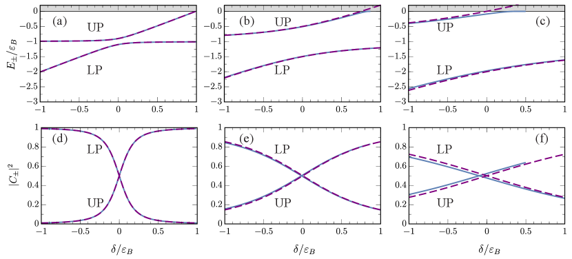
Figure 1 shows the polariton energies and the corresponding photon and exciton fractions according to Eqs. (12) and (16). We find that they agree extremely well with the results of treating the excitons and photons as two coupled oscillators [31], even when the Rabi coupling is comparable to the exciton binding energy as in structures containing multiple GaAs quantum wells. In particular, our scheme provides an improved agreement between the two models than that obtained in Ref. [23], which considered a similar electron-hole-photon model. Moreover, our scheme is technically simpler to implement since Eqs. (12)-(17) are fully analytic and do not require the introduction of an additional infrared cutoff. We now proceed to derive these results.
II.2.1 Renormalization procedure
The central idea of the renormalization procedure is to relate the parameters in Eq. (11) to the experimental observables in the coupled-oscillator model of excitons and photons. At a technical level, we note that our renormalization of the electron-hole-photon model is conceptually similar to that of atoms interacting via both an open and a closed channel in three dimensions [32]. First, let us consider the case of small exciton-photon Rabi coupling such that the polariton energy is close to the exciton energy, i.e., with the energy correction. In the limit , the electron-hole part of the polariton wave function in Eq. (14) can then be approximated as proportional to the exciton wave function in Eq. (5), , where is a complex number. Within this approximation, we use the exciton Schrödinger equation in Eq. (4) to find that Eq. (11) takes the form:
| (18a) | ||||
| (18b) | ||||
Written in matrix form we have
| (19) |
where we have identified the off-diagonal term as the experimentally measurable Rabi coupling introduced in Eq. (13). Evaluating the sum using Eqs. (5) and (7) allows us to relate the bare coupling to and the exciton parameters,
| (20) |
Since diverges logarithmically with the cutoff in Eq. (7), we thus require to ensure that is finite in our renormalization scheme.
Equation (19) yields the spectrum of two coupled oscillators:
| (21) |
where is the (bare) photon-exciton detuning. Thus we see that in the limit of small Rabi coupling we recover the usual spectrum [1, 2] of the lower and upper polaritons. We also note that the photon and exciton fractions can be written as
| (22a) | ||||
| (22b) | ||||
Note the similarity to our exact equation (16). In particular, the coefficients exactly match in the limit where the polariton energies approach the exciton energy.
In general, the exciton wave function will be modified by the coupling to light, unlike what we have assumed in the above analysis. We therefore now proceed to find the exact spectrum of Eq. (11), which also allows us to arrive at the modified Hopfield coefficients. To this end, we define which is finite as since and . Equation (11) then becomes
| (23a) | ||||
| (23b) | ||||
Rearranging Eq. (23a) and then inserting (23b), we find
| (24) |
where, in the last line, we have used Eq. (20) and the fact that as . Replacing on the left hand side using Eq. (7), we finally obtain Eq. (12) for the polariton spectrum:
| (25) |
The solutions to Eq. (25) correspond to the exact polariton energies for the Hamiltonian (II), under the assumption that (which is always true for the lower polariton). Expanding the logarithm to leading order around allows us to recover the spectrum of two coupled oscillators in Eq. (21).
II.2.2 Effective photon-exciton detuning
As noted above, the coupling of the photon to the active semiconductor medium can also shift the cavity photon frequency. In experiment, the Rabi coupling and the exciton-photon detuning are parameters that are fitted from the observed polariton spectrum. Therefore, we now define an effective detuning that would result from such a fitting procedure. This allows us to directly relate the bare photon frequency to a detuning . In contrast to the case of Coulomb interactions [24], we find that the shift is independent of the cutoff for the contact-interaction model.
To capture the leading order correction to the cavity frequency when , we take with small compared to , and then insert this into Eq. (12):
| (27) |
Using the lowest-order expressions for the polariton energies, Eq. (21), and keeping terms only up to order and , we find
| (28) |
This leads to the expression in Eq. (17). As seen in Fig. 1, with this definition we have an excellent agreement with the coupled oscillators model up to Rabi couplings , well beyond our initial assumption that . In particular, had we instead used the bare detuning , our results would be shifted by in panels (c) and (f), and hence the definition (17) substantially improves the agreement with the coupled-oscillator model.
II.3 Diagrammatic formulation
In this section, we provide an alternative description of exciton-polaritons using a diagrammatic formulation. While this is equivalent to the operator approach described above, the advantage of the diagrammatic formulation is that it allows a straightforward characterization of repeated scattering processes. As we shall see, this enables us to obtain the polariton propagator in closed form, and it provides a convenient starting point for further few-body studies such as the polariton-electron scattering discussed in Sections III and IV.
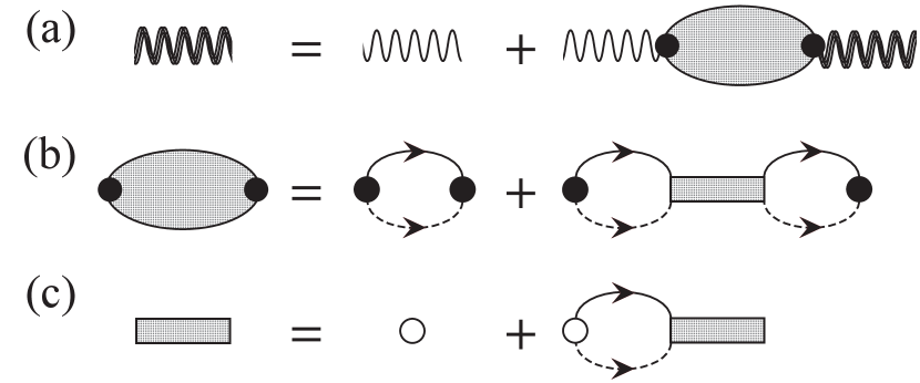
We start by considering the properties of a photon interacting with an undoped 2D semiconductor in a microcavity. The microcavity photon will be modified by repeated interactions with electron-hole pairs, which includes both bound excitons and unbound electron-hole pairs in the continuum. Referring to Fig. 2, the resulting “dressed” photon is characterized by the self-energy [33]. Following Ref. [24], we obtain the dressed photon propagator from the Dyson equation in Fig. 2(a):
| (29) |
where and are, respectively, the energy and momentum of the photon. In the absence of the active medium, we have the bare photon propagator
| (30) |
where the imaginary infinitesimal shifts the poles into the lower half of the complex plane and ensures that the photon propagates forward in time. Note that we can also incorporate the decay of photons from the microcavity by setting the imaginary part equal to the decay rate. However, we neglect this decay rate since it is much smaller than the Rabi coupling in the regime of strong light-matter coupling, and it therefore only has a negligible effect on the scattering. In other words, we consider a closed quantum system. In the following, we will always implicitly assume that the energy carries an infinitesimal positive imaginary part, that is, we will be working with retarded Green’s functions.
As shown in Fig. 2(b), the photon self-energy consists of two terms: , with the exciton kinetic energy and the exciton mass. These contain all possible processes that involve the excitation of an electron-hole pair, and they thus only depend on the energy in the exciton center-of-mass frame. Hence, the dependence simply appears as a shift in the energy.
Within the model (II), we have
| (31a) | ||||
| (31b) | ||||
where is the polarization bubble diagram corresponding to an electron-hole pair. Since and the bare coupling , the term vanishes when the momentum cutoff . On the other hand, we have from Eq. (20) and the fact that as .
The electron-hole matrix (or exciton propagator) is shown in Fig. 2(c), and corresponds to
| (32) |
We can renormalize the bare using Eq. (7) to finally obtain the standard expression in Eq. (8), see Appendix B.
Combining all of these expressions yields the explicit form for the dressed photon propagator:
| (33) |
where can be related to the physical photon-exciton detuning via Eq. (17). To simplify the notation, we have not explicitly written the imaginary infinitesimal on the energy. The poles of the photon propagator contain information about the entire polariton spectrum. Specifically, the denominator of Eq. (33) is zero when we have
| (34) |
Indeed, for , this exactly corresponds to Eq. (25) from the operator approach. For general , we denote the polariton energy solutions of Eq. (34) as .
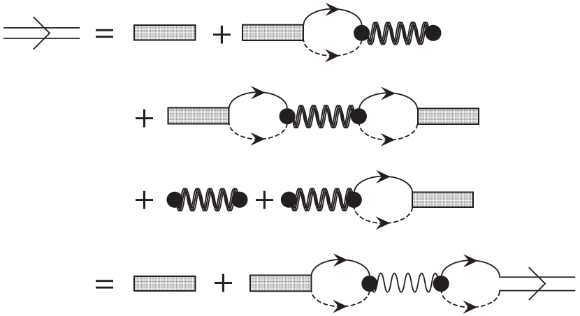
In addition to the dressed photon propagator, we have what we call the “polariton propagator” shown in Fig. 3, which instead focuses on the behavior of the matter component of the polariton. Like the dressed photon, it contains all the possible scattering processes involving an electron-hole pair or photon. In the absence of light-matter coupling, it reduces to , the electron-hole matrix at center-of-mass momentum . Suppressing the dependence on energy and momentum, Fig. 3 reads:
| (35) |
Here, we again use and to remove terms that vanish in the limit , while in the last line, we use the relation . Thus, the polariton propagator finally reads:
| (36) |
It is also straightforward to show that the polariton and photon propagators are related via
| (37) |
The polariton propagator has precisely the same poles as the dressed photon propagator in Eq. (33). However, the poles of the photon propagator have residues corresponding to the photon fractions of the polaritons:
| (38) |
while the residues for the poles of the polariton propagator instead correspond to the matter component,
| (39) |
with the electron-hole normalization factors
| (40) |
At , the Hopfield coefficients and the normalization factors reduce to the corresponding expressions in Eqs. (16) and (15).
III Polariton-electron interactions in the Born approximation
Due to the complexity of the Coulomb interaction, an exact solution of few-body scattering processes such as polariton-electron and polariton-polariton scattering in strongly coupled light matter systems remains elusive. Instead, the interactions are typically approximated by considering their corresponding excitonic counterparts multiplied by appropriate powers of the excitonic Hopfield coefficient:
| (41) |
where is the polariton-electron (exciton-electron) interaction constant, while is the polariton-polariton (exciton-exciton) interaction constant. Note that we have specialized to the lower polariton here, but similar expressions are used for the upper polariton with the simple replacement . The standard approach is to calculate the interaction strengths within the Born approximation [11, 12, 13, 14], with effects due to very strong light-matter coupling included via the calculation of additional matrix elements [11, 16, 17, 18, 19]. The polariton-polariton interaction strength has also been calculated in -matrix approaches that treat the exciton as an inert object, first focusing on the case of cross-circularly polarized polaritons [34] and recently for both the singlet and triplet scattering configurations in multilayer systems [35].
In this paper, we provide the first exact microscopic calculation of polariton-electron scattering, within a simplified model of contact interactions between charges. It is therefore imperative to compare our results with the standard Born approximation. Therefore, in this section we will describe the results of the Born approximation within our model. We will furthermore argue that the Born approximation provides a strict upper bound on the interaction energy shift (in the limit of zero momentum) when there are no lower-lying bound states.
III.1 Operator approach
The analytic expression for the polariton wave function obtained in the previous section (see also the finite-momentum generalization in Appendix A) allows us to straightforwardly evaluate the Born approximation for polariton-electron scattering. For simplicity, we consider the frame where the center-of-mass momentum is zero, since in that case the different partial wave components of the scattering separate. Since the electron has a relatively flat dispersion, our results are likely to be insensitive to the actual electron momentum and will thus be dominated by the polariton momentum.
The Born approximation consists in approximating the scattering matrix by the first term in the Born series, which corresponds to evaluating the matrix element of the polariton-electron interaction potential. Taking the incoming (outgoing) polariton and electron to have momenta (), this matrix element takes the form
| (42) |
where the operator creates a polariton with momentum , see Eq. (58) in Appendix A. We assume energy and momentum conservation such that the scattering is elastic, i.e., we take . Here, the subtraction of the energy of the non-interacting particles from the Hamiltonian, Eq. (II), ensures that we only evaluate the polariton-electron interaction potential. Using the exact polariton wave function from Appendix A, we find
| (43) |
where the sign in the middle line arises from the exchange of identical fermions. As anticipated, we see that the exciton fraction naturally emerges from the normalization of the polariton wave function.
In Fig. 4 we illustrate the Born approximation for elastic polariton-electron scattering. The exciton fraction quickly increases at low momentum, which dominates the behavior at momenta up to the polariton dispersion inflection point above which the exciton fraction is very close to unity. Apart from the Hopfield coefficient , there is also a momentum and angular dependence through the kinetic energies and the wave function normalization; however we find that this dependence is generally quite weak. Above the inflection point, it leads to a slow decline for increasing momentum.
Specializing to zero momentum, we may define a low-energy polariton-electron interaction constant , which takes the form
| (44) |
This is precisely the exciton fraction multiplied by the exciton-electron interaction, . Note that this is quite close to the corresponding result obtained in the case of Coulomb electronic interactions [37]: Using the formalism developed in Ref. [24], we find . We emphasize that the polariton-electron Born approximation in Eq. (44) only depends on the light-matter coupling through the exciton fraction, while it is independent of the absolute strength of the light-matter coupling, .
III.2 Diagrammatic approach
The polariton-electron scattering process can also be calculated diagrammatically, as shown in Fig. 5. In this case, the Born approximation corresponds to the first diagram on the right hand side, which involves the exchange of a hole with momentum [38]. This gives
| (45) |
where the minus sign is a consequence of fermionic statistics and
| (46) |
is the free hole Green’s function. Each external polariton line in the diagram contributes the square root of the residue of the propagator at the pole, and the normalization of the incoming and outgoing lines is the same since . The residue is precisely — see Eq. (39). Using the definition of the hole propagator, and comparing Eq. (III.1) with Eq. (III.2) we thus see that the Born approximation within the two approaches coincides, as it should.
III.3 Upper bound on the interaction energy shift
We now argue that the Born approximation is conceptually important since it provides an upper bound on the polariton-electron interaction constant . We start by noting that the ground-state energy for an electron and a lower polariton in an area can be written as
| (47) |
where is the exact interacting polariton-electron state. Here we have assumed that there are no lower-energy polariton-electron bound states so that consists of the non-interacting kinetic energy plus a two-body interaction term. We momentarily keep the area explicit so that we can keep track of powers of . In particular, note that , where the last term arises from the composite nature of the polariton.
Rearranging Eq. (47) and keeping only terms up to order then gives
| (48) |
where the second line follows from the fact that the non-interacting state can be viewed as a variational approximation to the exact interacting state . Thus, we finally arrive at
| (49) |
Hence, the Born approximation serves as a strict upper bound on the interaction energy shift. This observation is quite general and is independent of the details of the underlying interactions, e.g., it also applies to polariton-polariton scattering and to more realistic interactions between charged particles. The only requirement is that there are no lower energy bound states (such as trions) and that the Hamiltonian faithfully reproduces the low-energy physics. Therefore, any diverging interaction strength obtained in the absence of a bound state must be an artefact of the approximation [35].
IV Polariton-electron interactions
We now present our full diagrammatic calculation of the polariton-electron interaction strength, which is exact within the Hamiltonian (II). Our approach follows similar calculations originally introduced in the context of neutron-deuteron scattering by Skorniakov and Ter-Martirosian [39], and later applied to cold atomic gases [40, 41, 42, 43]. Subsequently, the theory of the effective three-body problem at finite momentum was developed in a series of papers [44, 45, 46, 47], and this has already been successfully applied to describe the strong atom-dimer attraction observed in mass-imbalanced ultracold Fermi gases [48].
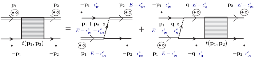
The exact scattering of an electron and a polariton can be represented as an infinite sum of terms where the two electrons involved in the process exchange a hole, and the Born approximation corresponds to keeping only the first term in this series. While it is not possible to simply calculate each term in this sum separately and then sum them up, the key observation that enables an exact solution of the polariton-electron scattering is that the sum satisfies an integral equation as illustrated in Fig. 5. Indeed, iterating the right hand side of this equation generates all possible terms where the electrons exchange a hole. Diagrammatically, the equation for the polariton-electron matrix takes the exact same form as the exciton-electron matrix, the only difference being the replacement of the exciton with the polariton propagator, and the associated change in dispersion.
To compute the matrix, we take the incoming and outgoing electrons to have momentum and and energy and , respectively, while the polaritons have momenta and and energies and , respectively, with the total collision energy. The equation for the (unnormalized) polariton-electron matrix illustrated in Fig. 5 takes the explicit form [44, 47]
| (50) |
where the minus signs on the right hand side follows from the exchange of identical electrons 333Note that the electron propagator in the last term in Fig. 5 has a simple pole in the upper half of the complex plane, while all other propagators have their non-analytic structure only in the lower half plane. This allows us to perform the integral over by closing the contour in the upper half plane, effectively removing that propagator and setting the electron dispersion to its on-shell value in the other propagators. For more details, see, e.g., Ref. [41].. We see that this is an integral equation in the first momentum index of , and we can therefore only set at the end of calculation. In order to have on-shell scattering, we take the total energy to be . The normalization is the same as in Eq. (III.2), and therefore the normalized and on-shell matrix takes the form
| (51) |
This quantifies the strength of scattering between electrons and polaritons.
IV.1 Scattering of slow particles
It is of particular interest to consider the scattering of polaritons at vanishing momentum due to the realization of polariton Bose-Einstein condensation [26]. First, it is important to clarify precisely what we mean by this limit. It is well-known [25, 28] that the scattering matrix of 2D quantum particles with short range interactions (such as the exciton-electron interaction between a charge and an induced dipole) must approach zero as the collision energy vanishes. However, in the case of polariton-electron scattering, this only becomes relevant for exceedingly small momenta below those where the typical scale of exciton-electron scattering is comparable to [35]. Because of the very small photon mass, this momentum scale corresponds to a length scale much larger than the size of the universe, and this effect can therefore be discarded. Thus, we can safely take the limit in our numerical solutions, since we will never encounter such an extreme scale. We emphasize that this is a dramatic consequence of the lack of Galilean invariance in the polariton system due to the strong coupling of excitons and photons.
For scattering at small momenta, we set and in Eq. (50) and perform the integration over the angle between and assuming . The remaining integral equation is then solved using Gauss-Legendre quadrature; for more details, see Appendix C. As a result, we obtain the exact polariton-electron interaction constant
| (52) |
where we use the same normalization as in Eq. (51). Note the similarities between this expression and that in Eq. (44) within the Born approximation.
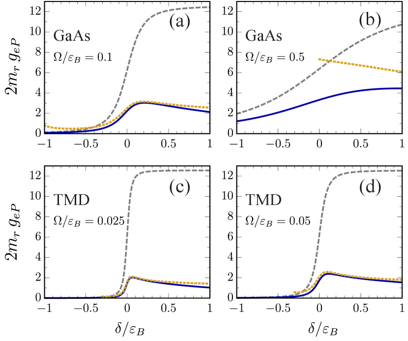
Figure 6 shows a comparison of the polariton-electron interaction constant obtained from different methods for parameters relevant to both TMDs and GaAs quantum wells. The exact diagrammatic calculation, , can be used as a standard to gauge the correctness of other calculations. We see that generally the interaction strength increases as the polariton goes from being photonic at negative detuning to more excitonic at positive detuning, in agreement with the expectation from the Born approximation, Eq. (44). However, we find that the exact calculation features a peak at small positive detuning when the ratio is not too large, which is a qualitative feature that is missed by the Born approximation. Furthermore, the Born approximation generically overestimates the interaction strength, and this effect is most dramatic for relatively small values of the ratio such as in TMDs. For larger , the exact result approaches and thus we expect the Born approximation to be more accurate for GaAs quantum wells, which is consistent with recent measurements of the polariton-polariton interaction strength [57]. Note that applies to the case of multiple GaAs quantum wells and thus a full description requires us to take account of the non-trivial effects of multiple layers [35].
We can understand these results by noting that at momenta above the inflection point, the polariton propagator in Eq. (36) quickly approaches the exciton propagator, , in Eq. (8). Taking the limit , we observe that Eq. (50) has the exact same functional form as in exciton-electron scattering [47], the only difference being the change in collision energy due to the light-matter coupling. This motivates the interpretation of polariton-electron scattering as an off-shell exciton-electron scattering process, similarly to recent results on polariton-polariton interactions [35]. To make this explicit, we consider the universal form of the low-energy exciton-electron scattering matrix
| (53) |
where we define as the reduced exciton-electron mass. Unlike the light-matter coupled system, the exciton-electron scattering only depends on the collision energy, since the exciton-electron system is Galilean invariant. Equation (53) is valid at collision energies , where the energy scale depends on the precise details of the electronic interactions and on the electron-hole mass ratio 444In general, there are finite range corrections to Eq. (53), which add a term in the denominator [28]. In the absence of other scales, the effective range and therefore such terms are not important when .. We thus estimate the polariton-electron scattering in the limit of low momentum by the off-shell exciton-electron expression
| (54) |
which is valid when .
Equation (54) yields the yellow dashed line in Fig. 6, which is seen to closely follow the exact polariton-electron scattering result for sufficiently low Rabi coupling, reproducing all qualitative features. In particular, it works exceptionally well in the case of TMD monolayers, which supports the approximation for polariton-polariton interactions introduced in Ref. [35]. Note that Eq. (54) predicts a resonance when the (negative) collision energy is comparable to , such as in GaAs with a very large Rabi coupling in panel (b). However, this resonance is spurious and can be cured by including higher order terms in the phase shift, and it is also absent in our exact calculation.
While Eq. (54) is conceptually similar to the Born approximation, Eq. (44), we see that the fact that the exciton-electron scattering should be considered off-shell leads to a qualitative difference in the behavior as a function of detuning. We stress that there is no a priori reason why this conclusion should not generalize beyond contact electronic interactions to Coulomb or Keldysh [59] type potentials in, e.g., GaAs or TMDs: At large electron-exciton separation , both of these electronic potentials will result in an effective exciton-electron potential that decays like corresponding to the interaction between a charge and an induced dipole. Such a potential qualifies as short ranged [27], and therefore the low-energy exciton-electron scattering necessarily follows the form in Eq. (53). Furthermore, this approximation relies only on a single quantity, the low-energy scale , which can be fitted in experiment or calculated in exact solutions of the exciton-electron three-body problem such as in the recent work by Fey et al. [60]. Finally, we note that since only appears under a logarithm, our results are not very sensitive to realistic variations in this parameter, and they may therefore be expected to be quite accurate even at a quantitative level.
IV.2 Polariton-electron interactions at finite momentum
We now turn to the interaction of an electron and a polariton at finite momentum which, as we shall show, can be strongly enhanced compared with their exciton-electron counterpart. As previously noted, we will restrict our attention to the case of zero center-of-mass momentum, which allows us to perform a partial wave decomposition of the matrix as follows [25]:
| (55) |
where is the angular momentum quantum number and is the angle between and . Obviously, the scattering in the limit of zero momentum discussed in the previous subsection corresponds to -wave, . This decomposition allows us to solve the integral equation as a function of a single parameter, the magnitude of the incident relative momentum. The main challenge then is that the electron-hole matrix in Eq. (50) has a simple pole when [44], and we discuss how to deal with this in Appendix C. Once we have solved for the partial wave amplitudes , we obtain the normalized scattering matrix in the ’th partial wave via
| (56) |
similarly to Eq. (51). In this work, we focus on -wave scattering, which we denote by . However, we note that higher partial waves (in particular -wave) can become important in the scattering of polaritons with heavy holes [45, 47] due to the presence of hole-hole-electron trion bound states which have previously been discussed in the context of quantum wells [61] and TMD monolayers [62, 63] or strongly screened electronic interactions [64, 51].
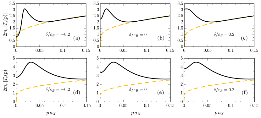
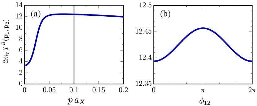
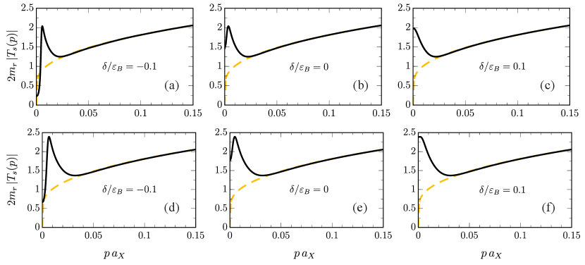
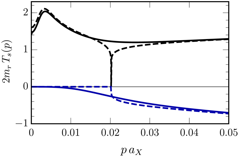
Figures 7 and 8 show our results for the polariton-electron scattering at finite relative momentum for the case of a TMD monolayer and for a GaAs quantum well, respectively. A striking aspect of our results is the presence of a resonance-like peak at momenta close to the polariton inflection point. The peak is most pronounced for zero and negative detuning and it is enhanced with increased Rabi coupling. By contrast, we find that the peak is completely absent in the case of exciton-electron scattering (also shown in the figures), where we obtain the corresponding matrix using Eq. (53) at collision energy . At a qualitative level, the results for GaAs and a TMD monolayer embedded in a microcavity are similar, although the generally larger ratios of Rabi coupling to exciton binding energy in GaAs means that the relative enhancement of interactions in GaAs microcavity is larger. For relative momenta above the polariton inflection point, we see that the polariton-electron matrix quickly reduces to the exciton-electron matrix, as we would expect since in that limit the exciton fraction approaches unity.
As in the case of scattering at low momenta, we can understand the resonance-like feature in the polariton-electron scattering at finite momentum in terms of off-shell exciton-electron scattering. Using a similar reasoning to that which led to Eq. (54), we approximate
| (57) |
We illustrate this in Fig. 9 for the case of the TMDs with a smaller ratio of Rabi coupling to exciton binding energy (MoSe2, WSe2, or MoS2). We see that this approximation works extremely well for almost all momenta, the only difference being a narrow region around the momentum where the collision energy vanishes. By analyzing the two contributions in Eq. (57), we conclude that the resonance-like feature is due to a competition between the exciton fraction — which quickly approaches unity when the momentum approaches the polariton inflection point — and the fact that scattering is suppressed when the collision energy approaches zero. Figure 9 also shows that the polariton-electron matrix is nearly purely real at the peak, which we can also understand from Eq. (57) since exciton-electron scattering only features an imaginary part for positive collision energy.
Crucially, our results in Figures 7-9 imply that the polariton-electron matrix is essentially never smaller than that of an electron and an exciton at a given momentum, the only exception being at a very large negative detuning. This is in spite of the suppression due to the reduced exciton fraction in the polariton, and it demonstrates that the strong energy shift of the scattering process due to the light-matter coupling is the dominant effect. Our result can thus be understood as an effective photon-mediated enhancement of exciton-electron scattering, which is a major qualitative difference compared with the commonly applied assumption in the Born approximation, Eq. (41). As we have derived this effect in a fully microscopic model, and since it agrees with the universal low-energy behavior, Eq. (57), we expect that this conclusion carries over to more realistic interactions between charged particles.
Given the general nature of our arguments, the enhancement of interactions between polaritons and electrons is also expected to carry over to other geometries, such as systems where a 2D electron gas is in proximity to a 2D exciton-polariton condensate. Here, it would be interesting to investigate whether the enhanced interactions could lead to stronger drag effects [65], or to more robust superconductivity [66, 67].
V Conclusions and outlook
We have presented a microscopic approach to exciton-polaritons in a 2D semiconductor embedded in a microcavity. By treating the semiconductor interactions as strongly screened, we have found an analytic expression for the polariton propagator, which serves as a starting point for further few- and many-body calculations. We have applied our microscopic description of polaritons to the calculation of the scattering of electrons and polaritons in a manner that is exact within our approximation. Remarkably, we have shown that polariton-electron scattering is nearly always stronger than exciton-electron scattering at a given momentum, in contrast to the prevailing belief based on the Born approximation. In particular, we have shown that the interactions can be strongly enhanced up to and beyond the inflection point of the polariton dispersion, giving rise to a resonance-like feature. While this qualitatively new and unexpected behavior may appear counter-intuitive, we have argued that the enhancement of scattering is due to the strong light-matter coupling that shifts the collision energy compared with exciton-electron scattering, and hence this is a generic effect which is independent of our approximation of screened interactions.
Our approach can be directly applied to a large class of other few-body problems in light-matter coupled systems. Of particular interest is the case of spin-polarized electrons interacting with an exciton-polariton of opposite circular polarization. In this case, the exciton-electron system features a trion bound state which leads to resonantly enhanced interactions, and this has recently enabled the observation of polaron-polaritons [68, 69]. Furthermore, using the four-body techniques developed in the context of cold atomic gases Refs. [70, 71, 41, 42], our approach can be straightforwardly generalized to the calculation of polariton-polariton and polariton-exciton interactions. This would, for instance, allow a fully microscopic description of the scattering resonances due to coupling to a biexciton bound state, as observed in Refs. [9, 72, 73] and also analyzed in Refs. [74, 75]. Finally, the microscopic theory of exciton-polaritons for the case of Coulomb interactions developed in Ref. [24] also allows a natural diagrammatic representation, which can be applied to few-body scattering problems. Hence our approach holds promise as a fully microscopic theory in which to obtain key quantities in exciton-polariton systems.
Acknowledgements.
We thank Olivier Bleu, Dmitry Efimkin, Eliezer Estrecho, Emma Laird, David Neilson, Elena Ostrovskaya, and Maciej Pieczarka for useful discussions, and we acknowledge support from the Australian Research Council Centre of Excellence in Future Low-Energy Electronics Technologies (CE170100039). JL is furthermore supported through the Australian Research Council Future Fellowship FT160100244.Appendix A Polariton at finite momentum
In this Appendix, we apply the operator approach discussed in Sec. II.2 to a polariton at finite momentum . The polariton creation operator is defined as:
| (58) |
where with the exciton mass. The Schrödinger equation can be obtained by projecting onto the electron-hole and photon parts of Eq. (58), which gives:
| (59a) | ||||
| (59b) | ||||
The momentum serves as an external parameter in Eq. (59) and thus the renormalization procedure is the same as in Sec. II.2, as we now demonstrate.
We first consider the case of small exciton-photon Rabi coupling where the polariton energy is close to the exciton energy, i.e., . In the limit , the electron-hole part of the polariton wave function can be approximated as proportional to the exciton wave function, , where is a complex number. Within this approximation, Eq. (59) takes the form:
| (60a) | ||||
| (60b) | ||||
Written in matrix form we have
| (61) |
where we have identified the off-diagonal term as the experimentally measurable Rabi coupling introduced in Eq. (13). Equation (61) yields the spectrum of two coupled oscillators as
| (62) |
with the Hopfield coefficients
| (63a) | ||||
| (63b) | ||||
After the renormalization, we follow a similar derivation as that carried out in Eqs. (23) and (24) to find that the exact polariton dispersion satisfies
| (64) |
With the polariton dispersion established, we can return to Eq. (59) to solve for the electron-hole wave function. Since the right hand side of Eq. (59a) is independent of , we immediately know that the electron-hole wave function has the same functional form as in Eq. (14):
| (65) |
with
| (66) |
We can also extract the Hopfield coefficients in Eq. (16) in the same manner as in Sec. II.2. This straightforwardly yields the same expressions as in the diagrammatic section II.3, and allows us to obtain an analytic expression for the electron-hole wave function in terms of experimentally measurable parameters.
Appendix B Electron-hole T matrix
In this Appendix, we derive the expression for the exciton propagator, Eq. (8). Starting from the electron-hole matrix diagram shown in Fig. 2(c), the exciton propagator at zero momentum reads:
| (67) |
where has been related to an integral by Eq. (7),
| (68) |
The bubble integral in Eq. (67) can be worked out explicitly:
| (69) |
where we can take the limit in the difference in the second line, since this is ultraviolet convergent, while the last sum diverges as when . Inserting Eqs. (69) and (68) into Eq. (67) we obtain the expression for :
| (70) |
Appendix C Partial wave decomposition and numerical solution of the polariton-electron scattering integral equation
We now outline how we numerically investigate the key equation of polariton-electron scattering, namely Eq. (50), which we rewrite here in integral form by taking the continuum limit
| (71) |
where we again take the total energy . This represents an integral equation in the first momentum of the function , while it only depends parametrically on the second. There are two main challenges to deal with when solving this equation. First, the integral equation depends on the angle between incident and outgoing relative momenta. This angular dependence increases the numerical complexity, which we resolve by performing a partial wave decomposition. Second, the polariton propagator has a simple pole, which we address by using a principal value prescription.
Let us first discuss the partial wave decomposition. As in Eq. (55), we define
| (72) |
with the angle between and . This can be inverted to find
| (73) |
Similarly, we define the partial wave decomposition of the hole Green’s function
| (74) |
and
| (75) |
Now let us define the angles of the vectors , , and in Eq. (71) as , , , respectively. Then we can take in the integral, while the angle between and is with . Inserting the expansions (72) and (74) in Eq. (71) and focussing only on the angular integral, we have
| (76) |
where and are the partial wave quantum numbers of the hole propagator and the polariton-electron matrix inside the integral, respectively. We see that this only depends on the angle which is the same that we have on the left hand side of Eq. (71). Therefore, applying the operator to the equation, we find that we must have , and we arrive at the equation
| (77) |
The polariton propagator in Eq. (77) has a simple pole at , since by definition diverges as . To circumvent this pole, we use the fact that
| (78) |
where denotes the principal part. Using this in Eq. (77), we find
| (79) |
where
| (80) | ||||
| (81) |
The prefactor in the first term of Eq. (79) is independent of and depends only on . Since the multiplication by a constant prefactor in the inhomogenous term of an integral equation does not change its structure, we can instead solve the auxilliary equation
| (82) |
where the pole is explicitly excluded using the principal value prescription [44]. We then relate the on-shell unnormalized matrix to via
| (83) |
or, in other words,
| (84) |
We solve Eq. (82) using Gauss-Legendre quadrature.
In the case of scattering at low momentum, we can further simplify the problem, since the simple pole in this case disappears. We then set and in Eq. (77), which can then be written as
| (85) |
References
- Deng et al. [2010] H. Deng, H. Haug, and Y. Yamamoto, Exciton-polariton Bose-Einstein condensation, Rev. Mod. Phys. 82, 1489 (2010).
- Carusotto and Ciuti [2013] I. Carusotto and C. Ciuti, Quantum fluids of light, Rev. Mod. Phys. 85, 299 (2013).
- Byrnes et al. [2014] T. Byrnes, N. Y. Kim, and Y. Yamamoto, Exciton-polariton condensates, Nat. Phys. 10, 803 (2014).
- Amo et al. [2009] A. Amo, J. Lefrère, S. Pigeon, C. Adrados, C. Ciuti, I. Carusotto, R. Houdré, E. Giacobino, and A. Bramati, Superfluidity of polaritons in semiconductor microcavities, Nature Physics 5, 805 (2009).
- Sanvitto et al. [2010] D. Sanvitto, F. M. Marchetti, M. H. Szymańska, G. Tosi, M. Baudisch, F. P. Laussy, D. N. Krizhanovskii, M. S. Skolnick, L. Marrucci, A. Lemaître, J. Bloch, C. Tejedor, and L. Viña, Persistent currents and quantized vortices in a polariton superfluid, Nature Physics 6, 527 (2010).
- Amo et al. [2010] A. Amo, T. C. H. Liew, C. Adrados, R. Houdré, E. Giacobino, A. V. Kavokin, and A. Bramati, Exciton-polariton spin switches, Nature Photonics 4, 361 (2010).
- Muñoz-Matutano et al. [2019] G. Muñoz-Matutano, A. Wood, M. Johnsson, X. Vidal, B. Q. Baragiola, A. Reinhard, A. Lemaître, J. Bloch, A. Amo, G. Nogues, B. Besga, M. Richard, and T. Volz, Emergence of quantum correlations from interacting fibre-cavity polaritons, Nature Materials 18, 213 (2019).
- Delteil et al. [2019] A. Delteil, T. Fink, A. Schade, S. Höfling, C. Schneider, and A. İmamoğlu, Towards polariton blockade of confined exciton–polaritons, Nature Materials 18, 219 (2019).
- Takemura et al. [2014] N. Takemura, S. Trebaol, M. Wouters, M. T. Portella-Oberli, and B. Deveaud, Polaritonic Feshbach resonance, Nature Physics 10, 500 (2014).
- Tan et al. [2020] L. B. Tan, O. Cotlet, A. Bergschneider, R. Schmidt, P. Back, Y. Shimazaki, M. Kroner, and A. İmamoğlu, Interacting Polaron-Polaritons, Phys. Rev. X 10, 021011 (2020).
- Tassone and Yamamoto [1999] F. Tassone and Y. Yamamoto, Exciton-exciton scattering dynamics in a semiconductor microcavity and stimulated scattering into polaritons, Phys. Rev. B 59, 10830 (1999).
- Ramon et al. [2002] G. Ramon, R. Rapaport, A. Qarry, E. Cohen, A. Mann, A. Ron, and L. N. Pfeiffer, Scattering of polaritons by a two-dimensional electron gas in a semiconductor microcavity, Phys. Rev. B 65, 085323 (2002).
- Malpuech et al. [2002] G. Malpuech, A. Kavokin, A. Di Carlo, and J. J. Baumberg, Polariton lasing by exciton-electron scattering in semiconductor microcavities, Phys. Rev. B 65, 153310 (2002).
- Hartwell and Snoke [2010] V. E. Hartwell and D. W. Snoke, Numerical simulations of the polariton kinetic energy distribution in GaAs quantum-well microcavity structures, Phys. Rev. B 82, 075307 (2010).
- Shahnazaryan et al. [2017] V. Shahnazaryan, I. Iorsh, I. A. Shelykh, and O. Kyriienko, Exciton-exciton interaction in transition-metal dichalcogenide monolayers, Phys. Rev. B 96, 115409 (2017).
- Rochat et al. [2000] G. Rochat, C. Ciuti, V. Savona, C. Piermarocchi, A. Quattropani, and P. Schwendimann, Excitonic Bloch equations for a two-dimensional system of interacting excitons, Phys. Rev. B 61, 13856 (2000).
- Combescot et al. [2007] M. Combescot, M. A. Dupertuis, and O. Betbeder-Matibet, Polariton-polariton scattering: Exact results through a novel approach, Europhysics Letters (EPL) 79, 17001 (2007).
- Combescot et al. [2008] M. Combescot, O. Betbeder-Matibet, and F. Dubin, The many-body physics of composite bosons, Physics Reports 463, 215 (2008).
- Glazov et al. [2009] M. M. Glazov, H. Ouerdane, L. Pilozzi, G. Malpuech, A. V. Kavokin, and A. D’Andrea, Polariton-polariton scattering in microcavities: A microscopic theory, Phys. Rev. B 80, 155306 (2009).
- Li et al. [2020] G. Li, O. Bleu, M. M. Parish, and J. Levinsen, Enhanced scattering between electrons and exciton-polaritons in a microcavity (2020), arXiv:2008.09281 .
- Yamaguchi et al. [2012] M. Yamaguchi, K. Kamide, T. Ogawa, and Y. Yamamoto, BEC–BCS-laser crossover in Coulomb-correlated electron–hole–photon systems, New Journal of Physics 14, 065001 (2012).
- Hanai et al. [2017] R. Hanai, P. B. Littlewood, and Y. Ohashi, Dynamical instability of a driven-dissipative electron-hole condensate in the BCS-BEC crossover region, Phys. Rev. B 96, 125206 (2017).
- Hu and Liu [2020] H. Hu and X.-J. Liu, Quantum fluctuations in a strongly interacting Bardeen-Cooper-Schrieffer polariton condensate at thermal equilibrium, Phys. Rev. A 101, 011602 (2020).
- Levinsen et al. [2019a] J. Levinsen, G. Li, and M. M. Parish, Microscopic description of exciton-polaritons in microcavities, Phys. Rev. Research 1, 033120 (2019a).
- Adhikari [1986] S. K. Adhikari, Quantum scattering in two dimensions, American Journal of Physics 54, 362 (1986).
- Kasprzak et al. [2006] J. Kasprzak, M. Richard, S. Kundermann, A. Baas, P. Jeambrun, J. M. J. Keeling, F. M. Marchetti, M. H. Szymańska, R. André, J. L. Staehli, V. Savona, P. B. Littlewood, B. Deveaud, and L. S. Dang, Bose–Einstein condensation of exciton polaritons, Nature 443, 409 (2006).
- Landau and Lifshitz [2013] L. D. Landau and E. M. Lifshitz, Quantum mechanics: non-relativistic theory, Vol. 3 (Elsevier, 2013).
- Levinsen and Parish [2015] J. Levinsen and M. M. Parish, Strongly interacting two-dimensional Fermi gases, Annu. Rev. Cold Atoms Mol. 3, 1 (2015).
- Note [1] If and/or , the upper polariton enters the continuum of unbound electron-hole states. In that case, one must analytically continue the energy slightly into the complex plane, .
- Note [2] The variational approach developed by Khurgin [76] approximated the functional form of the electron-hole wave function as unchanged in the presence of light-matter coupling. While this is an approximation in the Coulomb case studied in that work [24], we see that it is exact for strongly screened electron-hole interactions.
- Hopfield [1958] J. J. Hopfield, Theory of the Contribution of Excitons to the Complex Dielectric Constant of Crystals, Phys. Rev. 112, 1555 (1958).
- Werner et al. [2009] F. Werner, L. Tarruell, and Y. Castin, Number of closed-channel molecules in the BEC-BCS crossover, The European Physical Journal B 68, 401 (2009).
- Fetter and Walecka [2003] A. L. Fetter and J. D. Walecka, Quantum Theory of Many-Particle Systems (Dover, New York, USA, 2003).
- Wouters [2007] M. Wouters, Resonant polariton-polariton scattering in semiconductor microcavities, Phys. Rev. B 76, 045319 (2007).
- Bleu et al. [2020] O. Bleu, G. Li, J. Levinsen, and M. M. Parish, Polariton interactions in microcavities with atomically thin semiconductor layers, Phys. Rev. Research 2, 043185 (2020).
- Sze [2007] S. M. Sze, Physics of semiconductor devices, 3rd ed. (Hoboken, NJ : Wiley-Interscience, Hoboken, NJ Hoboken, N.J., 2007).
- Ramon et al. [2003] G. Ramon, A. Mann, and E. Cohen, Theory of neutral and charged exciton scattering with electrons in semiconductor quantum wells, Phys. Rev. B 67, 045323 (2003).
- Ngampruetikorn et al. [2013a] V. Ngampruetikorn, M. M. Parish, and J. Levinsen, Three-body problem in a two-dimensional Fermi gas, EPL (Europhysics Letters) 102, 13001 (2013a).
- Skorniakov and Ter-Martirosian [1957] G. V. Skorniakov and K. A. Ter-Martirosian, Three Body Problem for Short Range Forces. I. Scattering of Low Energy Neutrons by Deuterons, Sov. Phys. JETP 4, 648 (1957).
- Petrov [2003] D. S. Petrov, Three-body problem in Fermi gases with short-range interparticle interaction, Phys. Rev. A 67, 010703 (2003).
- Brodsky et al. [2006] I. V. Brodsky, M. Y. Kagan, A. V. Klaptsov, R. Combescot, and X. Leyronas, Exact diagrammatic approach for dimer-dimer scattering and bound states of three and four resonantly interacting particles, Phys. Rev. A 73, 032724 (2006).
- Levinsen and Gurarie [2006] J. Levinsen and V. Gurarie, Properties of strongly paired fermionic condensates, Phys. Rev. A 73, 053607 (2006).
- [43] D. S. Petrov, in Proceedings of the Les Houches Summer Schools, Session 94, edited by C. Salomon, G. V. Shlyapnikov, and L. F. Cugliandolo (Oxford University Press, Oxford, England, 2013), arXiv:1206.5752 .
- Bedaque et al. [1998] P. F. Bedaque, H.-W. Hammer, and U. van Kolck, Effective theory for neutron-deuteron scattering: Energy dependence, Phys. Rev. C 58, R641 (1998).
- Levinsen et al. [2009] J. Levinsen, T. G. Tiecke, J. T. M. Walraven, and D. S. Petrov, Atom-Dimer Scattering and Long-Lived Trimers in Fermionic Mixtures, Phys. Rev. Lett. 103, 153202 (2009).
- Levinsen and Petrov [2011] J. Levinsen and D. S. Petrov, Atom-dimer and dimer-dimer scattering in fermionic mixtures near a narrow Feshbach resonance, The European Physical Journal D 65, 67 (2011).
- Ngampruetikorn et al. [2013b] V. Ngampruetikorn, M. M. Parish, and J. Levinsen, Three-body problem in a two-dimensional Fermi gas, EPL (Europhysics Letters) 102, 13001 (2013b).
- Jag et al. [2014] M. Jag, M. Zaccanti, M. Cetina, R. S. Lous, F. Schreck, R. Grimm, D. S. Petrov, and J. Levinsen, Observation of a Strong Atom-Dimer Attraction in a Mass-Imbalanced Fermi-Fermi Mixture, Phys. Rev. Lett. 112, 075302 (2014).
- Note [3] Note that the electron propagator in the last term in Fig. 5 has a simple pole in the upper half of the complex plane, while all other propagators have their non-analytic structure only in the lower half plane. This allows us to perform the integral over by closing the contour in the upper half plane, effectively removing that propagator and setting the electron dispersion to its on-shell value in the other propagators. For more details, see, e.g., Ref. [41].
- Brodbeck et al. [2017] S. Brodbeck, S. De Liberato, M. Amthor, M. Klaas, M. Kamp, L. Worschech, C. Schneider, and S. Höfling, Experimental Verification of the Very Strong Coupling Regime in a GaAs Quantum Well Microcavity, Phys. Rev. Lett. 119, 027401 (2017).
- [51] Reference [47] determined the scattering phase shift of atoms and diatomic molecules in a two-component Fermi gas with equal mass fermions, and in particular identified the low-energy energy scale . In the absence of coupling to light, this scenario is equivalent to exciton-electron scattering given our approximation of contact interactions. Likewise, Ref. [64] determined the bound three-body states in the same problem.
- Dufferwiel et al. [2015] S. Dufferwiel, S. Schwarz, F. Withers, A. A. P. Trichet, F. Li, M. Sich, O. Del Pozo-Zamudio, C. Clark, A. Nalitov, D. D. Solnyshkov, G. Malpuech, K. S. Novoselov, J. M. Smith, M. S. Skolnick, D. N. Krizhanovskii, and A. I. Tartakovskii, Exciton-polaritons in van der Waals heterostructures embedded in tunable microcavities, Nature Communications 6, 8579 (2015).
- Liu et al. [2014] X. Liu, T. Galfsky, Z. Sun, F. Xia, E.-c. Lin, Y.-H. Lee, S. Kéna-Cohen, and V. M. Menon, Strong light–matter coupling in two-dimensional atomic crystals, Nature Photonics 9, 30 (2014).
- Lundt et al. [2016] N. Lundt, S. Klembt, E. Cherotchenko, S. Betzold, O. Iff, A. V. Nalitov, M. Klaas, C. P. Dietrich, A. V. Kavokin, S. Höfling, and C. Schneider, Room-temperature Tamm-plasmon exciton-polaritons with a WSe2 monolayer, Nature Communications 7, 13328 (2016).
- He et al. [2014] K. He, N. Kumar, L. Zhao, Z. Wang, K. F. Mak, H. Zhao, and J. Shan, Tightly Bound Excitons in Monolayer , Phys. Rev. Lett. 113, 026803 (2014).
- Flatten et al. [2016] L. C. Flatten, Z. He, D. M. Coles, A. A. P. Trichet, A. W. Powell, R. A. Taylor, J. H. Warner, and J. M. Smith, Room-temperature exciton-polaritons with two-dimensional WS2, Scientific Reports 6, 33134 (2016).
- Estrecho et al. [2019] E. Estrecho, T. Gao, N. Bobrovska, D. Comber-Todd, M. D. Fraser, M. Steger, K. West, L. N. Pfeiffer, J. Levinsen, M. M. Parish, T. C. H. Liew, M. Matuszewski, D. W. Snoke, A. G. Truscott, and E. A. Ostrovskaya, Direct measurement of polariton-polariton interaction strength in the Thomas-Fermi regime of exciton-polariton condensation, Phys. Rev. B 100, 035306 (2019).
- Note [4] In general, there are finite range corrections to Eq. (53\@@italiccorr), which add a term in the denominator [28]. In the absence of other scales, the effective range and therefore such terms are not important when .
- Keldysh [1979] L. V. Keldysh, Coulomb interaction in thin semiconductor and semimetal films, Soviet Journal of Experimental and Theoretical Physics Letters 29, 658 (1979).
- Fey et al. [2020] C. Fey, P. Schmelcher, A. Imamoglu, and R. Schmidt, Theory of exciton-electron scattering in atomically thin semiconductors, Phys. Rev. B 101, 195417 (2020).
- Sergeev and Suris [2001] R. Sergeev and R. Suris, The Triplet State of X+ Trion in 2D Quantum Wells, physica status solidi (b) 227, 387 (2001).
- Ganchev et al. [2015] B. Ganchev, N. Drummond, I. Aleiner, and V. Fal’ko, Three-Particle Complexes in Two-Dimensional Semiconductors, Phys. Rev. Lett. 114, 107401 (2015).
- Courtade et al. [2017] E. Courtade, M. Semina, M. Manca, M. M. Glazov, C. Robert, F. Cadiz, G. Wang, T. Taniguchi, K. Watanabe, M. Pierre, W. Escoffier, E. L. Ivchenko, P. Renucci, X. Marie, T. Amand, and B. Urbaszek, Charged excitons in monolayer : Experiment and theory, Phys. Rev. B 96, 085302 (2017).
- Pricoupenko and Pedri [2010] L. Pricoupenko and P. Pedri, Universal ()-body bound states in planar atomic waveguides, Phys. Rev. A 82, 033625 (2010).
- Berman et al. [2010] O. L. Berman, R. Y. Kezerashvili, and Y. E. Lozovik, Drag effects in a system of electrons and microcavity polaritons, Phys. Rev. B 82, 125307 (2010).
- Laussy et al. [2010] F. P. Laussy, A. V. Kavokin, and I. A. Shelykh, Exciton-Polariton Mediated Superconductivity, Phys. Rev. Lett. 104, 106402 (2010).
- Cotleţ et al. [2016] O. Cotleţ, S. Zeytinoǧlu, M. Sigrist, E. Demler, and A. Imamoǧlu, Superconductivity and other collective phenomena in a hybrid Bose-Fermi mixture formed by a polariton condensate and an electron system in two dimensions, Phys. Rev. B 93, 054510 (2016).
- Sidler et al. [2017] M. Sidler, P. Back, O. Cotlet, A. Srivastava, T. Fink, M. Kroner, E. Demler, and A. Imamoglu, Fermi polaron-polaritons in charge-tunable atomically thin semiconductors, Nature Physics 13, 255 (2017).
- Chervy et al. [2020] T. Chervy, P. Knüppel, H. Abbaspour, M. Lupatini, S. Fält, W. Wegscheider, M. Kroner, and A. Imamoǧlu, Accelerating Polaritons with External Electric and Magnetic Fields, Phys. Rev. X 10, 011040 (2020).
- Petrov et al. [2003] D. S. Petrov, M. A. Baranov, and G. V. Shlyapnikov, Superfluid transition in quasi-two-dimensional Fermi gases, Phys. Rev. A 67, 031601 (2003).
- Petrov et al. [2005] D. S. Petrov, C. Salomon, and G. V. Shlyapnikov, Diatomic molecules in ultracold Fermi gases—novel composite bosons, Journal of Physics B: Atomic, Molecular and Optical Physics 38, S645 (2005).
- Takemura et al. [2017] N. Takemura, M. D. Anderson, M. Navadeh-Toupchi, D. Y. Oberli, M. T. Portella-Oberli, and B. Deveaud, Spin anisotropic interactions of lower polaritons in the vicinity of polaritonic Feshbach resonance, Phys. Rev. B 95, 205303 (2017).
- Navadeh-Toupchi et al. [2019] M. Navadeh-Toupchi, N. Takemura, M. D. Anderson, D. Y. Oberli, and M. T. Portella-Oberli, Polaritonic Cross Feshbach Resonance, Phys. Rev. Lett. 122, 047402 (2019).
- Levinsen et al. [2019b] J. Levinsen, F. M. Marchetti, J. Keeling, and M. M. Parish, Spectroscopic Signatures of Quantum Many-Body Correlations in Polariton Microcavities, Phys. Rev. Lett. 123, 266401 (2019b).
- Bastarrachea-Magnani et al. [2019] M. A. Bastarrachea-Magnani, A. Camacho-Guardian, M. Wouters, and G. M. Bruun, Strong interactions and biexcitons in a polariton mixture, Phys. Rev. B 100, 195301 (2019).
- Khurgin [2001] J. Khurgin, Excitonic radius in the cavity polariton in the regime of very strong coupling, Solid State Communications 117, 307 (2001).