Theory of functional principal component analysis
for discretely observed data
Abstract
Functional data analysis is an important research field in statistics which treats data as random functions drawn from some infinite-dimensional functional space, and functional principal component analysis (FPCA) based on eigen-decomposition plays a central role for data reduction and representation. After nearly three decades of research, there remains a key problem unsolved, namely, the perturbation analysis of covariance operator for diverging number of eigencomponents obtained from noisy and discretely observed data. This is fundamental for studying models and methods based on FPCA, while there has not been substantial progress since Hall, Müller and Wang (2006)’s result for a fixed number of eigenfunction estimates. In this work, we aim to establish a unified theory for this problem, obtaining upper bounds for eigenfunctions with diverging indices in both the and supremum norms, and deriving the asymptotic distributions of eigenvalues for a wide range of sampling schemes. Our results provide insight into the phenomenon when the bound of eigenfunction estimates with diverging indices is minimax optimal as if the curves are fully observed, and reveal the transition of convergence rates from nonparametric to parametric regimes in connection to sparse or dense sampling. We also develop a double truncation technique to handle the uniform convergence of estimated covariance and eigenfunctions. The technical arguments in this work are useful for handling the perturbation series with noisy and discretely observed functional data and can be applied in models or those involving inverse problems based on FPCA as regularization, such as functional linear regression.
keywords:
[class=MSC2020]keywords:
, and 111Fang Yao is the corresponding author.
1 Introduction
Modern data collection technologies have rapidly evolved, leading to the widespread emergence of functional data that have been extensively studied over the past few decades. Generally, functional data are considered stochastic processes that satisfy certain smoothness conditions or realizations of random elements valued in Hilbert space. These two perspectives highlight the essential natures of functional data, namely, their smoothness and infinite dimensionality, which distinguish them from high-dimensional and vector-valued data. For a comprehensive treatment of functional data, we recommend the monographs by Ramsay and Silverman (2006), Ferraty and Vieu (2006), Horváth and Kokoszka (2012), and Hsing and Eubank (2015), among others.
Although functional data provide information over a continuum, which is often time or spatial location, in reality, data are collected or observed discretely with measurement errors. For instance, we usually use to denote the sample size, which is the number of subjects corresponding to random functions, and to denote the number of observations for the th subject. Thanks to the smooth nature of functional data, having a large number of observations per subject is more of a blessing than a curse, in contrast to high-dimensional data (Hall, Müller and Wang, 2006; Zhang and Wang, 2016). There is extensive literature on nonparametric methods that address the smoothness of functional data, including kernel or local polynomial methods (Yao, Müller and Wang, 2005a; Hall, Müller and Wang, 2006; Zhang and Wang, 2016), and various types of spline methods (Rice and Wu, 2001; Yao and Lee, 2006; Paul and Peng, 2009; Cai and Yuan, 2011).
When employing a smoothing method, there are two typical strategies to be considered. If the observed time points per subject are relatively dense, it is recommended to pre-smooth each curve before further analysis, as suggested by Ramsay and Silverman (2006) and Zhang and Chen (2007). However, if the sampling scheme is rather sparse, it is preferred to pool observations together from all subjects (Yao, Müller and Wang, 2005a). The choice of individual versus pooled information affects the convergence rates and phase transitions in estimating population quantities, such as mean and covariance functions. When and the tuning parameter is optimally chosen per subject, the estimated mean and covariance functions based on the reconstructed curves through pre-smoothing are -consistent, the so-called optimal parametric rate. On the other hand, by borrowing information from all subjects, the pooling method only requires for mean and covariance estimation to reach optimal (Cai and Yuan, 2010, 2011; Zhang and Wang, 2016), providing theoretical insight into the advantage of the pooling strategy.
However, estimating the mean and covariance functions does not account for the infinite dimensionality of functional data. Due to the non-invertibility of covariance operators for functional random objects, regularization is required in models that involve inverse issues with functional covariates, such as the functional linear model (Yao, Müller and Wang, 2005b; Hall and Horowitz, 2007; Yuan and Cai, 2010), functional generalized linear model (Müller and Stadtmüller, 2005; Dou, Pollard and Zhou, 2012), and functional Cox model (Qu, Wang and Wang, 2016). Truncation of the leading functional principal components (FPC) is a well-developed approach to addressing this inverse issue (Hall and Horowitz, 2007; Dou, Pollard and Zhou, 2012). In order to suppress the model bias, the number of principal components used in truncation should grow slowly with sample size. As a result, the convergence rate of the estimated eigenfunctions with diverging indices becomes a fundamental issue, which is not only important in its own right but also crucial for most models and methods involving functional principal components regularization.
For fully observed functional data, Hall and Horowitz (2007) obtained the optimal convergence rate for the th eigenfunction, which served as a cornerstone in establishing the optimal convergence rate in functional linear model (Hall and Horowitz, 2007) and functional generalized linear model (Dou, Pollard and Zhou, 2012). In the discretely observed case, stochastic bounds for a fixed number of eigenfunctions have been obtained by different methods. Using a local linear smoother, Hall, Müller and Wang (2006) showed that the rate of a fixed eigenfunction for finite is . Under the reproducing kernel Hilbert space framework, Cai and Yuan (2010) claimed that eigenfunctions with fixed indices admit the same convergence rate as the covariance function, which is . It is important to note that, although both results are one-dimensional nonparametric rates (differing at most by a factor of ), the methodologies and techniques used are completely disparate, and a detailed discussion can be found in Section 2. Additionally, Paul and Peng (2009) proposed a reduced rank model and studied its asymptotic properties under a particular setting. In Zhou, Yao and Zhang (2023), the authors studied the convergence rate for the functional linear model and obtained an improved bound for the eigenfunctions with diverging indices. However, this rate will not reach the optimal rate of for any sampling rate . As explained in Section 2, while some bounds can be obtained for eigenfunctions with diverging indices, attaining an optimal bound presents a substantially greater challenge. Lack of such an optimal bound for eigenfunctions poses considerable challenge in analyzing the standard and efficient plug-in estimator in functional linear model (Hall and Horowitz, 2007). Consequently, Zhou, Yao and Zhang (2023) resorted to a complex sample-splitting strategy, which results in lower estimation efficiency. To the best of our knowledge, there has been no progress in obtaining the optimal convergence rate of eigenfunctions with diverging indices when the data are discretely observed with noise contamination.
The distinction between estimating a diverging number and a fixed number of eigenfunctions is rooted in the infinite-dimensional nature of functional data. Analyzing eigenfunctions with diverging indices presents challenges due to the decaying eigenvalues. For fully observed data, the cross-sectional sample covariance based on the true functions facilitates the application of perturbation results, as shown in prior work (Hall and Horowitz, 2007; Dou, Pollard and Zhou, 2012). This approach simplifies each term in the perturbation series to the principal component scores. However, when the trajectories are observed at discrete time points, this virtue no longer exists, leading to a summability issue arising from the estimation bias and decaying eigenvalues. This renders existing techniques invalid and remains an unresolved problem; see Section 2 for further elaboration.
This paper addresses this significant yet challenging task of estimating an increasing number of eigenfunctions from discretely observed functional data, and presents a unified theory. The contributions of this paper are at least threefold. First, we establish an bound for the eigenfunctions and the asymptotic normality of the eigenvalues with increasing indices, reflecting a transition from nonparametric to parametric regimes and encompassing a wide range from sparse to dense sampling. We show that when reaches a magnitude of , where depends on the smoothness parameters of the underlying curves, the convergence rate becomes optimal as if the curves are fully observed. Second, we introduce a novel double truncation method that yields uniform convergence across the time domain, surmounting theoretical barriers in the existing literature. Through this approach, uniform convergence rates for the covariance and eigenfunctions are achieved under mild conditions across various sampling schemes. Notably, this includes the uniform convergence of eigenfunctions with increasing indices, which is new even in scenarios where data are fully observed. Third, we provide a new technical route for addressing the perturbation series of the functional covariance operator, bridging the gap between the “ideal” fully observed scenario and the noisy, discrete “real-world” context. These advanced techniques pave the way for their application in downstream FPCA-related analyses, and the achieved optimal rate of eigenpairs facilitates the extension of existing theoretical results for “fully” observed functional data to discreetly observed case.
The rest of the paper is organized as follows. In Section 2, we give a synopsis of covariance and eigencomponents estimation in functional data. We present the convergence of eigenfunctions in Section 3, and discuss the uniform convergence problem of functional data in Section 5. Asymptotic normality of eigenvalues is presented in Section 4. Section 6 provides an illustration of the phase transition phenomenom in eigenfunctions with synthetic data. The proofs of Theorem 1 can be found in Appendix, while the proofs of other theorems and lemmas are collected in the Supplementary Material.
In what follows, we denote by the relation , and by the relation as , for each and a positive constant . A non-random sequence is said to be if it is bounded. For any non-random sequence , we say if , and if . The notation indicates for sufficiently large and postive constant , and the relation is defined similarly. We write if and . For , denotes the largest integer less than or equal to . For a function , where denotes the space of square-integrable functions on , denotes , and denotes . For a function , define and , where are the eigenfunctions of interest. We write and for and occasionally for brevity.
2 Eigen-estimation for discretely observed functional data
Let be a square integrable stochastic process on , and let be independent and identically distributed copies of . The mean and covariance functions of are denoted by and , respectively. According to Mercer’s Theorem (Indritz, 1963), has the spectral decomposition
| (1) |
where are eigenvalues and are the corresponding eigenfunctions, which form a complete orthonormal system on . For each , the process admits the so-called Karhunen-Loève expansion
| (2) |
where are functional principal component scores with zero mean and variances .
However, in practice, it is only an idealization to have each for all to simplify theoretical analysis. Measurements are typically taken at discrete time points with noise contamination. Specifically, the actual observations for each are given by
| (3) |
where are random copies of , with and . We further assume the measurements errors are independent of .
Local linear regression is a popular smoothing technique in functional data analysis due to its attractive theoretical properties (Yao, Müller and Wang, 2005a; Hall, Müller and Wang, 2006; Li and Hsing, 2010; Zhang and Wang, 2016). The primary goal of this paper is to develop a unified theory for estimating a larger number of eigenfunctions from discretely observed functional data. To maintain focus and avoid distractions, we assume that the mean function is known, and set without loss of generality. The scenario involving an unknown mean function is discussed later in Section 3. We denote by the raw covariance, and define . The local linear estimator of the covariance function is given by ,
| (4) | ||||
where is a symmetric, Lipschitz continuous density kernel on and is the tuning parameter. The estimated covariance function can be expressed as an empirical version of the spectral decomposition in (1), i.e.,
| (5) |
where and are estimators for and , respectively. We assume that for specificity.
Before delving into the theoretical details, we provide an overview of eigenfunction estimation in functional data analysis. We start with the resolvent series shown in Equation (6) and illustrate its application in statistical analysis,
| (6) |
Such expansions can be found in Bosq (2000), Dou, Pollard and Zhou (2012), and Li and Hsing (2010); see Chapter 5 in Hsing and Eubank (2015) for details. Denote by the eigengap of , that is, . An basic rough bound for can be derived from Equation (6) and Bessel’s inequality,
| (7) |
However, this bound is suboptimal for two reasons. First, while is bounded away from for a fixed , the bound implies that the eigenfunctions converge at the same rate as the covariance function. This is counterintuitive since integration usually brings extra smoothness (Cai and Hall, 2006), which typically results in the eigenfunction estimates converging at a faster rate than the two-dimensional kernel smoothing rate of . Second, for that diverges with the sample size, in the bound cannot be improved. Assuming , the rate obtained by (7) is slower than , which is known to be suboptimal (Wahl, 2022). Therefore, to obtain a sharp rate for , one should use the original perturbation series given by (6), rather than its approximation given by (7).
When each trajectory is fully observed for all , the cross-sectional sample covariance is a canonical estimator of . Then, the numerators in each term of (6) can be reduced to the principal components scores under some mild assumptions, for example, (Hall and Horowitz, 2007; Dou, Pollard and Zhou, 2012). Subsequently, is bounded by . With the common assumption of the polynomial decay of eigenvalues, the aforementioned summation is dominated by , which is and optimal in the minimax sense (Wahl, 2022). See Lemma 7 in Dou, Pollard and Zhou (2012) for a detailed elaboration. This suggests that the convergence rate caused by the inverse issue can be captured by the summation over the set , and the tail sum on can be treated as a unity.
However, we would like to emphasize that when it comes to discretely observed functional data, all the existing literature utilizing a bound similar to (7) excludes the case of diverging indices. For instance, the result in Cai and Yuan (2010) is simply a direct application of the bound in (7). Moreover, their one-dimensional rate is inherited from the covariance estimator, which is assumed to be in a tensor product space that is smaller than the space . On the other hand, the one-dimensional rates obtained by Hall, Müller and Wang (2006) and Li and Hsing (2010) utilize detailed calculations based on the approximation of the perturbation series in (6). However, these results are based on the assumption that is bounded away from zero, which implies that must be a fixed constant. This is inconsistent with the nonparametric nature of functional data models, which aim to approximate or regularize an infinite-dimensional process. Therefore, when dealing with discretely observed functional data, the key to obtaining a sharp bound for estimated eigenfunctions with diverging indices lies in effectively utilizing the perturbation series (6).
The main challenges arise from quantifying the summation in (6) without the fully observed sample covariance. For the pre-smoothing method, the reconstructed achieves a convergence in the sense when each reaches a magnitude of , and then the estimated covariance function has an optimal rate . However, this does not guarantee optimal convergence of a diverging number of eigenfunctions. The numerators in each term of (6) are no longer the principal component scores, and the complex form of this infinite summation makes it difficult to quantify when . Similarly, the pooling method also encounters significant challenges in summing all with respect to and . Specifically, the convergence rate of should be a two-dimensional kernel smoothing rate with variance (Zhang and Wang, 2016). However, after being integrated twice, has a degenerated kernel smoothing rate with variance . According to Bessel’s inequality, can be expressed as . However, due to estimation bias, one cannot directly sum all with respect to all .
3 convergence of eigenfunction estimates
Based on the issues discussed above, we propose a novel technique for addressing the perturbation series (6) when dealing with discretely observed functional data. To this end, we make the following regularity assumptions.
Assumption 1.
There exists a positive constant such that for all .
Assumption 2.
The second order derivatives of , , and are bounded on .
Assumption 3.
The eigenvalues are decreasing with for and each .
Assumption 4.
For each , the eigenfunctions satisfies and
where is a positive constant.
Assumption 5.
and for .
Assumptions 1 and 2 are widely adopted in the functional data literature related to smoothing (Yao, Müller and Wang, 2005a; Cai and Yuan, 2010; Zhang and Wang, 2016). The decay rate assumption on the eigenvalues provides a natural theoretical framework for justifying and analyzing the properties of functional principal components (Hall and Horowitz, 2007; Dou, Pollard and Zhou, 2012; Zhou, Yao and Zhang, 2023). The number of eigenfunctions that can be well estimated from exponentially decaying eigenvalues is limited to the order of , which lacks practical interest. Consequently, we adopt the assumption of polynomial decay in eigenvalues. To achieve quality estimates for a specific eigenfunction, its smoothness should be taken into account. Generally, the frequency of is higher for larger , which requires a smaller bandwidth to capture its local variation. Assumption 4 characterizes the frequency increment of a specific eigenfunction via the smoothness of its derivatives. For some commonly used bases, such as the Fourier, Legendre, and wavelet bases, . In Hall, Müller and Wang (2006), the authors assumed that , which is only achievable for a fixed . Therefore, Assumption 4 can be interpreted as a generalization of this assumption. To analyze the convergence of eigenfunctions effectively, a uniform convergence rate of the covariance function is needed to handle the local linear estimator (4). Assumption 5 is the moment assumption required for uniform convergence of covariance function and adopted in Li and Hsing (2010) and Zhang and Wang (2016).
For the observation time points , there are two typical types of designs: the random design, in which the design points are random samples from a distribution, and the regular design, where the observation points are predetermined mesh grid. For the random design, the following assumption is commonly adopted (Yao, Müller and Wang, 2005a; Li and Hsing, 2010; Cai and Yuan, 2011; Zhang and Wang, 2016):
Assumption 6 (Random design).
The design points , which are independent of and , are i.i.d. sampled from a distribution on with a density that is bounded away from zero and infinity.
For the regular design, each sample path is observed on an equally spaced grid , where for all subjects. This longitudinal design is frequently encountered in a various scientific experiments and has been studied in Cai and Yuan (2011). Assumption 7 guarantees a sufficient number of observations within the local window for the kernel smoothing method. Furthermore, Assumption 8 is needed for the Riemann sum approximation in the fixed regular design.
Assumption 7 (Fixed regular design).
The design points are nonrandom, and there exist constant , such that for any interval ,
-
(a)
,
-
(b)
,
where denotes the length of .
Assumption 8.
and are continuously differentiable.
The following theorem is one of our main results. It characterizes the convergence of the estimated eigenfunctions with diverging indices for both random design (Assumption 6) and fixed regular design (Assumption 7).
Theorem 1.
The integer in Theorem 1 represents the maximum number of eigenfunctions that can be well estimated from the observed data using appropriate tuning parameters. It is important to note that in Theorem 1, could diverge to infinity. The upper bound of is a function of the sample size , the sampling rate , the smoothing parameter , and the decaying eigengap or . As the frequency of is higher for larger , smaller is required to capture its local variations. If is large, the eigengap diminishes rapidly, posing a greater challenge in distinguishing between adjacent eigenvalues. Note that the assumptions of in Theorem 1 could encompass most downstream analyses that involve a functional covariate, such as functional linear regression as discussed in (Hall and Horowitz, 2007).
Theorem 1 provides a good illustration of both the infinite dimensionality and smoothness nature of functional data. To better understand this result, note that is the optimal rate in the fully observed case. The additional terms on the right-hand side of Equation (8) represent contamination introduced by discrete observations and measurement errors. In particular, the term with corresponds to the smoothing bias, while the term reflects the variance typically associated with one-dimensional kernel smoothing. Terms including arise from the discrete approximation, and the terms that involve with positive powers are due to the decaying eigengaps associated with an increasing number of eigencomponents.
The first part of Theorem 1 provides a unified result for eigenfunction estimates under random design without imposing any restrictions on the sampling rate . Similar to the phase transitions of mean and covariance functions studied in Cai and Yuan (2011) and Zhang and Wang (2016), Corollary 1 presents a systematic partition that ranges from “sparse” to “dense” schemes for eigenfunction estimation under the random design, which is meaningful for FPCA-based models and methods.
Corollary 1.
Note that is the optimal bandwidth for estimating a specific eigenfunction . However, in practice, it suffices to estimate the covariance function just once using the optimal bandwidth associated with the largest eigenfunction . This ensures that both the subspace spanned by the first eigenfunctions and their corresponding projections are well estimated. When conducting downstream analysis with FPCA, the evaluation of error rates typically involves the term . Here denotes the maximum number of principal components used, and varies across different scenarios, reflecting how the influence of each principal component on the error rate is weighted. For example, in the functional linear model, represents the rate at which the Fourier coefficients of the regression function decay. By the first statement of Theorem 1,
It can be found that the optimal bandwidth in the above equation aligns with for all . This implies that our theoretical framework can be seamlessly adapted to scenarios where a single bandwidth is employed to attain the optimal convergence rate in the downstream analysis.
For the commonly used bases where , the convergence rate for the th eigenfunction achieves optimality as if the curves are fully observed when . Keeping fixed, the phase transition occurs at , aligning with results in Hall, Müller and Wang (2006) and Cai and Yuan (2010), as well as mean and covariance functions discussed in Zhang and Wang (2016). For subjects, the maximum index of the eigenfunction that can be well estimated is less than , which directly follows from the assumption .The phase transition in estimating occurs at . This can be interpreted from two aspects. On one hand, compared to mean and covariance estimation, more observations per subject are required to obtain optimal convergence for eigenfunctions with increasing indices, showing the challenges tied to infinite dimensionality and decaying eigenvalues. On the other hand, the fact that is only slightly larger than justifies the merits of the pooling method and supports our intuition. When is fixed and is finite, the convergence rate obtained by Corollary 1 is , which corresponds to a typical one-dimensional kernel smoothing rate and achieves optimal at . This result aligns with those in Hall, Müller and Wang (2006) and is optimal in the minimax sense. When allowing to diverge, the known lower bound for fully observed data is attained by applying van Trees’ inequality to the special orthogonal group (Wahl, 2022). However, the argument presented in Wahl (2022) does not directly extend to the discrete case and there are currently no available lower bounds for the eigenfunctions with diverging indices based on discrete observations, which remains an open problem that requires further investigation.
Comparing the results of this work with those in Zhou, Yao and Zhang (2023) is also of interest. The convergence rate for the th eigenfunction obtained in (Zhou, Yao and Zhang, 2023) is
| (10) |
It is evident that the results in Zhou, Yao and Zhang (2023) will never reach the optimal rate for any sampling rate . In contrast, Corollary 1 provide a systematic partition ranging from “sparse” to “dense” schemes for eigenfunction estimation, and the optimal rate can be achieved when the sampling rate exceeds the phase transition point. The optimal rate achieved here represents more than just a theoretical improvement over previous findings; it also carries substantial implications for downstream analysis. Further discussion can be found in Section 7.
The following Corollary presents the phase transition of eigenfunctions for fixed regular design. Note that for fixed regular design, the number of distinct observed time points in an interval of length is on the order of , so is required to ensure there is at least one observation in the bandwidths of kernel smoothing (Shao, Lin and Yao, 2022). Moreover, is required to eliminate the Riemann sum approximation bias. The condition is parallel of part (a) in Corollary 1 in the scenario of the random design, which is similar as the mean and covariance estimation where consistency can only be obtained under the dense case for regular design (Shao, Lin and Yao, 2022).
Corollary 2.
If the mean function is unknown, one could use local linear smoother to fit with
Then the covariance estimator is obtained by replacing the raw covariance in (4) by . The following corollary presents the convergence rate and phase transition for the case where is unknown. It should be noted that the Fourier coefficients of with respect to the eigenfunction generally do not exhibit a decaying trend. Therefore, to eliminate the estimation error caused by the mean estimation, an additional lower bound on is necessary. This lower bound, denoted as , aligns with the partition described in Corollary 1 for the random design case.
4 Asymptotic normality of eigenvalue estimates
The distribution of eigenvalues plays a crucial role in statistical learning and is of significant interest in the high-dimensional setting. Random matrix theory provides a systematic tool for deriving the distribution of eigenvalues of a squared matrix (Anderson, Guionnet and Zeitouni, 2010; Pastur and Shcherbina, 2011), and has been successfully applied in various statistical problems, such as signal detection (Nadler, Penna and Garello, 2011; Onatski, 2009; Bianchi et al., 2011), spiked covariance models (Johnstone, 2001; Paul, 2007; El Karoui, 2007; Ding and Yang, 2021; Bao et al., 2022), and hypothesis testing (Bai et al., 2009; Chen and Qin, 2010; Zheng, 2012). For a comprehensive treatment of random matrix theory in statistics, we recommend the monograph by Bai and Silverstein (2010) and the review paper by Paul and Aue (2014).
Despite the success of random matrix theory in high-dimensional statistics, its application to functional data analysis is not straightforward due to the different structures of functional spaces. If the observations are taken at the same time points for all , one can obtain an estimator for , where . Note that can be regarded as a random vector; however the adjacent elements in are highly correlated as increases due to the smooth nature of functional data. This correlation violates the independence assumption required in most random matrix theory settings.
In the context of functional data, variables of interest become the eigenvalues of the covariance operator. However, the rough bound obtained by Weyl’s inequality, , is suboptimal from two respects. First, should have a degenerated kernel smoothing rate with variance , whereas has a two-dimensional kernel smoothing rate with variance . Second, due to the infinite dimensionality of functional data, the eigenvalues tend to zero as , so a general bound for all eigenvalues provides little information for those with larger indices. Although expansions and asymptotic normality have been studied for a fixed number of eigenvalues, as well as for those with diverging indices for fully observed functional data, the study of eigenvalues with a diverging index under the discrete sampling scheme remains limited.
In light of the aforementioned issues, we employ the perturbation technique outlined in previous sections to establish the asymptotic normality of eigenvalues with diverging indices, which holds broad implications for inference problems in functional data analysis. Before presenting our results, we introduce the following assumption, which is standard in FPCA for establishing asymptotic normality.
Assumption 9.
and . For any sequence , unless each index is repeated.
Since approaches zero as approaches infinity, we need to regularize the eigenvalues so that they can be compared on the same scale of variability. For a fixed , is -consistent when is small. For diverging , Corollary 4 presents three different types of asymptotic normalities, depending on the value of .
Corollary 4.
Under the assumptions of Theorem 2,
-
(a)
If , ,
-
(b)
If for a positive ,
-
(c)
If ,
Compared to the mean and covariance estimators, which are associated with one-dimensional and two-dimensional kernel smoothing rates respectively, the estimator of eigenvalues exhibits a degenerate rate after being integrated twice. This implies that there is no trade-off between bias and variance in the bandwidth , and the estimation bias can be considered negligible for small values of . In this scenario, the phase transition is entirely determined by the relationship between and . Specifically, in the dense and ultra-dense cases where , the variance terms resulting from discrete approximation are dominated by , corresponding to cases (a) and (b) in Corollary 4. On the other hand, when each is relatively small, the estimation variance arising from discrete observations dominates, as outlined in case (c) of Corollary 4. The phase transition point is the same as the case of eigenfunctions outlined in Corollary 1 and 7, and for larger values of , more observations are needed due to the vanishing eigengap.
Using similar arguments, we establish the convergence rate for eigenvalues, which is useful for analyzing models involving functional principal component analysis, such as the plug-in estimator in Hall and Horowitz (2007).
5 Uniform convergence of covariance and eigenfunction estimates
Classical nonparametric regression with independent observations has yielded numerous results for the uniform convergence of kernel-type estimators (Bickel and Rosenblatt, 1973; Hardle, Janssen and Serfling, 1988; Härdle, 1989). For functional data with in-curve dependence, Yao, Müller and Wang (2005a) obtained a uniform bound for mean and covariance pooling estimates. More recently, Li and Hsing (2010) and Zhang and Wang (2016) have studied the strong uniform convergence of these estimators, showing that these rates depend on both the sample size and the number of observations per subject. However, uniform results for estimated eigenfunctions with diverging indices have not been obtained, even in the fully observed case.
Even for the covariance estimates, there remains a theoretical challenge in achieving uniform convergence for the covariance function under the dense/ultra-dense schemes. Specifically, to obtain uniform convergence with in-curve dependence in functional data analysis, a common approach involves employing the Bernstein inequality to obtain a uniform bound over a finite grid of the observation domain. This grid becomes increasingly dense as the sample size grows. The goal is then to demonstrate that the bound over the finite grid and the bound over are asymptotically equivalent. This technique has been studied by Li and Hsing (2010) and Zhang and Wang (2016) to achieve uniform convergence for mean and covariance estimators based on local linear smoothers. However, due to the lack of compactness in functional data, truncation on the observed data is necessary to apply the Bernstein inequality; that is, , where as . The choice of the truncation sequence should balance the trade-off between the estimation variance appearing in the Bernstein inequality and the bias resulting from truncation. Once the optimal is chosen, it is essential to impose additional moment conditions on both and to ensure that the truncation bias is negligible. For covariance estimation, the current state-of-the-art results (Zhang and Wang, 2016) require assuming that the th moments of and are finite, where is the sampling rate with for . However, when is close to , the value of tends to infinity. Moreover, in the dense and ultra-dense sampling schemes where , the discrepancy between the truncated and the original estimators becomes dominant, preventing the achievement of optimal convergence rates with the current methods.
We first resolve this issue for covariance estimates. We propose an additional truncation on the summation of random quantities after truncating on , which achieves a sharp bound by Bernstein inequality twice and allows for a larger to reduce the first truncation bias. This novel double truncation technique enables one to obtain a unified result for all sampling schemes and to address the limitations of the existing literature.
Theorem 3.
The first statement of Theorem 3 establishes the uniform convergence rate of the variance term of for all sampling rates . It is worth comparing our results with those in Li and Hsing (2010) and Zhang and Wang (2016). The bias term caused by double truncation, which appears in the second term on the right-hand side of (11), is smaller than those obtained in Li and Hsing (2010) and Zhang and Wang (2016). As a result, the second statement of Theorem 3 shows that the truncation bias is dominated by the main term if , a condition that is much milder compared to the moment assumptions in Li and Hsing (2010) and Zhang and Wang (2016), thereby establishing the uniform convergence rate for both sparse and dense functional data. Moreover, when , which corresponds to the case where or do not possess a sixth order finite moment, the additional term caused by truncation becomes dominant. In summary, by introducing the double truncation technique, we resolve the aforementioned issues present in the original proofs of Li and Hsing (2010) and Zhang and Wang (2016), achieve the uniform convergence rate for the covariance estimator across all sampling schemes, and show that the optimal rates for dense functional data can be obtained as a special case. Having set the stage, we arrive at the following result that gives the uniform convergence for estimated eigenfunctions with diverging indices.
The contributions of Theorem 4 are two-fold. First, our result is the first to establish uniform convergence for eigenfunctions with diverging indices, providing a useful tool for the theoretical analysis of models involving FPCA and inverse issues. Second, the double truncation technique we introduced reduces the truncation bias, making our results applicable to all sampling schemes. For a fixed , Corollary 6 below discusses the uniform convergence rate under different ranges of . When , the truncation bias in equation (12) is dominated by the first two terms for all scenarios of . If , admits a typical one-dimensional kernel smoothing rate that differs only by a factor, consistent with the result in Hall, Müller and Wang (2006) and Li and Hsing (2010). In summary, the introduction of the double truncation technique facilitates the attainment of uniform convergence across all sampling schemes within functional data analysis. This advancement prompts more in-depth research, particularly in the analysis of non-compact data exhibiting in-curve dependence.
Corollary 6.
Under the assumptions of Theorem 4. If is fixed and ,
-
(1).
When and ,
-
(2).
When and
-
(3).
When , and ,
The following corollary established the optimal uniform convergence rate for eigenfunctions with diverging indices under mild assumptions, a finding that is new even in the fully observed scenario. In contrast to the convergence, the maximum number of eigenfunctions that can be well-estimated under the norm is slightly smaller and depends on the moment characterized by assumption . If , then can increase as the sample size goes to infinity, and the phase transition point aligns with the case.
6 Numerical experiment
In this section, we carry out a numerical evaluation of the convergence rates of eigenfunctions. The underlying trajectories are generated as . The principal component scores are independently generated following the distribution for all and . We define the eigenfunctions as , and for , as . The actual observations are , with noise following , and the time points sampled from a uniform distribution , for . Each setting is repeated for 200 Mento-Carlo runs to mitigate the randomness that may occur in a single simulation.
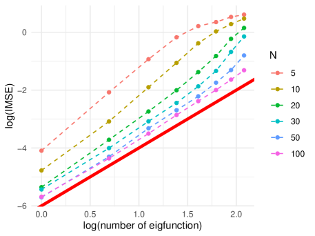
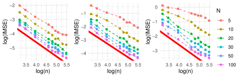
When the phase transition occurs, our theory indicates a proportional relationship such that for each fixed and for each fixed . Figure 1 illustrates this phenomenon by showing that as increases, the relationship between and tends to be linear with a slope of , indicating that the phase transition might occur around . Figure 1 additionally offers a practical way for identifying the phase transition point of . This is valuable in guiding both data collection and experimental design, contributing to more cost-effective data collecting strategies. Similarly, Figure 2 shows that as increases, the relationship between and also tends to follow a linear trend, but with a slope of .
7 Conclusion and discussion
In this paper, we focus on the convergence rate of eigenfunctions with diverging indices for discretely observed functional data. We propose new techniques to handle the perturbation series and establish sharp bounds for eigenvalues and eigenfunctions across different convergence types. Additionally, we extend the partition “dense” and “sparse” defined for mean and covariance functions to principal components analysis. Another notable contribution of this paper is the double truncation technique for handling uniform convergence. Existing results on uniform convergence for covariance estimation require a strong moment condition on and are only applicable to sparse functional data where . By employing the double truncation technique proposed in this paper, we establish an improved bound for the truncated bias, which ensures the uniform convergence of the covariance and eigenfunctions across all sampling schemes under mild conditions. These asymptotic properties play a direct role in various types of statistical inference involving functional data (Yao, Müller and Wang, 2005a; Li and Hsing, 2010).
Furthermore, the optimal rate achieved in this paper holds significant implications for downstream analysis. Since most functional regression models encounter inverse issues due to the infinite dimensionality of functional covariates, the convergence rates in this paper would help improve existing theoretical findings in downstream analyses from fully observed functional data to various sampling designs. Consider the functional linear model with . Without a sharp bound for eigenfunctions, achieving optimal convergence for standard and efficient plug-in estimators becomes challenging. Therefore, methods like approximated least squares and sample splitting, as discussed in (Zhou, Yao and Zhang, 2023), are necessary in the modeling phase. These complex methods require estimating principal components scores and do not efficiently utilize information gained from pooling. As a result, the phase transition for the functional linear model obtained by Zhou, Yao and Zhang (2023) is , which is significantly greater than . In contrast, by using the new results in this paper, one can directly apply the plug-in estimator from Hall and Horowitz (2007) and achieve a phase transition of for the functional linear model. Additionally, for complex regression models like the functional generalized linear model or functional Cox model, the methods developed in this paper could serve as a cornerstone for further exploration.
Proof of Theorem 1
Recall in the optimization problem (4) and has the analytical from
where
for and
Some calculations show that
and
where
In the following, we omit the arguments in the functions , , , and for and when there is no ambiguity. Simple calculations show that . We further denote
where is the density function of in the case of the random design, and in the case of the fixed regular design. The subsequent proof is structured into three steps to ensure clearer understanding.
Step 1: Discrepancy between and . The following lemma bound the discrepancy between and , and its proof can be found in Section S3 of the supplement.
Lemma 1.
Step 2: bound the projection . In this part, we will prove the following lemma, which provides expectation bounds for the projections of with respect to and .
Lemma 2.
Proof of Lemma 2.
We focus on the first statement of Lemma 2. The proof of the fix regular design is similar and we put it in supplement. By definition of , we need to bound the bias and variance terms of
| (15) |
For the random design case, by analogous calculation as proof of Theorem 3.2 in Zhang and Wang (2016), one has
where . Thus, for the bias part of equation (15), for all ,
| (16) | ||||
For the tail summation, similarly
| (17) | ||||
For the variance of equation (15), note that
| (18) | ||||
We start with the first term in the right hand side of equation (18). To simplify the notation, we shall introduce the following notation:
Then
with
By Cauchy–Schwarz and AM–GM inequality,
Similarly , thus, . Combine all above,
| (19) | ||||
The following lemma in bounding and , its proof can be found in the supplement.
By Lemma 3 and Cauchy-Schwarz inequality
| (20) | ||||
For , by Lemma 3 and Cauchy-Schwarz inequality,
| (21) |
For the summation , by Cauchy-Schwarz inequality
Thus,
| (22) | ||||
For the last term , note that
and
| (25) | ||||
Combine equation (20) to (25), for all
and
By similar analysis, the second term in the right hand side of equation (18) has the same convergence rate as the first term. Under and , the last two terms in the right hand side of equation (18) are dominated by the first two terms. Then the proof of the random design case is complete by
for all and
∎
Step 3: perturbation series. By the proof of Theorem 5.1.8 in Hsing and Eubank (2015), for and on the set , we have the following expansion,
| (26) | ||||
Such kind of expansion can also be found in Hall and Hosseini-Nasab (2006) and Li and Hsing (2010). Below, when we say that a bound is valid when holds, this should be interpreted as stating that the bound is valid for all realizations for which (Hall and Horowitz, 2007). Under assumptions , and , we have . Since implies , thus the results in form we want to prove relate only to probabilities of differences. It suffices to work with bounds that are established under the assumption such that holds. (Hall and Horowitz, 2007, Section 5.1).
We first show that is dominated by the norm of the first term in the right hand side of equation (26). By Bessel’s inequality, we see that
| (27) |
where the last equality comes from the fact on . Similarly,
| (28) | ||||
Combing (26) to (28) and the fact , is dominated by the first term in the right hand side of equation (26). Thus,
| (29) |
For the random design, under Assumption 6 and , by Bessel equality and (13), the first term in the right hand side of equation (29) is bounded by
The first statement of Theorem 1 is complete by
where the second inequality comes from Lemma 7 in Dou, Pollard and Zhou (2012) and Lemma 2. The proof for the fixed regular design is similar, and thus we omit the details for brevity.
References
- Anderson, Guionnet and Zeitouni (2010) {bbook}[author] \bauthor\bsnmAnderson, \bfnmGreg W\binitsG. W., \bauthor\bsnmGuionnet, \bfnmAlice\binitsA. and \bauthor\bsnmZeitouni, \bfnmOfer\binitsO. (\byear2010). \btitleAn Introduction to Random Matrices \bvolume118. \bpublisherCambridge university press. \endbibitem
- Bai and Silverstein (2010) {bbook}[author] \bauthor\bsnmBai, \bfnmZhidong\binitsZ. and \bauthor\bsnmSilverstein, \bfnmJack W\binitsJ. W. (\byear2010). \btitleSpectral Analysis of Large Dimensional Random Matrices \bvolume20. \bpublisherSpringer. \endbibitem
- Bai et al. (2009) {barticle}[author] \bauthor\bsnmBai, \bfnmZhidong\binitsZ., \bauthor\bsnmJiang, \bfnmDandan\binitsD., \bauthor\bsnmYao, \bfnmJian-Feng\binitsJ.-F. and \bauthor\bsnmZheng, \bfnmShurong\binitsS. (\byear2009). \btitleCorrections to LRT on large-dimensional covariance matrix by RMT. \bjournalAnn. Statist. \bvolume37 \bpages3822–3840. \endbibitem
- Bao et al. (2022) {barticle}[author] \bauthor\bsnmBao, \bfnmZhigang\binitsZ., \bauthor\bsnmDing, \bfnmXiucai\binitsX., \bauthor\bsnmWang, \bfnmJingming\binitsJ. and \bauthor\bsnmWang, \bfnmKe\binitsK. (\byear2022). \btitleStatistical inference for principal components of spiked covariance matrices. \bjournalAnn. Statist. \bvolume50 \bpages1144–1169. \endbibitem
- Bianchi et al. (2011) {barticle}[author] \bauthor\bsnmBianchi, \bfnmPascal\binitsP., \bauthor\bsnmDebbah, \bfnmMerouane\binitsM., \bauthor\bsnmMaïda, \bfnmMylène\binitsM. and \bauthor\bsnmNajim, \bfnmJamal\binitsJ. (\byear2011). \btitlePerformance of statistical tests for single-source detection using random matrix theory. \bjournalIEEE Trans. Inf. Theory. \bvolume57 \bpages2400–2419. \endbibitem
- Bickel and Rosenblatt (1973) {barticle}[author] \bauthor\bsnmBickel, \bfnmPeter J\binitsP. J. and \bauthor\bsnmRosenblatt, \bfnmMurray\binitsM. (\byear1973). \btitleOn some global measures of the deviations of density function estimates. \bjournalAnn. Statist. \bpages1071–1095. \endbibitem
- Bosq (2000) {bbook}[author] \bauthor\bsnmBosq, \bfnmDenis\binitsD. (\byear2000). \btitleLinear Processes in Function Spaces: Theory and Applications \bvolume149. \bpublisherSpringer Science & Business Media. \endbibitem
- Cai and Hall (2006) {barticle}[author] \bauthor\bsnmCai, \bfnmT Tony\binitsT. T. and \bauthor\bsnmHall, \bfnmPeter\binitsP. (\byear2006). \btitlePrediction in functional linear regression. \bjournalAnn. Statist. \bvolume34 \bpages2159–2179. \endbibitem
- Cai and Yuan (2010) {barticle}[author] \bauthor\bsnmCai, \bfnmTony\binitsT. and \bauthor\bsnmYuan, \bfnmMing\binitsM. (\byear2010). \btitleNonparametric covariance function estimation for functional and longitudinal data. \bjournalUniversity of Pennsylvania and Georgia inistitute of technology. \endbibitem
- Cai and Yuan (2011) {barticle}[author] \bauthor\bsnmCai, \bfnmT Tony\binitsT. T. and \bauthor\bsnmYuan, \bfnmMing\binitsM. (\byear2011). \btitleOptimal estimation of the mean function based on discretely sampled functional data: Phase transition. \bjournalAnn. Statist. \bvolume39 \bpages2330–2355. \endbibitem
- Chen and Qin (2010) {barticle}[author] \bauthor\bsnmChen, \bfnmSong Xi\binitsS. X. and \bauthor\bsnmQin, \bfnmYing-Li\binitsY.-L. (\byear2010). \btitleA two-sample test for high-dimensional data with applications to gene-set testing. \bjournalAnn. Statist. \bvolume38 \bpages808–835. \endbibitem
- Ding and Yang (2021) {barticle}[author] \bauthor\bsnmDing, \bfnmXiucai\binitsX. and \bauthor\bsnmYang, \bfnmFan\binitsF. (\byear2021). \btitleSpiked separable covariance matrices and principal components. \bjournalAnn. Statist. \bvolume49 \bpages1113–1138. \endbibitem
- Dou, Pollard and Zhou (2012) {barticle}[author] \bauthor\bsnmDou, \bfnmWinston Wei\binitsW. W., \bauthor\bsnmPollard, \bfnmDavid\binitsD. and \bauthor\bsnmZhou, \bfnmHarrison H\binitsH. H. (\byear2012). \btitleEstimation in functional regression for general exponential families. \bjournalAnn. Statist. \bvolume40 \bpages2421–2451. \endbibitem
- El Karoui (2007) {barticle}[author] \bauthor\bsnmEl Karoui, \bfnmNoureddine\binitsN. (\byear2007). \btitleTracy–Widom limit for the largest eigenvalue of a large class of complex sample covariance matrices. \bjournalAnn. Probab. \bvolume35 \bpages663–714. \endbibitem
- Ferraty and Vieu (2006) {bbook}[author] \bauthor\bsnmFerraty, \bfnmFrédéric\binitsF. and \bauthor\bsnmVieu, \bfnmPhilippe\binitsP. (\byear2006). \btitleNonparametric Functional Data Analysis: Theory and Practice. \bpublisherSpringer Science & Business Media. \endbibitem
- Hall and Horowitz (2007) {barticle}[author] \bauthor\bsnmHall, \bfnmPeter\binitsP. and \bauthor\bsnmHorowitz, \bfnmJoel L\binitsJ. L. (\byear2007). \btitleMethodology and convergence rates for functional linear regression. \bjournalAnn. Statist. \bvolume35 \bpages70–91. \endbibitem
- Hall and Hosseini-Nasab (2006) {barticle}[author] \bauthor\bsnmHall, \bfnmPeter\binitsP. and \bauthor\bsnmHosseini-Nasab, \bfnmMohammad\binitsM. (\byear2006). \btitleOn properties of functional principal components analysis. \bjournalJ. R. Stat. Soc. Ser. B Stat. Methodol. \bvolume68 \bpages109–126. \endbibitem
- Hall, Müller and Wang (2006) {barticle}[author] \bauthor\bsnmHall, \bfnmPeter\binitsP., \bauthor\bsnmMüller, \bfnmHans-Georg\binitsH.-G. and \bauthor\bsnmWang, \bfnmJane-Ling\binitsJ.-L. (\byear2006). \btitleProperties of principal component methods for functional and longitudinal data analysis. \bjournalAnn. Statist. \bpages1493–1517. \endbibitem
- Härdle (1989) {barticle}[author] \bauthor\bsnmHärdle, \bfnmWolfgang\binitsW. (\byear1989). \btitleAsymptotic maximal deviation of M-smoothers. \bjournalJ. Multivar. Anal. \bvolume29 \bpages163–179. \endbibitem
- Hardle, Janssen and Serfling (1988) {barticle}[author] \bauthor\bsnmHardle, \bfnmW\binitsW., \bauthor\bsnmJanssen, \bfnmPaul\binitsP. and \bauthor\bsnmSerfling, \bfnmRobert\binitsR. (\byear1988). \btitleStrong uniform consistency rates for estimators of conditional functionals. \bjournalAnn. Statist. \bpages1428–1449. \endbibitem
- Horváth and Kokoszka (2012) {bbook}[author] \bauthor\bsnmHorváth, \bfnmLajos\binitsL. and \bauthor\bsnmKokoszka, \bfnmPiotr\binitsP. (\byear2012). \btitleInference for Functional Data with Applications \bvolume200. \bpublisherSpringer Science & Business Media. \endbibitem
- Hsing and Eubank (2015) {bbook}[author] \bauthor\bsnmHsing, \bfnmTailen\binitsT. and \bauthor\bsnmEubank, \bfnmRandall\binitsR. (\byear2015). \btitleTheoretical Foundations of Functional Data Analysis, with an Introduction to Linear Operators \bvolume997. \bpublisherJohn Wiley & Sons. \endbibitem
- Indritz (1963) {bbook}[author] \bauthor\bsnmIndritz, \bfnmJack\binitsJ. (\byear1963). \btitleMethods in Analysis. \bpublisherMacmillan. \endbibitem
- Johnstone (2001) {barticle}[author] \bauthor\bsnmJohnstone, \bfnmIain M\binitsI. M. (\byear2001). \btitleOn the distribution of the largest eigenvalue in principal components analysis. \bjournalAnn. Statist. \bvolume29 \bpages295–327. \endbibitem
- Li and Hsing (2010) {barticle}[author] \bauthor\bsnmLi, \bfnmYehua\binitsY. and \bauthor\bsnmHsing, \bfnmTailen\binitsT. (\byear2010). \btitleUniform convergence rates for nonparametric regression and principal component analysis in functional/longitudinal data. \bjournalAnn. Statist. \bvolume38 \bpages3321–3351. \endbibitem
- Müller and Stadtmüller (2005) {barticle}[author] \bauthor\bsnmMüller, \bfnmHans-Georg\binitsH.-G. and \bauthor\bsnmStadtmüller, \bfnmUlrich\binitsU. (\byear2005). \btitleGeneralized functional linear models. \bjournalAnn. Statist. \bvolume33 \bpages774–805. \endbibitem
- Nadler, Penna and Garello (2011) {binproceedings}[author] \bauthor\bsnmNadler, \bfnmBoaz\binitsB., \bauthor\bsnmPenna, \bfnmFederico\binitsF. and \bauthor\bsnmGarello, \bfnmRoberto\binitsR. (\byear2011). \btitlePerformance of eigenvalue-based signal detectors with known and unknown noise level. In \bbooktitle2011 IEEE Int. Conf. Commun. \bpages1–5. \bpublisherIEEE. \endbibitem
- Onatski (2009) {barticle}[author] \bauthor\bsnmOnatski, \bfnmAlexei\binitsA. (\byear2009). \btitleTesting hypotheses about the number of factors in large factor models. \bjournalEconometrica \bvolume77 \bpages1447–1479. \endbibitem
- Pastur and Shcherbina (2011) {bbook}[author] \bauthor\bsnmPastur, \bfnmLeonid Andreevich\binitsL. A. and \bauthor\bsnmShcherbina, \bfnmMariya\binitsM. (\byear2011). \btitleEigenvalue Distribution of Large Random Matrices \bvolume171. \bpublisherAmerican Mathematical Soc. \endbibitem
- Paul (2007) {barticle}[author] \bauthor\bsnmPaul, \bfnmDebashis\binitsD. (\byear2007). \btitleAsymptotics of sample eigenstructure for a large dimensional spiked covariance model. \bjournalStat. Sinica. \bpages1617–1642. \endbibitem
- Paul and Aue (2014) {barticle}[author] \bauthor\bsnmPaul, \bfnmDebashis\binitsD. and \bauthor\bsnmAue, \bfnmAlexander\binitsA. (\byear2014). \btitleRandom matrix theory in statistics: A review. \bjournalJ. Stat. Plan. Inference. \bvolume150 \bpages1–29. \endbibitem
- Paul and Peng (2009) {barticle}[author] \bauthor\bsnmPaul, \bfnmDebashis\binitsD. and \bauthor\bsnmPeng, \bfnmJie\binitsJ. (\byear2009). \btitleConsistency of restricted maximum likelihood estimators of principal components. \bjournalAnn. Statist. \bvolume37 \bpages1229–1271. \endbibitem
- Qu, Wang and Wang (2016) {barticle}[author] \bauthor\bsnmQu, \bfnmSimeng\binitsS., \bauthor\bsnmWang, \bfnmJane-Ling\binitsJ.-L. and \bauthor\bsnmWang, \bfnmXiao\binitsX. (\byear2016). \btitleOptimal estimation for the functional cox model. \bjournalAnn. Statist. \bvolume44 \bpages1708–1738. \endbibitem
- Ramsay and Silverman (2006) {bbook}[author] \bauthor\bsnmRamsay, \bfnmJames\binitsJ. and \bauthor\bsnmSilverman, \bfnmBW\binitsB. (\byear2006). \btitleFunctional Data Analysis. \bpublisherSpringer Science & Business Media. \endbibitem
- Rice and Wu (2001) {barticle}[author] \bauthor\bsnmRice, \bfnmJohn A\binitsJ. A. and \bauthor\bsnmWu, \bfnmColin O\binitsC. O. (\byear2001). \btitleNonparametric mixed effects models for unequally sampled noisy curves. \bjournalBiometrics \bvolume57 \bpages253–259. \endbibitem
- Shao, Lin and Yao (2022) {barticle}[author] \bauthor\bsnmShao, \bfnmLingxuan\binitsL., \bauthor\bsnmLin, \bfnmZhenhua\binitsZ. and \bauthor\bsnmYao, \bfnmFang\binitsF. (\byear2022). \btitleIntrinsic Riemannian functional data analysis for sparse longitudinal observations. \bjournalAnn. Statist. \bvolume50 \bpages1696 – 1721. \bdoi10.1214/22-AOS2172 \endbibitem
- Wahl (2022) {binproceedings}[author] \bauthor\bsnmWahl, \bfnmMartin\binitsM. (\byear2022). \btitleLower bounds for invariant statistical models with applications to principal component analysis. In \bbooktitleAnn. Inst. Henri Poincaré Probab. Statist. \bvolume58 \bpages1565–1589. \bpublisherInstitut Henri Poincaré. \endbibitem
- Yao and Lee (2006) {barticle}[author] \bauthor\bsnmYao, \bfnmFang\binitsF. and \bauthor\bsnmLee, \bfnmThomas CM\binitsT. C. (\byear2006). \btitlePenalized spline models for functional principal component analysis. \bjournalJ. R. Stat. Soc. Ser. B Stat. Methodol. \bvolume68 \bpages3–25. \endbibitem
- Yao, Müller and Wang (2005a) {barticle}[author] \bauthor\bsnmYao, \bfnmFang\binitsF., \bauthor\bsnmMüller, \bfnmHans-Georg\binitsH.-G. and \bauthor\bsnmWang, \bfnmJane-Ling\binitsJ.-L. (\byear2005a). \btitleFunctional data analysis for sparse longitudinal data. \bjournalJ. Am. Stat. Assoc. \bvolume100 \bpages577–590. \endbibitem
- Yao, Müller and Wang (2005b) {barticle}[author] \bauthor\bsnmYao, \bfnmFang\binitsF., \bauthor\bsnmMüller, \bfnmHans-Georg\binitsH.-G. and \bauthor\bsnmWang, \bfnmJane-Ling\binitsJ.-L. (\byear2005b). \btitleFunctional linear regression analysis for longitudinal data. \bjournalAnn. Statist. \bpages2873–2903. \endbibitem
- Yuan and Cai (2010) {barticle}[author] \bauthor\bsnmYuan, \bfnmMing\binitsM. and \bauthor\bsnmCai, \bfnmT Tony\binitsT. T. (\byear2010). \btitleA reproducing kernel Hilbert space approach to functional linear regression. \bjournalAnn. Statist. \bvolume38 \bpages3412–3444. \endbibitem
- Zhang and Chen (2007) {barticle}[author] \bauthor\bsnmZhang, \bfnmJin-Ting\binitsJ.-T. and \bauthor\bsnmChen, \bfnmJianwei\binitsJ. (\byear2007). \btitleStatistical inferences for functional data. \bjournalAnn. Statist. \bvolume35 \bpages1052–1079. \endbibitem
- Zhang and Wang (2016) {barticle}[author] \bauthor\bsnmZhang, \bfnmXiaoke\binitsX. and \bauthor\bsnmWang, \bfnmJane-Ling\binitsJ.-L. (\byear2016). \btitleFrom sparse to dense functional data and beyond. \bjournalAnn. Statist. \bvolume44 \bpages2281–2321. \endbibitem
- Zheng (2012) {binproceedings}[author] \bauthor\bsnmZheng, \bfnmShurong\binitsS. (\byear2012). \btitleCentral limit theorems for linear spectral statistics of large dimensional -matrices. In \bbooktitleAnn. Inst. Henri Poincaré Probab. Statist \bvolume48 \bpages444–476. \endbibitem
- Zhou, Yao and Zhang (2023) {barticle}[author] \bauthor\bsnmZhou, \bfnmHang\binitsH., \bauthor\bsnmYao, \bfnmFang\binitsF. and \bauthor\bsnmZhang, \bfnmHuiming\binitsH. (\byear2023). \btitleFunctional linear regression for discretely observed data: from ideal to reality. \bjournalBiometrika \bvolume110 \bpages381–393. \endbibitem