Theoretical Studies
on Quantum Walks with a Time-varying Coin

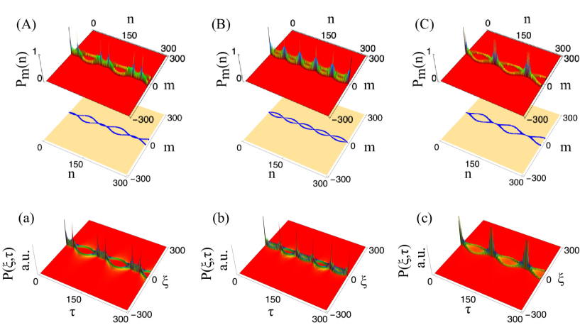
Numerical simulations are carried out by using $\theta(t)=\theta_{\_}0+\omega t$ as a specific time-dependent expression of the coin operator in Eq. (1) with various values for the initial phase $\theta_{\_}0$ and the frequency $\omega$. Figure 1 (A), (B) and (C) show the probability distributions of finding a walker on a line as a function of time under the identical frequency $\omega=\pi/60$ (upper panels) and their walker’s trajectories representing the place where the existence probability is high (lower panels). It is found that the time-varying coin leads to periodic walker’s trajectories classified into three types depending on the initial phase of the coin $\theta_{\_}0$: (1) Loop-line chain which is composed of loops and lines appearing alternately as shown in Fig. 1(A), (2) Crossing loop-loop chain where two major trajectories intersect as shown Fig. 1 (B), and (3) Touching loop-loop chain where two major trajectories come into contact as shown in Fig. 1 (C). In addition, walker’s trajectories are also modified by the frequency $\omega$. As the frequency $\omega$ increases, the size of the loops tends to become smaller in time and narrower in space (not displayed in Fig. 1).

In order to explore the physical origin of walker’s trajectories obtained by numerical simulations in the previous section, analytical probability distributions are obtained according to the method proposed by Knight, Roldán and Sipe[11]. Equations (6) and (7) are reduced to the following recurrence formula,

$\displaystyle A_{\_}{m,n+1}-A_{\_}{m,n-1}$

$\displaystyle=-\cos{\theta_{\_}n}(A_{\_}{m+1,n}-A_{\_}{m-1,n}),$

(10)

where $\theta_{\_}n=\theta_{\_}0+n\omega T$ and $A=R,L$. In the long-wavelength approximation, we obtain the wave equation for the continuous function $A(x,t)$

$\displaystyle T\frac{\partial}{\partial t}A(x,t)=-\cos{\theta(t)}\left(X\frac{\partial}{\partial x}+\frac{X^{3}}{3!}\frac{\partial^{3}}{\partial x^{3}}\right)A(x,t).$

(11)

where $X$ stands for the distance between steps. We further introduce other two fields $A^{+}(\xi,\tau)$ and $A^{-}(\xi,\tau)$ to express the waves spreading in both sides on a line, resulting in the wave equation

$\displaystyle\frac{\partial}{\partial\tau}A^{\pm}(\xi,\tau)=\mp\cos{\theta(\tau)}\left(\frac{\partial}{\partial\xi}+\frac{1}{3!}\frac{\partial^{3}}{\partial\xi^{3}}\right)A^{\pm}(\xi,\tau),$

(12)

where $\xi=x/X$ and $\tau=t/T$. This differential equation can be solved using Fourier techniques after separation of variables in a usual manner. The solution for Eq. (12) are given as follows

$\displaystyle A^{\pm}(\xi,\tau)$

$\displaystyle=\frac{1}{2}\sum_{\_}{m}(A_{\_}{m,0}\pm A_{\_}{m,1})Z^{\pm}(\xi-m,\tau),$

(13)

with

	$\displaystyle Z^{\pm}(\xi,\tau)$	$\displaystyle=\left|\frac{2}{s(\tau)}\right|^{\frac{1}{3}}e^{\chi}\operatorname{Ai}(\zeta),$		(14)
	$\displaystyle\zeta$	$\displaystyle=\left|\frac{2}{s(\tau)}\right|^{\frac{1}{3}}\left(\pm\xi-s(\tau)+\frac{2w^{4}}{s(\tau)}\right),$		(15)
	$\displaystyle\chi$	$\displaystyle=\frac{2w^{2}}{s(\tau)}\left(\pm\xi-s(\tau)+\frac{4w^{4}}{3s(\tau)}\right),$		(16)
	$\displaystyle s(\tau)$	$\displaystyle=\mp\int_{\_}{0}^{\tau}\cos{\theta(\tau^{\prime})}d\tau^{\prime},$		(17)

where $\operatorname{Ai}$ represents the Airy function. The probability distribution of finding a walker is then given by

	$\displaystyle P(\xi,\tau)$	$\displaystyle=P^{R}(\xi,\tau)+P^{L}(\xi,\tau),$		(18)
	$\displaystyle P^{A}(\xi,\tau)$	$\displaystyle=|A^{+}(\xi,\tau)+(-1)^{n}A^{-}(\xi,\tau)|^{2}.$		(19)

Figure 1 (a), (b) and (c) show probability distributions depicted by the analytic solution for the same value as coin parameters used in numerical simulations to (A), (B) and (C), respectively. Our analytical solution reproduces the numerical simulation well.

One definite example is as follows. Figure 2 shows the top view of the probability distributions obtained by the analytical solution (left) and the numerical simulation (right) at $\theta_{\_}0=0$ and $\omega=\pi/60$. According to the probability distribution given analytically in Eq.(18), the probability $P(\xi,\tau)$ is composed of $P^{R}(\xi,\tau)$ and $P^{L}(\xi,\tau)$. The highest probabilities in the analytical probability distribution are highlighted in blue ($P^{R}(\xi,\tau)$) and red ($P^{L}(\xi,\tau)$). The blue line and red line are exactly intersecting at $\tau=60$ with the same amplitude, resulting in a crossing loop-loop chain as seen in the numerical simulation. Actually, there exists a slight difference between analytical solutions and numerical simulations. Specifically, the amplitudes of the first and second loops differ only slightly in the graph on the left of Fig. 2. This is due to the approximation limit based on the wave nature of the quantum walk, i e., the nature of the Airy function. The maximum peak of the Airy function $\operatorname{Ai}(x)$ is not located at $x=0$, but at slightly negative position. As a result, the blue peak shifts more negatively than the dotted green line, and the red peak does the opposite. In other words, the maximum peak exists at the inside of the numerical loop at $\tau=30$, and outside at $\tau=90$ because the direction of the Airy function is reversed. This tiny difference causes only a few deviations. Thus, the analytical solution approximates the numerical simulation well. However, the linear spreading inherent in the quantum walk is not reproduced in the analytical solution and remains unsolved.

Despite the above better agreement, the probability distribution shown in Fig. 1 (b) may look different from that of numerical simulation shown in Fig. 1 (B). This difference is due to the Poggendorff illusion[9], which is a geometrical-optical illusion that involves the brain’s perception of the interaction between diagonal lines and horizontal and vertical edges. In fact, the probability of being inward in the first (left) loop and outward in the second (right) loop causes the Poggendorff illusion. In contrast, the numerical simulation does not show such a difference, resulting in no Poggendorff illusion. From the above, the analytic solution seemed to be different from the probability distribution of the numerical simulation, but in fact the analytic solution could approximate the numerical simulation correctly.

Now, let us discuss the walking mechanism based on the analytical solutions supported by numerical simulations obtained above. To find the walker’s trajectories which are a key clue for elucidating the walking mechanism, we examine the behavior of the probability amplitude $A^{\pm}(\xi,\tau)$, which is the main element that determines the probability distribution. The amplitude $A^{\pm}(\xi,\tau)$ is expressed as follows:

	$\displaystyle A^{\pm}(\xi,\tau)$	$\displaystyle=\int_{\_}{-\infty}^{\infty}e^{ik\xi}A^{\pm}(k,\tau)dk$
		$\displaystyle=B^{\pm}\left(\xi\mp\int_{\_}{0}^{\tau}\cos{\theta(\tau^{\prime})}d\tau^{\prime},\tau\right),$		(20)

where $B^{\pm}(\xi,\tau)$ represents a shifted probability amplitude described by

$\displaystyle B^{\pm}\left(\xi,\tau\right)=\int_{\_}{-\infty}^{\infty}e^{ik\xi}\left(e^{\pm\frac{1}{6}ik^{3}\int_{\_}{0}^{\tau}\cos{\theta(\tau^{\prime})}d\tau^{\prime}}A^{\pm}(k,0)\right)dk.$

(21)

Therefore, the walker’s trajectories is analytically obtained by the shift in Eq. (20) as follows:

	$\displaystyle x_{\_}c$	$\displaystyle=\mp\int_{\_}{0}^{\tau}\cos{\theta(\tau^{\prime})}d\tau^{\prime}$
		$\displaystyle=\mp\left(\frac{1}{\omega}\sin{(\theta_{\_}0+\omega\tau)}-\frac{1}{\omega}\sin{\theta_{\_}0}\right).$		(22)

Equation (22) means that walker’s trajectories are composed of two antisymmetric sinusoidal functions with same parameters such as amplitude $1/\omega$, initial phase $\theta_{\_}0$, frequency $\omega$, and bias $-\sin\theta_{\_}0/\omega$. The walker’s trajectories are formed by overlap of two sinusoidal waves, and are classified into three categories like loop-line chains, crossing loop-loop chains, and touching loop-loop chains as seen in numerical simulations. According to our simple overlap model, these three types of chains are interpreted as follows. Figure 3 (a) shows the first type of walker’s trajectories named ”loop-line chain”. In fact, two different size loops appear alternately though loop and line seemed to appear alternately. This type of chains is generated when the bias is finite except for $\theta_{\_}0=n\pi/2,(n=$integer). Figure 3 (b) shows the second type of walker’s trajectories, named ”crossing loop-loop chain”. This type of chains occurs when the bias is equal to 0, equivalently $\theta_{\_}0=n\pi$. Figure 3 (c) shows the third type of walker’s trajectories ”touching loop-loop chain”, which appears when the sinusoidal-wave amplitude equals its bias $(\theta_{\_}0=(2n+1)\pi/2)$. In this way, based on our analytical solution, it is found that walker’s trajectories are classified into three depending on the $\theta_{\_}0$ as obtained by numerical simulation.

The walker’s trajectories reflecting the walking mechanism reveal its physical origin. A trajectory is, in general, simply described by $\int v(t)dt$ wiht $v(t)$ being time-dependent velocity. According to wave theory, the velocity $v(t)$ works to connect the wave number $k$ (space) and frequency $\omega$ (time) through the well-known dispersion relation $\omega=vk$ in the linear wave. From our wave equation, Eq.(12), the term $\mp\cos{\theta(\tau)}$ corresponds to the wave velocity. In other words, the velocity that determines the trajectory is nothing but the transition amplitude of the coin itself. This shows that the time-varying coin parameter, i.e., the wave velocity, controls the walker’s trajectories. This is our central result of this paper.

References

- [1]
- [2] Y. Aharonov, L. Davidovich & N. Zagury (1993): Quantum random walks. Phys. Rev. A 48, pp. 1687–1690, 10.1103/PhysRevA.48.1687.
- [3] Francesca Albertini & Domenico D’Alessandro (2009): Analysis of quantum walks with time-varying coin on d-dimensional lattices. Journal of Mathematical Physics 50(12), p. 122106, 10.1063/1.3271109.
- [4] Mari-Carmen Bañuls, C. Navarrete, A. Pérez, Eugenio Roldán & J. Soriano (2006): Quantum Walk with a time-dependent coin. Physical Review A 73(6), 10.1103/PhysRevA.73.062304.
- [5] C. Cedzich & R. F. Werner (2016): Revivals in quantum walks with a quasiperiodically-time-dependent coin. Physical Review A 93(3), 10.1103/physreva.93.032329.
- [6] Tian Chen, Bo Wang & Xiangdong Zhang (2017): Controlling probability transfer in the discrete-time quantum walk by modulating the symmetries. New Journal of Physics 19(11), p. 113049, 10.1088/1367-2630/aa8fe4.
- [7] Andrew M. Childs (2009): Universal Computation by Quantum Walk. Phys. Rev. Lett. 102, p. 180501, 10.1103/PhysRevLett.102.180501.
- [8] Giuseppe Di Molfetta, Lauchlan Honter, Ben B. Luo, Tatsuaki Wada & Yutaka Shikano (2015): Massless Dirac equation from Fibonacci discrete-time quantum walk. Quantum Studies: Mathematics and Foundations 2(3), p. 243, 10.1007/s40509-015-0038-6.
- [9] Suzanne Greist-Bousquet & Harvey R Schiffman (1981): The Poggendorff Illusion: An Illusion of Linear Extent? Perception 10(2), pp. 155–164, 10.1068/p100155. PMID: 7279544.
- [10] Michal Karski, Leonid Förster, Jai-Min Choi, Andreas Steffen, Wolfgang Alt, Dieter Meschede & Artur Widera (2009): Quantum Walk in Position Space with Single Optically Trapped Atoms. Science 325(5937), pp. 174–177, 10.1126/science.1174436.
- [11] Peter L. Knight, Eugenio Roldán & J. E. Sipe (2004): Propagating quantum walks: The origin of interference structures. Journal of Modern Optics 51(12), p. 1761, 10.1080/09500340408232489.
- [12] Neil B. Lovett, Sally Cooper, Matthew Everitt, Matthew Trevers & Viv Kendon (2010): Universal quantum computation using the discrete-time quantum walk. Physical Review A 81(4), 10.1103/physreva.81.042330.
- [13] S Panahiyan & S Fritzsche (2018): Controlling quantum random walk with a step-dependent coin. New Journal of Physics 20(8), p. 083028, 10.1088/1367-2630/aad899.
- [14] Y. Shikano, T. Wada & J. Horikawa (2014): Discrete-time quantum walk with feed-forward quantum coin. Scientific Reports 4, 10.1038/srep04427.
- [15] Antoni Wójcik, Tomasz Łuczak, Paweł Kurzyński, Andrzej Grudka & Małgorzata Bednarska (2004): Quasiperiodic dynamics of a quantum walk on the line. Physical review letters 93(18), p. 180601, 10.1038/nature02008.
- [16] P. Xue, R. Zhang, H. Qin, X. Zhan, Z. H. Bian, J. Li & Barry C. Sanders (2015): Experimental Quantum-Walk Revival with a Time-Dependent Coin. Phys. Rev. Lett. 114, p. 140502, 10.1103/PhysRevLett.114.140502.
- [17] İskender Yalçınkaya & Zafer Gedik (2015): Qubit state transfer via discrete-time quantum walks. Journal of Physics A: Mathematical and Theoretical 48(22), p. 225302, 10.1088/1751-8113/48/22/225302.
- [18] Xiang Zhan, Hao Qin, Zhi-hao Bian, Jian Li & Peng Xue (2014): Perfect state transfer and efficient quantum routing: A discrete-time quantum-walk approach. Phys. Rev. A 90, p. 012331, 10.1103/PhysRevA.90.012331.