This paper was converted on www.awesomepapers.org from LaTeX by an anonymous user.
Want to know more? Visit the Converter page.

Theoretical Error Analysis of Entropy Approximation
for Gaussian Mixtures

Takashi Furuya Education and Research Center for Mathematical and Data Science, Shimane University, Japan Email: [email protected] Hiroyuki Kusumoto Equal contribution. Graduate School of Mathematics, Nagoya University, Japan Email: [email protected]
Koichi Taniguchi
Mathematical and Systems Engineering, Shizuoka University, Japan
Naoya Kanno Graduate School of Biomedical Engineering, Tohoku University, Japan Kazuma Suetake AISIN SOFTWARE, Japan
Abstract

Gaussian mixture distributions are commonly employed to represent general probability distributions. Despite the importance of using Gaussian mixtures for uncertainty estimation, the entropy of a Gaussian mixture cannot be calculated analytically. In this paper, we study the approximate entropy represented as the sum of the entropies of unimodal Gaussian distributions with mixing coefficients. This approximation is easy to calculate analytically regardless of dimension, but there is a lack of theoretical guarantees. We theoretically analyze the approximation error between the true and the approximate entropy to reveal when this approximation works effectively. This error is essentially controlled by how far apart each Gaussian component of the Gaussian mixture is. To measure such separation, we introduce the ratios of the distances between the means to the sum of the variances of each Gaussian component of the Gaussian mixture, and we reveal that the error converges to zero as the ratios tend to infinity. In addition, the probabilistic estimate indicates that this convergence situation is more likely to occur in higher-dimensional spaces. Therefore, our results provide a guarantee that this approximation works well for high-dimensional problems, such as neural networks that involve a large number of parameters.

Keywords : Gaussian mixture, Entropy approximation, Approximation error estimate, Upper and lower bounds

1 Introduction

Entropy is a fundamental measure of uncertainty in information theory with many applications in machine learning, data compression, and image processing. In machine learning, for instance, entropy is a key component in the evidence lower bound (ELBO) in the variational inference (Hinton and Van Camp, 1993; Barber and Bishop, 1998; Bishop, 2006) and the variational autoencoder (Kingma and Welling, 2013). It also plays a crucial role in the data acquisition for Bayesian optimization (Frazier, 2018) and active learning (Settles, 2009). In the real-world scenario, unimodal Gaussian distribution is widely used and offers computational advantages because its entropy can be calculated analytically, which offers computational advantages. However, unimodal Gaussian distributions are limited in the approximation ability, and in particular, they hardly approximate multimodal distributions, which are often assumed, for instance, as posterior distributions of Bayesian neural networks (BNNs) (MacKay, 1992; Neal, 2012) (see, e.g., Fort et al. (2019)). On the other hand, Gaussian mixture distribution (the superposition of Gaussian distributions) can capture the multimodality, and in general, approximate any continuous distribution in some topology (see, e.g., Bacharoglou (2010)). Unfortunately, the entropy of Gaussian mixture lacks a closed form, thereby necessitating the use of entropy approximation methods.

There are numerous approximation methods for estimating the entropy of Gaussian mixture (see Section 2). One common method for approximating the entropy of a Gaussian mixture is to compute the weighted sum of the entropies of the individual unimodal Gaussian components with mixing coefficients (see (3.2)), and this approximate entropy is easy to calculate analytically. However, despite its empirical success, this approximation lacks theoretical guarantees. The purpose of this paper is to reveal under what conditions this approximation performs well and to provide some theoretical insights on this approximation. Our contributions are as follows:

  • (Main result: New error bounds) We provide new upper and lower bounds of the approximation error. These bounds show that the error is essentially controlled by the ratios αk,k\alpha_{k,k^{\prime}} (which are given in Definition 4.1) of the distances between the means to the sum of the variances of each (Gaussian) component of the Gaussian mixture, and the error converges to zero as the ratios tend to infinity (Theorem 4.2). Consequently, we provide an “almost” necessary and sufficient condition for the approximate entropy to be valid (Remark 4.3).

  • (Probabilistic error bound) To confirm the effectiveness of the approximation for higher-dimension problems, we also provide the approximation error bound in the form of a probabilistic inequality (Corollary 4.7). In supplementary of Gal and Ghahramani (2016), it is mentioned (without mathematical proof) that this approximate entropy tends to be the true one in high-dimensional spaces when the means of the Gaussian mixture are randomly distributed. Our probabilistic inequality is a rigorous and generalized result of what they mention and shows the usefulness of this approximation in high-dimensional problems. Moreover, we numerically demonstrate this result in a simple case and show its superiority over several other methods (Section 5).

  • (Error bound for derivatives) For example in machine learning, not only the approximation of entropy but also its partial derivatives are required in backpropagation. Therefore, we also provide the upper bounds for the partial derivatives of the error with respect to parameters (Theorem 4.8), which ensure that the derivatives of the approximate entropy are also close enough to the true ones when the ratios are large enough.

  • (More detailed analysis in the special case) We conduct a more detailed analysis of the error bounds in a special case. More precisely, when all covariance matrices coincide, we provide an explicit formula on the entropy of Gaussian mixture with the integral dimension-reduced to its component number (Proposition 4.9). Then, by using this formula, we improve and simplify the upper and lower bounds of the error (Theorem 4.10) and the probabilistic inequality (Corollary 4.12). In this special case, we obtain a necessary and sufficient condition for this approximation to converge to the true entropy (Remark 4.11).

2 Related work

In numerical computation of the entropy of Gaussian mixtures, the approximation by Monte Carlo estimation is often used. However, it may require a large number of samples for high accuracy, leading to high computational costs. Furthermore, the Monte Carlo estimator gives a stochastic approximation, and hence, it does not guarantee deterministic bounds (confidence intervals may be used). There are numerous deterministic approximation methods (see, e.g., Hershey and Olsen (2007)). For example, approximation methods based on upper or lower bounds of the entropy are often used. That is, we try to obtain an approximation by estimating the upper or lower bounds of the entropy or we adopt the bounds as an approximate entropy (see, e.g., Bonilla et al. (2019); Hershey and Olsen (2007); Nielsen and Sun (2016); Zobay (2014)). A typical one is to use the lower bound of the entropy based on Jensen’s inequality (see Bonilla et al. (2019)). These approximations have the advantage of being analytically calculated in closed forms, whereas there is no theoretical guarantee that they work well in the context of machine learning such as variational inference. As another typical method, Huber et al. (2008) proposed the entropy approximation by a combination of the Taylor approximation with the splitting method of Gaussian mixture components. Recently, Dahlke and Pacheco (2023) provided new approximations using Taylor and Legendre series, and they theoretically and experimentally analyzed these approximations together with the approximation in Huber et al. (2008). Notably, Dahlke and Pacheco (2023) theoretically showed sufficient conditions for the approximations to be convergent. However, their performance remains unexplored in higher-dimensional cases. As an approximation that is easy to calculate regardless of dimensions, the sum of the entropies of unimodal Gaussian distributions is often used. For example, the approximation entropy represented as the “sum with mixing coefficients” of the entropies of unimodal Gaussian distributions (see Remark 4.5), which is equal to the true one when all Gaussian components coincide, is investigated in Melbourne et al. (2022). On the other hand, Gal and Ghahramani (2016) used the approximation represented as the sum of the entropies of “unimodal Gaussian distributions with mixture coefficients” in the context of variational inference from an intuition that this approximation tends to the true one in high-dimensional spaces when the means of the mixture are randomly distributed. In our work, we focus on the theoretical error estimation for this approximation and reveal that this approximation converges to the true one when all Gaussian components are far apart or in high-dimensional cases.

3 Entropy approximation for Gaussian mixtures

The entropy of probability distribution q(w)q(w) is defined by

H[q]mq(w)log(q(w))𝑑w.\displaystyle H[q]\coloneqq-\int_{\mathbb{R}^{m}}q(w)\log(q(w))\,dw. (3.1)

Here, we choose a probability distribution q(w)q(w) as the Gaussian mixture distribution, that is,

q(w)=k=1Kπk𝒩(w|μk,Σk),wm,q(w)=\sum_{k=1}^{K}\pi_{k}\mathcal{N}(w\,|\,\mu_{k},\Sigma_{k}),\quad w\in\mathbb{R}^{m},

where KK\in\mathbb{N} is the number of mixture components, and πk(0,1]\pi_{k}\in(0,1] are mixing coefficients constrained by k=1Kπk=1\sum_{k=1}^{K}\pi_{k}=1. Here, 𝒩(μk,Σk)=𝒩(w|μk,Σk)\mathcal{N}(\mu_{k},\Sigma_{k})=\mathcal{N}(w\,|\,\mu_{k},\Sigma_{k}) is the Gaussian distribution with a mean μkm\mu_{k}\in\mathbb{R}^{m} and (positive definite) covariance matrix Σkm×m\Sigma_{k}\in\mathbb{R}^{m\times m}, that is,

𝒩(w|μk,Σk)=1(2π)m|Σk|exp(12wμkΣk2),\mathcal{N}(w\,|\,\mu_{k},\Sigma_{k})=\frac{1}{\sqrt{(2\pi)^{m}|\Sigma_{k}|}}\exp\left(-\frac{1}{2}\left\|w-\mu_{k}\right\|_{\Sigma_{k}}^{2}\right),

where |Σk||\Sigma_{k}| is the determinant of matrix Σk\Sigma_{k}, and xΣ2x(Σ1x)\|x\|_{\Sigma}^{2}\coloneqq x\cdot(\Sigma^{-1}x) for a vector xmx\in\mathbb{R}^{m} and a positive definite matrix Σm×m\Sigma\in\mathbb{R}^{m\times m}. However, the entropy term H[q]H[q] cannot be computed analytically when the distribution q(w)q(w) is a Gaussian mixture.

We define the approximate entropy H~[q]\widetilde{H}[q] by the sum of the entropies of “unimodal Gaussian distributions with mixture coefficients”:

H~[q]k=1Kmπk𝒩(w|μk,Σk)log(πk𝒩(w|μk,Σk))𝑑w=m2+m2log2π+12k=1Kπklog|Σk|k=1Kπklogπk,\begin{split}\widetilde{H}[q]\coloneqq&\,-\sum_{k=1}^{K}\int_{\mathbb{R}^{m}}\pi_{k}\mathcal{N}(w\,|\,\mu_{k},\Sigma_{k})\log\left(\pi_{k}\mathcal{N}(w\,|\,\mu_{k},\Sigma_{k})\right)dw\\ =&\,\frac{m}{2}+\frac{m}{2}\log 2\pi+\frac{1}{2}\sum_{k=1}^{K}\pi_{k}\log|\Sigma_{k}|-\sum_{k=1}^{K}\pi_{k}\log\pi_{k},\end{split} (3.2)

which can be computed analytically. It is obvious that H[q]=H~[q]H[q]=\widetilde{H}[q] holds for unimodal Gaussian (i.e., the case K=1K=1). Moreover, it is shown that

0H~[q]H[q]2k=1Kπklogπk(2logK)0\leq\widetilde{H}[q]-H[q]\leq-2\sum_{k=1}^{K}\pi_{k}\log\pi_{k}\ (\leq 2\log K)

(see (LABEL:computation1) in Appendix and Remark 4.5). These bounds show that the error does not blow up with respect to the mean μk\mu_{k}, the covariance Σk\Sigma_{k}, and the dimension mm if the number of mixture components KK is fixed. In addition, these bounds imply that |H~[q]H[q]|0|\widetilde{H}[q]-H[q]|\to 0 as the Gaussian mixture qq converges to a unimodal Gaussian (i.e., πk1\pi_{k}\to 1 for some kk and πk0\pi_{k^{\prime}}\to 0 for all kkk^{\prime}\not=k). It is natural to ask under what other conditions this approximation H[q]H~[q]H[q]\approx\widetilde{H}[q] can be justified. In Section 4, we will provide an “almost” necessary and sufficient condition for this approximation to be valid.

4 Theoretical error analysis of the entropy approximation

In this section, we analyze the approximation error |H[q]H~[q]||H[q]-\widetilde{H}[q]| to theoretically justify the entropy approximation H~[q]H[q]\widetilde{H}[q]\approx H[q].

We introduce the following notation to state our results.

Definition 4.1.

For two Gaussian distributions 𝒩(μk,Σk)\mathcal{N}(\mu_{k},\Sigma_{k}) and 𝒩(μk,Σk)\mathcal{N}(\mu_{k^{\prime}},\Sigma_{k^{\prime}}), we define α{k,k}\alpha_{\{k,k^{\prime}\}} by

α{k,k}max{α>0:{xm:xμkΣk<α}{xm:xμkΣk<α}=},\alpha_{\{k,k^{\prime}\}}\coloneqq\max\Big{\{}\alpha>0:\{x\in\mathbb{R}^{m}:\|x-\mu_{k}\|_{\Sigma_{k}}<\alpha\}\cap\{x\in\mathbb{R}^{m}:\|x-\mu_{k^{\prime}}\|_{\Sigma_{k^{\prime}}}<\alpha\}=\varnothing\Big{\}}, (4.1)

and αk,k\alpha_{k,k^{\prime}} by

αk,kμkμkΣk1+Σk12Σk12op,\alpha_{k,k^{\prime}}\coloneqq\frac{\|\mu_{k}-\mu_{k^{\prime}}\|_{\Sigma_{k}}}{1+\|\Sigma_{k}^{-\frac{1}{2}}\Sigma_{k^{\prime}}^{\frac{1}{2}}\|_{\rm op}}, (4.2)

where k,k[K]{1,,K}k,k^{\prime}\in[K]\coloneqq\{1,\ldots,K\} and op\|\cdot\|_{\rm op} is the operator norm (i.e., the largest singular value).

Interpretation of α\alpha: We can interpret that α{k,k}\alpha_{\{k,k^{\prime}\}} and αk,k\alpha_{k,k^{\prime}} measure distances of two Gaussian distributions in some sense respectively. Here notice that α{k,k}\alpha_{\{k,k^{\prime}\}} is symmetric (i.e., α{k,k}\alpha_{\{k,k^{\prime}\}} is always equal to α{k,k}\alpha_{\{k^{\prime},k\}}), but αk,k\alpha_{k,k^{\prime}} is not necessarily symmetric (i.e., αk,k\alpha_{k,k^{\prime}} is not always equal to αk,k\alpha_{k^{\prime},k}).

Figure 1 shows the geometric interpretation of αk,k\alpha_{k,k^{\prime}} in the isotropic case, that is, Σk=σk2I\Sigma_{k}=\sigma^{2}_{k}I and Σk=σk2I\Sigma_{k^{\prime}}=\sigma^{2}_{k^{\prime}}I. In this case, αk,k\alpha_{k,k^{\prime}} has a symmetric form with respect to k,kk,k^{\prime} as

α{k,k}=αk,k=αk,k=|μkμk|σk+σk.\alpha_{\{k,k^{\prime}\}}=\alpha_{k,k^{\prime}}=\alpha_{k^{\prime},k}=\frac{|\mu_{k}-\mu_{k^{\prime}}|}{\sigma_{k}+\sigma_{k^{\prime}}}.

Here, the volume of 𝒩(μk,σk2I)\mathcal{N}(\mu_{k},\sigma_{k}^{2}I) on B(μk,ασk)B(\mu_{k},\alpha\sigma_{k}) is equal to that of 𝒩(μk,σk2I)\mathcal{N}(\mu_{k^{\prime}},\sigma_{k^{\prime}}^{2}I) on B(μk,ασk)B(\mu_{k^{\prime}},\alpha\sigma_{k^{\prime}}), where B(μ,σ){xm:|xμ|<σ}B(\mu,\sigma)\coloneqq\{x\in\mathbb{R}^{m}:|x-\mu|<\sigma\} for μm\mu\in\mathbb{R}^{m} and σ>0\sigma>0. If all distances |μkμk||\mu_{k}-\mu_{k^{\prime}}| between the means go to infinity, or all variances σk\sigma_{k} go to zero, etc., then αk,k\alpha_{k,k^{\prime}} go to infinity for all pairs of k,kk,k^{\prime}. Furthermore, if all means μk\mu_{k} are normally distributed (variances σk\sigma_{k} are fixed), then an expected value of αk,k2\alpha_{k,k^{\prime}}^{2} is in proportion to the dimension mm. That intuitively means that the expected value of αk,k\alpha_{k,k^{\prime}} becomes large as the dimension mm of the parameter increases.

Refer to caption
Figure 1: Illustration of α=α{k,k}\alpha=\alpha_{\{k,k^{\prime}\}} (m=2m=2, isotropic)
Refer to caption
Refer to caption
Figure 2: Illustration of α=αk,k\alpha=\alpha_{k,k^{\prime}} (m=2m=2, anisotropic, σ=Σk12Σk12op)\sigma=\|\Sigma_{k}^{-\frac{1}{2}}\Sigma_{k^{\prime}}^{\frac{1}{2}}\|_{\rm op})

These intuitions also hold in anisotropic case. From definition (4.2), we have

αk,k+αk,kΣk12Σk12op=|Σk12μkΣk12μk|.\alpha_{k,k^{\prime}}+\alpha_{k,k^{\prime}}\|\Sigma_{k}^{-\frac{1}{2}}\Sigma_{k^{\prime}}^{\frac{1}{2}}\|_{\rm op}=|\Sigma_{k}^{-\frac{1}{2}}\mu_{k}-\Sigma_{k}^{-\frac{1}{2}}\mu_{k^{\prime}}|.

This shows that the circumsphere of {xm:xΣk12μkΣk1Σk<αk,k}\{x\in\mathbb{R}^{m}:\|x-\Sigma_{k}^{-\frac{1}{2}}\mu_{k^{\prime}}\|_{\Sigma_{k}^{-1}\Sigma_{k}^{\prime}}<\alpha_{k,k^{\prime}}\} circumscribes B(Σk12μk,α)B(\Sigma_{k}^{-\frac{1}{2}}\mu_{k},\alpha) (see Figure 2 right). Moreover, by coordinate transformation xΣk12xx\to\Sigma_{k}^{\frac{1}{2}}x, we can interpret that αk,k\alpha_{k,k^{\prime}} is a distance of 𝒩(μk,Σk)\mathcal{N}(\mu_{k},\Sigma_{k}) and 𝒩(μk,Σk)\mathcal{N}(\mu_{k^{\prime}},\Sigma_{k^{\prime}}) from the perspective of Σk\Sigma_{k} (see Figure 2 left), and αk,k\alpha_{k,k^{\prime}} gives a concrete form of α\alpha satisfying {xμkΣk<α}{xμkΣk<α}={\{\|x-\mu_{k}\|_{\Sigma_{k}}<\alpha\}\cap\{\|x-\mu_{k^{\prime}}\|_{\Sigma_{k^{\prime}}}<\alpha\}=\varnothing}, that is, αk,kα{k,k}\alpha_{k,k^{\prime}}\leq\alpha_{\{k,k^{\prime}\}} (Lemma A.4).

4.1 General covariance case

We study the error |H[q]H~[q]||H[q]-\widetilde{H}[q]| for general covariance matrices Σk\Sigma_{k}. First, we give the following upper and lower bounds for the error.

Theorem 4.2.

Let s[0,1)s\in[0,1). Then

k=1Kkkπkπk1πkck,klog(1+1πkπk|Σk|12maxl|Σl|12exp((1+Σk12Σk12op)22αk,k2))|H[q]H~[q]|2(1s)m4k=1Kkkπkπkexp(sαk,k24),\begin{split}&\sum_{k=1}^{K}\sum_{k^{\prime}\neq k}\frac{\pi_{k}\pi_{k^{\prime}}}{1-\pi_{k}}c_{k,k^{\prime}}\log\Biggl{(}1+\frac{1-\pi_{k}}{\pi_{k}}\frac{|\Sigma_{k}|^{\frac{1}{2}}}{\displaystyle\max_{l}|\Sigma_{l}|^{\frac{1}{2}}}\exp\Biggl{(}-\frac{\Bigl{(}1+\|\Sigma_{k^{\prime}}^{-\frac{1}{2}}\Sigma_{k}^{\frac{1}{2}}\|_{\rm op}\Bigr{)}^{2}}{2}\alpha_{k^{\prime},k}^{2}\Biggr{)}\Biggr{)}\\ &\leq\left|H[q]-\widetilde{H}[q]\right|\leq\frac{2}{(1-s)^{\frac{m}{4}}}\sum_{k=1}^{K}\sum_{k^{\prime}\neq k}\sqrt{\pi_{k}\pi_{k^{\prime}}}\exp\left(-\frac{s\alpha_{k,k^{\prime}}^{2}}{4}\right),\end{split} (4.3)

where the coefficient ck,kc_{k,k^{\prime}} is defined by

ck,k1(2π)mk,kmexp(|y|22)𝑑y0,c_{k,k^{\prime}}\coloneqq\frac{1}{\sqrt{(2\pi)^{m}}}\int_{\mathbb{R}^{m}_{k,k^{\prime}}}\exp\left(-\frac{|y|^{2}}{2}\right)dy\geq 0,

and the set k,km\mathbb{R}^{m}_{k,k^{\prime}} is defined by

k,km{ym:yy(Σk12Σk1Σk12y)y,y(Σk12Σk1(μkμk))0}.\mathbb{R}^{m}_{k,k^{\prime}}\coloneqq\left\{y\in\mathbb{R}^{m}:\begin{array}[]{cc}y\cdot y\geq(\Sigma_{k}^{\frac{1}{2}}\Sigma_{k^{\prime}}^{-1}\Sigma_{k}^{\frac{1}{2}}y)\cdot y,\\ y\cdot(\Sigma_{k}^{\frac{1}{2}}\Sigma_{k^{\prime}}^{-1}(\mu_{k^{\prime}}-\mu_{k}))\geq 0\end{array}\right\}.

Moreover, the same upper bound holds for α{k,k}\alpha_{\{k,k^{\prime}\}} instead of αk,k\alpha_{k,k^{\prime}}:

|H[q]H~[q]|2(1s)m4k=1Kkkπkπkexp(sα{k,k}24).\left|H[q]-\widetilde{H}[q]\right|\leq\frac{2}{(1-s)^{\frac{m}{4}}}\sum_{k=1}^{K}\sum_{k^{\prime}\neq k}\sqrt{\pi_{k}\pi_{k^{\prime}}}\exp\left(-\frac{s\alpha_{\{k,k^{\prime}\}}^{2}}{4}\right). (4.4)

The proof is given by calculations with the triangle inequality, the Cauchy-Schwarz inequality, and a change of variables. For upper bound, we use the inequality log(1+x)x\log(1+x)\leq\sqrt{x} (x0)(x\geq 0), and we split the integral region to |y|<αk,k|y|<\alpha_{k,k^{\prime}} and |y|>αk,k|y|>\alpha_{k,k^{\prime}} in order to utilize the characteristic of αk,k\alpha_{k,k^{\prime}}. While, for the lower bound, we use the concavity of function xlog(1+x)x\mapsto\log(1+x) (x>0)(x>0) and the definition of k,km\mathbb{R}^{m}_{k,k^{\prime}}. See Appendix A.1 for the proof of Theorem 4.2.

Remark 4.3.

Theorem 4.2 implies the following facts:

  • (i)

    According to the upper bound in (4.3), the approximation H[q]H~[q]H[q]\approx\widetilde{H}[q] is valid when

    • (a)

      πkπk0\pi_{k}\pi_{k^{\prime}}\to 0 or αk,k+\alpha_{k,k^{\prime}}\to+\infty for all pairs k,k[K]k,k^{\prime}\in[K] with kkk\neq k^{\prime}

    for s(0,1)s\in(0,1). In particular, the error exponentially decays to zero when all αk,k\alpha_{k,k^{\prime}} go to zero.

  • (ii)

    According to the upper bound (4.4), the approximation H[q]H~[q]H[q]\approx\widetilde{H}[q] is also valid when

    • (b)

      πkπk0\pi_{k}\pi_{k^{\prime}}\to 0 or α{k,k}+\alpha_{\{k,k^{\prime}\}}\to+\infty for all pairs k,k[K]k,k^{\prime}\in[K] with kkk\neq k^{\prime}

    for s(0,1)s\in(0,1). Moreover, the upper bound in (4.4) is better than that in (4.3) since αk,kα{k,k}\alpha_{k,k^{\prime}}\leq\alpha_{\{k,k^{\prime}\}} always holds (see Lemma A.4).

  • (iii)

    According to the lower bound in (4.3), if ck,k>0c_{k,k^{\prime}}>0 and Σk12Σk12opC\|\Sigma_{k^{\prime}}^{-\frac{1}{2}}\Sigma_{k}^{\frac{1}{2}}\|_{\rm op}\leq C hold for all pairs k,kk,k^{\prime} and some constant C>0C>0 independent of k,kk,k^{\prime}, then (a) is necessary for this approximation to be valid (where we note that |Σk|12/|Σk|12=|Σk12Σk12|Cm|\Sigma_{k}|^{\frac{1}{2}}/|\Sigma_{k^{\prime}}|^{\frac{1}{2}}=|\Sigma_{k^{\prime}}^{-\frac{1}{2}}\Sigma_{k}^{\frac{1}{2}}|\leq C^{m} when Σk12Σk12opC\|\Sigma_{k^{\prime}}^{-\frac{1}{2}}\Sigma_{k}^{\frac{1}{2}}\|_{\rm op}\leq C, and that mink|Σk|12/maxk|Σk|12Cm\min_{k}|\Sigma_{k}|^{\frac{1}{2}}/\max_{k}|\Sigma_{k}|^{\frac{1}{2}}\geq C^{-m} holds). It is unclear whether all ck,kc_{k,k^{\prime}} are positive, but we can show that either ck,kc_{k,k^{\prime}} or ck,kc_{k^{\prime},k} is always positive for any pair k,kk,k^{\prime} (see Remark A.6).

  • (iv)

    From the above facts and the symmetry of α{k,k}\alpha_{\{k,k^{\prime}\}}, we conclude that (b) is a necessary and sufficient condition for the approximation H[q]H~[q]H[q]\approx\widetilde{H}[q] to be valid if Σk12Σk12opC\|\Sigma_{k^{\prime}}^{-\frac{1}{2}}\Sigma_{k}^{\frac{1}{2}}\|_{\rm op}\leq C hold for all pairs k,kk,k^{\prime} and some constant C>0C>0 independent of k,kk,k^{\prime}.

Remark 4.4.

In Theorem 4.2, the parameter ss plays a role of adjusting the convergence speed as follows:

  1. (i)

    In the case of s=0s=0, the upper bound does not imply the convergence, and the following bound is obtained:

    |H[q]H~[q]|2k=1Kkkπkπkk=1Kkk(πk+πk)=k=1K{(K1)πk+(1πk)}=2(K1).\left|H[q]-\widetilde{H}[q]\right|\leq 2\sum_{k=1}^{K}\sum_{k^{\prime}\neq k}\sqrt{\pi_{k}\pi_{k^{\prime}}}\leq\sum_{k=1}^{K}\sum_{k^{\prime}\neq k}(\pi_{k}+\pi_{k}^{\prime})=\sum_{k=1}^{K}\{(K-1)\pi_{k}+(1-\pi_{k})\}=2(K-1).
  2. (ii)

    Consider the upper bound (focusing on the term of k,kk,k^{\prime} pair in summation) of (4.3) as a function with respect to ss, it is minimal on s=1m/αk,k2s=1-m/\alpha_{k,k^{\prime}}^{2} if αk,km\alpha_{k,k^{\prime}}\geq\sqrt{m}, and monotonically increase in s[0,1)s\in[0,1) if αk,k<m\alpha_{k,k^{\prime}}<\sqrt{m}. Replacing ss on each k,kk,k^{\prime} summation in the proof of Theorem 4.2 with minimal points sk,k=1m/αk,k2s_{k,k^{\prime}}=1-m/\alpha_{k,k^{\prime}}^{2}, we obtain more precise upper bound

    |H[q]H~[q]|2k=1Kkkπkπk(αk,k2m)m4exp(mαk,k24),\left|H[q]-\widetilde{H}[q]\right|\leq 2\sum_{k=1}^{K}\sum_{k^{\prime}\neq k}\sqrt{\pi_{k}\pi_{k^{\prime}}}\left(\frac{\alpha_{k,k^{\prime}}^{2}}{m}\right)^{\frac{m}{4}}\exp\left(\frac{m-\alpha_{k,k^{\prime}}^{2}}{4}\right),

    which converges to zero when dimension mm goes to infinity, if αk,k>m\alpha_{k,k^{\prime}}>\sqrt{m} for all pairs k,kk,k^{\prime}.

Remark 4.5.

Melbourne et al. (2022) has explored the entropy approximation of mixtures represented as the “sum with mixing coefficients” of the entropies of unimodal Gaussian distributions (without mixing coefficients in the logarithmic term):

H~Melbourne[q]k=1Kπkm𝒩(w|μk,Σk)log(𝒩(w|μk,Σk))𝑑w=H~[q]+k=1Kπklogπk.\widetilde{H}_{\rm Melbourne}[q]\coloneqq-\sum_{k=1}^{K}\pi_{k}\int_{\mathbb{R}^{m}}\mathcal{N}(w\,|\,\mu_{k},\Sigma_{k})\log\left(\mathcal{N}(w\,|\,\mu_{k},\Sigma_{k})\right)dw=\widetilde{H}[q]+\sum_{k=1}^{K}\pi_{k}\log\pi_{k}. (4.5)

This approximate entropy is equal to the true entropy H[q]H[q] when all Gaussian components coincide (i.e., μk=μk\mu_{k}=\mu_{k^{\prime}} and Σk=Σk\Sigma_{k}=\Sigma_{k^{\prime}} for all k,k[K])(k,k^{\prime}\in[K])(see (Melbourne et al., 2022, Theorem I.1)), but not when all Gaussian components are far apart (i.e., αk,k\alpha_{k,k^{\prime}}\to\infty for all k,k[K]k,k^{\prime}\in[K]). In contrast, while the approximation H~[q]\widetilde{H}[q] differs from H[q]H[q] when all Gaussian components coincide, it converges to H[q]H[q] when all Gaussian components are far apart (see Theorem 4.2). This is because H~Melbourne[q]\widetilde{H}_{\rm Melbourne}[q] differs by k=1Kπklogπk-\sum_{k=1}^{K}\pi_{k}\log\pi_{k} from H~[q]\widetilde{H}[q] (refer to (3.2)). Moreover, using also Wang and Madiman (2014, Lemma XI.2), the other upper bound

|H[q]H~[q]||H[q]HMelbourne[q]|+|HMelbourne[q]H~[q]|2k=1Kπklogπk2logK\left|H[q]-\widetilde{H}[q]\right|\leq\Bigl{|}H[q]-H_{\rm Melbourne}[q]\Bigr{|}+\left|H_{\rm Melbourne}[q]-\widetilde{H}[q]\right|\leq-2\sum_{k=1}^{K}\pi_{k}\log\pi_{k}\leq 2\log K (4.6)

is obtained, where the last inequality is justified by constraint k=1Kπk=1\sum_{k=1}^{K}\pi_{k}=1.

Remark 4.6.

In Lemma A.1, we obtain another upper bound K/2K/2, which is slightly better than 2logK2\log K in (4.6) when 2K82\leq K\leq 8.

Next, we provide the probabilistic inequality for the error as a corollary of Theorem 4.2.

Corollary 4.7.

Let c>0c>0. Take {μk}k\{\mu_{k}\}_{k} and {Σk}k\{\Sigma_{k}\}_{k} such that

Σk12(μkμk)1+Σk12Σk12op𝒩(0,c2I)\frac{\Sigma_{k}^{-\frac{1}{2}}(\mu_{k}-\mu_{k^{\prime}})}{1+\|\Sigma_{k}^{-\frac{1}{2}}\Sigma_{k^{\prime}}^{\frac{1}{2}}\|_{\rm op}}\sim\mathcal{N}(0,c^{2}I) (4.7)

for all pairs k,k[K]k,k^{\prime}\in[K] (kkk\neq k^{\prime}), that is, the left-hand side follows a Gaussian distribution with zero mean and an isotropic covariance matrix c2Ic^{2}I. Then, for ε>0\varepsilon>0 and s(0,1)s\in(0,1),

P(|H[q]H~[q]|ε)2(K1)ε(1s(1+sc22))m2.\begin{split}&P\left(\left|H[q]-\widetilde{H}[q]\right|\geq\varepsilon\right)\leq\frac{2(K-1)}{\varepsilon}\left(\sqrt{1-s}\left(1+\frac{sc^{2}}{2}\right)\right)^{-\frac{m}{2}}.\end{split} (4.8)

The proof is a combination of Markov’s inequality and the upper bound in Theorem 4.2. We also use the moment generating function of αk,k2/c2\alpha_{k,k^{\prime}}^{2}/c^{2} which follows the χ2\chi^{2}-distribution by the assumption (4.7). See Appendix A.2 for the details.

When (4.7) holds, an expected value of αk,k2\alpha^{2}_{k,k^{\prime}} is c2mc^{2}m. Hence, if αk,k2\alpha^{2}_{k,k^{\prime}} is regarded as c2mc^{2}m, then for c>1c>1 there exists s(0,1)s\in(0,1) such that the upper bound in (4.3) expectedly converges to zero as the dimension mm goes to infinity. Furthermore, Corollary 4.7 justifies Gal and Ghahramani (2016, Proposition 1 in Appendix A), which formally mentions that H~[q]\widetilde{H}[q] tends to H[q]H[q] when means μk\mu_{k} are normally distributed, all elements of covariance matrices Σk\Sigma_{k} do not depend on mm, and mm is large enough. In fact, the right-hand side of (4.8) converges to zero as mm\to\infty for some s(0,1)s\in(0,1) if c>1c>1.

We also study the derivatives of the error |H[q]H~[q]||H[q]-\widetilde{H}[q]| with respect to learning parameters θ=(πk,μk,Σk)k=1K\theta=(\pi_{k},\mu_{k},\Sigma_{k})_{k=1}^{K}. For simplicity, we write

ΓkΣk12.\Gamma_{k}\coloneqq\Sigma^{\frac{1}{2}}_{k}.

We give the following upper bounds for the derivatives of the error.

Theorem 4.8.

Let k[K]k\in[K], p,q[m]p,q\in[m], and s(0,1)s\in(0,1). Then

(i)\displaystyle\mathrm{(i)} |μk,p(H[q]H~[q])|2(1s)m+24kkπkπk(Γk11+Γk11)exp(sαk,k24),\displaystyle\quad\left|\frac{\partial}{\partial\mu_{k,p}}\left(H[q]-\widetilde{H}[q]\right)\right|\leq\frac{2}{(1-s)^{\frac{m+2}{4}}}\sum_{k^{\prime}\neq k}\sqrt{\pi_{k}\pi_{k^{\prime}}}\left(\left\|\Gamma_{k^{\prime}}^{-1}\right\|_{1}+\left\|\Gamma_{k}^{-1}\right\|_{1}\right)\exp\left(-\frac{s\alpha_{k,k^{\prime}}^{2}}{4}\right),
(ii)\displaystyle\mathrm{(ii)} |γk,pq(H[q]H~[q])|\displaystyle\quad\left|\frac{\partial}{\partial\gamma_{k,pq}}\left(H[q]-\widetilde{H}[q]\right)\right|
6(1s)m+44kkπkπk(2|Γk|1|Γk,pq|+Γk11+Γk11)exp(sαk,k24)\displaystyle\quad\leq\frac{6}{(1-s)^{\frac{m+4}{4}}}\sum_{k^{\prime}\neq k}\sqrt{\pi_{k}\pi_{k^{\prime}}}\left(2|\Gamma_{k}|^{-1}|\Gamma_{k,pq}|+\left\|\Gamma_{k}^{-1}\right\|_{1}+\left\|\Gamma_{k^{\prime}}^{-1}\right\|_{1}\right)\exp\left(-\frac{s\alpha_{k,k^{\prime}}^{2}}{4}\right)
forγk,pqsatisfyingΓk11<,\displaystyle\quad\text{for}\ \gamma_{k,pq}\in\mathbb{R}\ \text{satisfying}\ \|\Gamma_{k}^{-1}\|_{1}<\infty,
(iii)\displaystyle\mathrm{(iii)} |πk(H[q]H~[q])|8(1s)m4kkπkπkexp(sαk,k24),\displaystyle\quad\left|\frac{\partial}{\partial\pi_{k}}\left(H[q]-\widetilde{H}[q]\right)\right|\leq\frac{8}{(1-s)^{\frac{m}{4}}}\sum_{k^{\prime}\neq k}\sqrt{\frac{\pi_{k^{\prime}}}{\pi_{k}}}\exp\left(-\frac{s\alpha_{k,k^{\prime}}^{2}}{4}\right),

where μk,p\mu_{k,p} and γk,pq\gamma_{k,pq} is the pp-th and (p,q)(p,q)-th components of vector μk\mu_{k} and matrix Γk\Gamma_{k}, respectively, and 1\left\|\cdot\right\|_{1} is the entry-wise matrix 11-norm, and |Γk,pq||\Gamma_{k,pq}| is the determinant of the (m1)×(m1)(m-1)\times(m-1) matrix that results from deleting pp-th row and qq-th column of matrix Γk\Gamma_{k}. Moreover, the same upper bounds hold for α{k,k}\alpha_{\{k,k^{\prime}\}} instead of αk,k\alpha_{k,k^{\prime}}.

The proof is given by similar calculations and techniques to the proof of Theorem 4.2. For the details, see Appendix A.3.

We observe that even in the derivatives of the error, the upper bounds exponentially decay to zero as αk,k\alpha_{k,k^{\prime}} go to infinity for all pairs k,k[K]k,k^{\prime}\in[K] with kkk\neq k^{\prime}. We can also show that if means μk\mu_{k} are normally distributed with certain large standard deviation cc, then the probabilistic inequality like Corollary 4.7 that the bound converges to zero as mm goes to infinity is obtained.

4.2 Coincident covariance case

We study the error |H[q]H~[q]||H[q]-\widetilde{H}[q]| for coincident covariance matrices, that is,

Σk=Σfor allk[K],\Sigma_{k}=\Sigma\quad\mbox{for all}\ k\in[K], (4.9)

where Σm×m\Sigma\in\mathbb{R}^{m\times m} is a positive definite matrix. In this case, αk,k\alpha_{k,k^{\prime}} have the form as

α{k,k}=αk,k=αk,k=μkμkΣ2.\alpha_{\{k,k^{\prime}\}}=\alpha_{k,k^{\prime}}=\alpha_{k^{\prime},k}=\frac{\left\|\mu_{k}-\mu_{k^{\prime}}\right\|_{\Sigma}}{2}.

In this case, a more detailed analysis can be done. First, we show the following explicit form of the true entropy H[q]H[q].

Proposition 4.9.

Let mK2m\geq K\geq 2. Then

H[q]=H~[q]k=1Kπk(2π)K12K1exp(|v|22)log(1+kkπkπkexp(|v|2|vuk,k|22))𝑑v,H[q]=\widetilde{H}[q]-\sum_{k=1}^{K}\frac{\pi_{k}}{(2\pi)^{\frac{K-1}{2}}}\int_{\mathbb{R}^{K-1}}\exp\left(-\frac{|v|^{2}}{2}\right)\log\left(1+\sum_{k^{\prime}\neq k}\frac{\pi_{k^{\prime}}}{\pi_{k}}\exp\left(\frac{|v|^{2}-\left|v-u_{k^{\prime},k}\right|^{2}}{2}\right)\right)dv, (4.10)

where uk,k[RkΣ1/2(μkμk)]1:K1K1u_{k^{\prime},k}\coloneqq[R_{k}\Sigma^{-1/2}(\mu_{k^{\prime}}-\mu_{k})]_{1:K-1}\in\mathbb{R}^{K-1} and Rkm×mR_{k}\in\mathbb{R}^{m\times m} is some rotation matrix such that

RkΣ12(μkμk)span{e1,,eK1},k[K].R_{k}\Sigma^{-\frac{1}{2}}(\mu_{k^{\prime}}-\mu_{k})\in\mathrm{span}\{e_{1},\cdots,e_{K-1}\},\,\,\,k^{\prime}\in[K]. (4.11)

Here, {ei}i=1K1\{e_{i}\}_{i=1}^{K-1} is the standard basis in K1\mathbb{R}^{K-1}, and u1:K1(u1,,uK1)TK1u_{1:K-1}\coloneqq(u_{1},\ldots,u_{K-1})^{T}\in\mathbb{R}^{K-1} for u=(u1,,um)Tmu=(u_{1},\ldots,u_{m})^{T}\in\mathbb{R}^{m}.

The proof is given by certain rotations and polar transformations. For the details, see Appendix A.4.

We note that the special case K=2K=2 of (4.10) can be found in Zobay (2014, Appendix A). Using Proposition 4.9, we have the following upper and lower bounds for the error.

Theorem 4.10.

Let mK2m\geq K\geq 2 and s[0,1)s\in[0,1). Then

12k=1Kkkπkπk1πklog(1+1πkπkexp(2αk,k2))\displaystyle\frac{1}{2}\sum_{k=1}^{K}\sum_{k^{\prime}\neq k}\frac{\pi_{k}\pi_{k^{\prime}}}{1-\pi_{k}}\log\left(1+\frac{1-\pi_{k}}{\pi_{k}}\exp(-2\alpha_{k^{\prime},k}^{2})\right) (4.12)
|H[q]H~[q]|2(1s)K14k=1Kkkπkπkexp(sαk,k24).\displaystyle\leq\left|H[q]-\widetilde{H}[q]\right|\leq\frac{2}{(1-s)^{\frac{K-1}{4}}}\sum_{k=1}^{K}\sum_{k^{\prime}\neq k}\sqrt{\pi_{k}\pi_{k^{\prime}}}\exp\left(-\frac{s\alpha_{k,k^{\prime}}^{2}}{4}\right). (4.13)

The upper bound is proved by the argument in proof of the second upper bound in Theorem 4.2 with the explicit form (4.10) and |uk,k|=μkμkΣ|u_{k,k^{\prime}}|=\left\|\mu_{k}-\mu_{k^{\prime}}\right\|_{\Sigma}. The lower bound is given by applying that in Theorem 4.2 in the case of Σk=Σ\Sigma_{k}=\Sigma for all k[K]k\in[K] by remarking ck,k=1/2c_{k,k^{\prime}}=1/2 in that case.

Remark 4.11.

Theorem 4.10 implies the following facts:

  • (i)

    When all covariance matrices coincide, the condition (a) or (b) in Remark 4.3 is a necessary and sufficient condition for the approximation H[q]H~[q]H[q]\approx\widetilde{H}[q] to be valid.

  • (ii)

    The upper bound in (4.13) is sharper than that in (4.3) of Theorem 4.2 when mKm\geq K.

Corollary 4.12.

Let mK2m\geq K\geq 2 and c>0c>0. Take {μk}k\{\mu_{k}\}_{k} and Σ\Sigma such that

Σ12(μkμk)2𝒩(0,c2I),\frac{\Sigma^{-\frac{1}{2}}(\mu_{k}-\mu_{k^{\prime}})}{2}\sim\mathcal{N}(0,c^{2}I),

for all pairs k,k[K]k,k^{\prime}\in[K] (kkk\neq k^{\prime}). Then, for ε>0\varepsilon>0 and s(0,1)s\in(0,1),

P(|H[q]H~[q]|ε)2(K1)ε(1s)K14(1+sc22)m2.P\left(\left|H[q]-\widetilde{H}[q]\right|\geq\varepsilon\right)\leq\frac{2(K-1)}{\varepsilon(1-s)^{\frac{K-1}{4}}}\left(1+\frac{sc^{2}}{2}\right)^{-\frac{m}{2}}.

The proof is given by the same way as in the proof of Corollary 4.7, which uses the Markov’s inequality, the upper bound of Theorem 4.10, and the moment generating function for χ2\chi^{2}-distribution.

Note that, in Corollary 4.12, the assumption c>1c>1, which is required in Corollary 4.7, is no longer necessary for zero convergence.

5 Experiment

We numerically examined the approximation capabilities of the approximate entropy (3.2) compared with Huber et al. (2008), Bonilla et al. (2019), and the Monte Carlo integration. Generally, we cannot compute the entropy (3.1) in a closed form. Therefore, we restricted the setting of the experiment to the case for the coincident covariance matrices (Section 4.2), in particular Σ=I\Sigma=I, and the number of mixture components K=2K=2, where we obtained the more tractable formula for the entropy (B.4). In this setting, we investigated the relative error between the entropy and each approximation method (see Figure 3). The details for the experimental setting and exact formulas for each method are shown in Appendix B.

From the result in Figure 3, we can observe the following. First, the relative error of ours shows faster decay than others in higher dimensions mm. Therefore, the approximate entropy (3.2) has an advantage in higher dimensions. Second, the graph for ours scales in the xx-axis as cc scales, which is consistent with the expression of the upper bound in Corollary 4.12. Finally, ours is robust against varying mixing coefficients, which cannot be explained by Corollary 4.12. Note that we can hardly conduct a similar experiment for K>2K>2 because we cannot prepare the tolerant ground truth of the entropy. For example, even the Monte Carlo integration is not suitable for the ground truth already in the case for K=2K=2 due to its large relative error around 10310^{-3}.

Refer to caption
Refer to caption

(a)  c=0.1c=0.1, π1=0.5\pi_{1}=0.5, π2=0.5\pi_{2}=0.5

Refer to caption

(b)  c=0.1c=0.1, π1=0.1\pi_{1}=0.1, π2=0.9\pi_{2}=0.9

Refer to caption

(c) c=0.05c=0.05, π1=0.5\pi_{1}=0.5, π2=0.5\pi_{2}=0.5

Refer to caption

(d) c=0.05c=0.05, π1=0.1\pi_{1}=0.1, π2=0.9\pi_{2}=0.9

Figure 3: Relative error |H[q]H~[q]|/|H[q]||H[q]-\widetilde{H}_{*}[q]|/|H[q]| for the true entropy H[q]H[q] and the approximation ones H~[q]\widetilde{H}_{*}[q]. Each line indicates the mean value for 500 samples and the filled region indicates the min–max interval. cc denotes the same symbol in Corollary 4.12. Methods of Ours, Taylor (22nd), Taylor (0th), and Lower bound denote H~ours[q]\widetilde{H}_{{\rm ours}}[q], H~Huber(2)[q]\widetilde{H}_{{\rm Huber}(2)}[q], H~Huber(0)[q]\widetilde{H}_{{\rm Huber}(0)}[q], and H~Bonilla[q]\widetilde{H}_{{\rm Bonilla}}[q] in Appendix B, respectively. A method of MC denotes the Monte Carlo integration with 10001000 sampling points.

6 Limitations and future work

The limitations and future work are as follows:

  • When all covariance matrices coincide, a necessary and sufficient condition is obtained for the approximation H[q]H~[q]H[q]\approx\tilde{H}[q] to be valid (see (i) in Remark 4.11). However, in the general covariance case, it has not yet been obtained without the constraints for covariance matrices (Remark 4.3). Improving the lower bound (or upper bound) to find a necessary and sufficient condition is a future work.

  • There is an unsolved problem on the standard deviation cc in (4.7) of Corollary 4.7. According to this corollary, the approximation error almost surely converges to zero as mm\to\infty if we take c>1c>1 (the discussion after Corollary 4.7). However, it is unsolved whether the condition c>1c>1 is optimal or not for the convergence. According to Corollary 4.12, the condition c>1c>1 can be removed in the particular case Σk=Σ\Sigma_{k}=\Sigma for all k[K]k\in[K].

  • The approximate entropy (3.2) is valid only when αk,k\alpha_{k,k^{\prime}} are large enough. However, since there are situations where αk,k\alpha_{k,k^{\prime}} are likely to be small, such as the low-dimensional latent space of a variational autoencoder (Kingma and Welling, 2013), it is worthwhile to propose an appropriate entropy approximation for small αk,k\alpha_{k,k^{\prime}} situation. Although approximation HMelbourneH_{\rm Melbourne} of (4.5) seems to be an appropriate one for small αk,k\alpha_{k,k^{\prime}} situation, the criteria (e.g., some value of αk,k\alpha_{k,k^{\prime}}) for using either of H~\widetilde{H} and HMelbourneH_{\rm Melbourne} is unclear.

  • Further enrichment of experiments is important, such as the large component case, and comparison of the derivatives of entropy.

  • One important application of the entropy approximation is variational inference. In Appendix C, we include an overview of variational inference and an experiment on the toy task. However, these are not sufficient to determine the effectiveness of this approximation for variational inference. For instance, the variational inference maximizes the ELBO in (C.1), which includes the entropy term. Investigating how this approximate entropy dominates other terms will be interesting for future work.

Acknowledgments

TF was partially supported by JSPS KAKENHI Grant Number JP24K16949.

References

  • Bacharoglou [2010] Athanassia Bacharoglou. Approximation of probability distributions by convex mixtures of Gaussian measures. Proceedings of the American Mathematical Society, 138(7):2619–2628, 2010.
  • Barber and Bishop [1998] David Barber and Christopher M Bishop. Ensemble learning in Bayesian neural networks. Nato ASI Series F Computer and Systems Sciences, 168:215–238, 1998.
  • Bishop [2006] Christopher M. Bishop. Pattern recognition and machine learning. Springer, 2006.
  • Bonilla et al. [2019] Edwin V Bonilla, Karl Krauth, and Amir Dezfouli. Generic inference in latent Gaussian process models. J. Mach. Learn. Res., 20:117–1, 2019.
  • Dahlke and Pacheco [2023] Caleb Dahlke and Jason Pacheco. On convergence of polynomial approximations to the Gaussian mixture entropy. NeurIPS 2023, 2023.
  • Fort et al. [2019] Stanislav Fort, Huiyi Hu, and Balaji Lakshminarayanan. Deep ensembles: A loss landscape perspective. arXiv preprint arXiv:1912.02757, 2019.
  • Frazier [2018] Peter I Frazier. A tutorial on Bayesian optimization. arXiv preprint arXiv:1807.02811, 2018.
  • Gal and Ghahramani [2016] Yarin Gal and Zoubin Ghahramani. Dropout as a Bayesian approximation: Representing model uncertainty in deep learning. Proceedings of The 33rd International Conference on Machine Learning, 48:1050–1059, 20–22 Jun 2016.
  • He et al. [2020] Bobby He, Balaji Lakshminarayanan, and Yee W Teh. Bayesian deep ensembles via the neural tangent kernel. Advances in Neural Information Processing Systems, 33:1010–1022, 2020.
  • Hershey and Olsen [2007] John R Hershey and Peder A Olsen. Approximating the Kullback Leibler divergence between Gaussian mixture models. In 2007 IEEE International Conference on Acoustics, Speech and Signal Processing-ICASSP’07, volume 4, pages IV–317. IEEE, 2007.
  • Hinton and Van Camp [1993] Geoffrey E Hinton and Drew Van Camp. Keeping the neural networks simple by minimizing the description length of the weights. In Proceedings of the sixth annual conference on Computational learning theory, pages 5–13, 1993.
  • Huber et al. [2008] Marco F Huber, Tim Bailey, Hugh Durrant-Whyte, and Uwe D Hanebeck. On entropy approximation for Gaussian mixture random vectors. In 2008 IEEE International Conference on Multisensor Fusion and Integration for Intelligent Systems, pages 181–188. IEEE, 2008.
  • Kingma and Welling [2013] Diederik P Kingma and Max Welling. Auto-encoding variational Bayes. arXiv preprint arXiv:1312.6114, 2013.
  • Kingma et al. [2015] Durk P Kingma, Tim Salimans, and Max Welling. Variational dropout and the local reparameterization trick. Advances in neural information processing systems, 28:2575–2583, 2015.
  • Lakshminarayanan et al. [2017] Balaji Lakshminarayanan, Alexander Pritzel, and Charles Blundell. Simple and scalable predictive uncertainty estimation using deep ensembles. Advances in neural information processing systems, 30, 2017.
  • MacKay [1992] David JC MacKay. A practical Bayesian framework for backpropagation networks. Neural computation, 4(3):448–472, 1992.
  • Melbourne et al. [2022] James Melbourne, Saurav Talukdar, Shreyas Bhaban, Mokshay Madiman, and Murti V Salapaka. The differential entropy of mixtures: New bounds and applications. IEEE Transactions on Information Theory, 68(4):2123–2146, 2022.
  • Neal [2012] Radford M Neal. Bayesian learning for neural networks. Springer Science & Business Media, 118, 2012.
  • Nielsen and Sun [2016] Frank Nielsen and Ke Sun. Guaranteed bounds on information-theoretic measures of univariate mixtures using piecewise log-sum-exp inequalities. Entropy, 18(12):442, 2016.
  • Rezende et al. [2014] Danilo J Rezende, Shakir Mohamed, and Daan Wierstra. Stochastic backpropagation and approximate inference in deep generative models. International conference on machine learning, pages 1278–1286, 2014.
  • Settles [2009] Burr Settles. Active learning literature survey. 2009.
  • Titsias and Lázaro-Gredilla [2014] Michalis Titsias and Miguel Lázaro-Gredilla. Doubly stochastic variational Bayes for non-conjugate inference. In International conference on machine learning, pages 1971–1979. PMLR, 2014.
  • Wang and Madiman [2014] Liyao Wang and Mokshay Madiman. Beyond the entropy power inequality, via rearrangements. IEEE Transactions on Information Theory, 60(9):5116–5137, 2014.
  • Zobay [2014] Oliver Zobay. Variational Bayesian inference with Gaussian-mixture approximations. Electronic Journal of Statistics, 8(1):355–389, 2014.

Appendix

Appendix A Proofs in Section 4

We recall the definitions and notations used in this appendix. Let q(w)q(w) be the Gaussian mixture distribution, that is,

q(w)=k=1Kπk𝒩(w|μk,Σk),wm,q(w)=\sum_{k=1}^{K}\pi_{k}\mathcal{N}(w\,|\,\mu_{k},\Sigma_{k}),\quad w\in\mathbb{R}^{m},

where mm\in\mathbb{N} is the dimension, KK\in\mathbb{N} is the number of mixture components, πk(0,1]\pi_{k}\in(0,1] are mixing coefficients constrained by k=1Kπk=1\sum_{k=1}^{K}\pi_{k}=1, and 𝒩(w|μk,Σk)\mathcal{N}(w\,|\,\mu_{k},\Sigma_{k}) is the Gaussian distribution with a mean μkm\mu_{k}\in\mathbb{R}^{m} and covariance matrix Σkm×m\Sigma_{k}\in\mathbb{R}^{m\times m}, that is,

𝒩(w|μk,Σk)=1(2π)m|Σk|exp(12wμkΣk2).\mathcal{N}(w\,|\,\mu_{k},\Sigma_{k})=\frac{1}{\sqrt{(2\pi)^{m}|\Sigma_{k}|}}\exp\left(-\frac{1}{2}\left\|w-\mu_{k}\right\|_{\Sigma_{k}}^{2}\right).

Here, |Σk||\Sigma_{k}| is the determinant of matrix Σk\Sigma_{k}, and xΣ2x(Σ1x)\|x\|_{\Sigma}^{2}\coloneqq x\cdot(\Sigma^{-1}x) for a vector xmx\in\mathbb{R}^{m} and a positive definite matrix Σm×m\Sigma\in\mathbb{R}^{m\times m}. The entropy of q(w)q(w) and its approximation are defined by

H[q]\displaystyle H[q]\coloneqq q(w)log(q(w))𝑑w,\displaystyle-\int q(w)\log(q(w))\,dw,
H~[q]\displaystyle\widetilde{H}[q]\coloneqq k=1Kπk𝒩(w|μk,Σk)log(πk𝒩(w|μk,Σk))𝑑w\displaystyle\,-\sum_{k=1}^{K}\pi_{k}\int\mathcal{N}(w\,|\,\mu_{k},\Sigma_{k})\log\left(\pi_{k}\mathcal{N}(w\,|\,\mu_{k},\Sigma_{k})\right)dw
=\displaystyle= m2+m2log2π+12k=1Kπklog|Σk|k=1Kπklogπk.\displaystyle\,\frac{m}{2}+\frac{m}{2}\log 2\pi+\frac{1}{2}\sum_{k=1}^{K}\pi_{k}\log|\Sigma_{k}|-\sum_{k=1}^{K}\pi_{k}\log\pi_{k}.

A.1 Proof of Theorem 4.2

Theorem 4.2 is a combination of Lemmas A.2, A.3, and A.5 stated below.

Lemma A.1.
|H[q]H~[q]|K2.\left|H[q]-\widetilde{H}[q]\right|\leq\frac{K}{2}.
Proof.

Making the change of variables as y=Σk1/2(xμk)y=\Sigma_{k}^{-1/2}(x-\mu_{k}), we write

H~[q]H[q]\displaystyle\widetilde{H}[q]-H[q]
=k=1Kπkm𝒩(x|μk,Σk){log(k=1Kπk𝒩(x|μk,Σk))log(πk𝒩(x|μk,Σk))}𝑑x\displaystyle=\sum_{k=1}^{K}\pi_{k}\int_{\mathbb{R}^{m}}\mathcal{N}(x|\mu_{k},\Sigma_{k})\left\{\log\left(\sum_{k^{\prime}=1}^{K}\pi_{k^{\prime}}\mathcal{N}(x|\mu_{k^{\prime}},\Sigma_{k})\right)-\log\left(\pi_{k}\mathcal{N}(x|\mu_{k},\Sigma_{k})\right)\right\}dx\hskip 30.0pt
=k=1Kπkm1(2π)m|Σk|exp(xμkΣk22)\displaystyle=\sum_{k=1}^{K}\pi_{k}\int_{\mathbb{R}^{m}}\frac{1}{\sqrt{(2\pi)^{m}|\Sigma_{k}|}}\exp\left(-\frac{\left\|x-\mu_{k}\right\|^{2}_{\Sigma_{k}}}{2}\right)
×log(1+kkπk|Σk|12πk|Σk|12exp(xμkΣk2xμkΣk22))dx\displaystyle\hskip 60.0pt\times\log\left(1+\sum_{k^{\prime}\neq k}\frac{\pi_{k^{\prime}}|\Sigma_{k}|^{\frac{1}{2}}}{\pi_{k}|\Sigma_{k^{\prime}}|^{\frac{1}{2}}}\exp\left(\frac{\left\|x-\mu_{k}\right\|^{2}_{\Sigma_{k}}-\left\|x-\mu_{k^{\prime}}\right\|^{2}_{\Sigma_{k^{\prime}}}}{2}\right)\right)dx
=k=1Kπkm1(2π)mexp(|y|22)\displaystyle=\sum_{k=1}^{K}\pi_{k}\int_{\mathbb{R}^{m}}\frac{1}{\sqrt{(2\pi)^{m}}}\exp\left(-\frac{|y|^{2}}{2}\right)
×log(1+kkπk|Σk|12πk|Σk|12exp(|y|2Σk12(yΣk12(μkμk))Σk22))dy.\displaystyle\hskip 60.0pt\times\log\left(1+\sum_{k^{\prime}\neq k}\frac{\pi_{k^{\prime}}|\Sigma_{k}|^{\frac{1}{2}}}{\pi_{k}|\Sigma_{k^{\prime}}|^{\frac{1}{2}}}\exp\left(\frac{|y|^{2}-\left\|\Sigma_{k}^{\frac{1}{2}}\left(y-\Sigma_{k}^{-\frac{1}{2}}(\mu_{k^{\prime}}-\mu_{k})\right)\right\|^{2}_{\Sigma_{k^{\prime}}}}{2}\right)\right)dy. (A.1)

Using the inequality log(1+x)x\log(1+x)\leq\sqrt{x} (x0)(x\geq 0) and the Cauchy-Schwarz inequality, we have

|H[q]H~[q]|\displaystyle\left|H[q]-\widetilde{H}[q]\right|
k=1Kπkm1(2π)mexp(|y|22)kkπk|Σk|12πk|Σk|12exp(|y|2Σk12(yΣk12(μkμk))Σk22)𝑑y\displaystyle\leq\sum_{k=1}^{K}\pi_{k}\int_{\mathbb{R}^{m}}\frac{1}{\sqrt{(2\pi)^{m}}}\exp\left(-\frac{|y|^{2}}{2}\right)\sqrt{\sum_{k^{\prime}\neq k}\frac{\pi_{k^{\prime}}|\Sigma_{k}|^{\frac{1}{2}}}{\pi_{k}|\Sigma_{k^{\prime}}|^{\frac{1}{2}}}\exp\left(\frac{|y|^{2}-\left\|\Sigma_{k}^{\frac{1}{2}}\left(y-\Sigma_{k}^{-\frac{1}{2}}(\mu_{k^{\prime}}-\mu_{k})\right)\right\|^{2}_{\Sigma_{k^{\prime}}}}{2}\right)}\ dy\hskip 65.0pt (A.3)
=k=1Km1(2π)m4exp(|y|24)1(2π)m2kkπkπk|Σk|12|Σk|12exp(Σk12(yΣk12(μkμk))Σk22)𝑑y\displaystyle=\sum_{k=1}^{K}\int_{\mathbb{R}^{m}}\frac{1}{(2\pi)^{\frac{m}{4}}}\exp\left(-\frac{|y|^{2}}{4}\right)\sqrt{\frac{1}{(2\pi)^{\frac{m}{2}}}\sum_{k^{\prime}\neq k}\pi_{k}\pi_{k^{\prime}}\frac{|\Sigma_{k}|^{\frac{1}{2}}}{|\Sigma_{k^{\prime}}|^{\frac{1}{2}}}\exp\left(\frac{-\left\|\Sigma_{k}^{\frac{1}{2}}\left(y-\Sigma_{k}^{-\frac{1}{2}}(\mu_{k^{\prime}}-\mu_{k})\right)\right\|^{2}_{\Sigma_{k^{\prime}}}}{2}\right)}\ dy k=1K(m1(2π)m2exp(|y|22)𝑑y)12\displaystyle\leq\sum_{k=1}^{K}\Biggl{(}\int_{\mathbb{R}^{m}}\frac{1}{(2\pi)^{\frac{m}{2}}}\exp\left(-\frac{|y|^{2}}{2}\right)dy\Biggr{)}^{\frac{1}{2}}
×(m1(2π)m2kkπkπk|Σk|12|Σk|12exp(Σk12(yΣk12(μkμk))Σk22)dy)12=((kkπkπk)m1(2π)m2exp(|z|22)𝑑z)12\displaystyle\hskip 60.0pt\times\underbrace{\left(\int_{\mathbb{R}^{m}}\frac{1}{(2\pi)^{\frac{m}{2}}}\sum_{k^{\prime}\neq k}\pi_{k}\pi_{k^{\prime}}\frac{|\Sigma_{k}|^{\frac{1}{2}}}{|\Sigma_{k^{\prime}}|^{\frac{1}{2}}}\exp\left(\frac{-\left\|\Sigma_{k}^{\frac{1}{2}}\left(y-\Sigma_{k}^{-\frac{1}{2}}(\mu_{k^{\prime}}-\mu_{k})\right)\right\|^{2}_{\Sigma_{k^{\prime}}}}{2}\right)dy\right)^{\frac{1}{2}}}_{\displaystyle=\left(\left(\sum_{k^{\prime}\neq k}\pi_{k}\pi_{k^{\prime}}\right)\int_{\mathbb{R}^{m}}\frac{1}{(2\pi)^{\frac{m}{2}}}\exp\left(-\frac{|z|^{2}}{2}\right)dz\right)^{\frac{1}{2}}}
=k=1K(kkπkπk)12=k=1Kπk(1πk)k=1Kπk+(1πk)2K2.\displaystyle=\sum_{k=1}^{K}\left(\sum_{k^{\prime}\neq k}\pi_{k}\pi_{k^{\prime}}\right)^{\frac{1}{2}}=\sum_{k=1}^{K}\sqrt{\pi_{k}(1-\pi_{k})}\leq\sum_{k=1}^{K}\frac{\pi_{k}+(1-\pi_{k})}{2}\leq\frac{K}{2}. (A.4)

Thus, the proof of Lemma A.1 is finished. ∎

Lemma A.2.

Let s(0,1)s\in(0,1). Then

|H[q]H~[q]|2(1s)m4k=1Kkkπkπkexp(sαk,k24).\left|H[q]-\widetilde{H}[q]\right|\leq\frac{2}{(1-s)^{\frac{m}{4}}}\sum_{k=1}^{K}\sum_{k^{\prime}\neq k}\sqrt{\pi_{k}\pi_{k^{\prime}}}\exp\left(-\frac{s\alpha_{k,k^{\prime}}^{2}}{4}\right). (A.5)
Proof.

Using the inequality (A.3) and the inequality iaiiai\sqrt{\sum_{i}a_{i}}\leq\sum_{i}\sqrt{a_{i}}, we decompose

|H[q]H~[q]|k=1Kkkπkπk|Σk|12|Σk|12m1(2π)mexp(|y|24Σk12(yΣk12(μkμk))Σk24)𝑑y=k=1Kkkπkπk|Σk|12|Σk|12|y|<αk,k1(2π)mexp(|y|24Σk12(yΣk12(μkμk))Σk24)𝑑y+k=1Kkkπkπk|Σk|12|Σk|12|y|>αk,k1(2π)mexp(|y|24Σk12(yΣk12(μkμk))Σk24)𝑑yDi+Do.\begin{split}&\left|H[q]-\widetilde{H}[q]\right|\\ &\leq\sum_{k=1}^{K}\sum_{k^{\prime}\neq k}\sqrt{\pi_{k}\pi_{k^{\prime}}\frac{|\Sigma_{k}|^{\frac{1}{2}}}{|\Sigma_{k^{\prime}}|^{\frac{1}{2}}}}\int_{\mathbb{R}^{m}}\frac{1}{\sqrt{(2\pi)^{m}}}\exp\left(-\frac{|y|^{2}}{4}-\frac{\left\|\Sigma_{k}^{\frac{1}{2}}\left(y-\Sigma_{k}^{-\frac{1}{2}}(\mu_{k^{\prime}}-\mu_{k})\right)\right\|^{2}_{\Sigma_{k^{\prime}}}}{4}\right)dy\\ &=\sum_{k=1}^{K}\sum_{k^{\prime}\neq k}\sqrt{\pi_{k}\pi_{k^{\prime}}\frac{|\Sigma_{k}|^{\frac{1}{2}}}{|\Sigma_{k^{\prime}}|^{\frac{1}{2}}}}\int_{|y|<\alpha_{k,k^{\prime}}}\frac{1}{\sqrt{(2\pi)^{m}}}\exp\left(-\frac{|y|^{2}}{4}-\frac{\left\|\Sigma_{k}^{\frac{1}{2}}\left(y-\Sigma_{k}^{-\frac{1}{2}}(\mu_{k^{\prime}}-\mu_{k})\right)\right\|^{2}_{\Sigma_{k^{\prime}}}}{4}\right)dy\\ &\quad+\sum_{k=1}^{K}\sum_{k^{\prime}\neq k}\sqrt{\pi_{k}\pi_{k^{\prime}}\frac{|\Sigma_{k}|^{\frac{1}{2}}}{|\Sigma_{k^{\prime}}|^{\frac{1}{2}}}}\int_{|y|>\alpha_{k,k^{\prime}}}\frac{1}{\sqrt{(2\pi)^{m}}}\exp\left(-\frac{|y|^{2}}{4}-\frac{\left\|\Sigma_{k}^{\frac{1}{2}}\left(y-\Sigma_{k}^{-\frac{1}{2}}(\mu_{k^{\prime}}-\mu_{k})\right)\right\|^{2}_{\Sigma_{k^{\prime}}}}{4}\right)dy\\ &\eqqcolon D^{i}+D^{o}.\end{split}

Firstly, we evaluate the term DiD^{i}. By the definition of αk,k\alpha_{k,k^{\prime}}, we have

|Σk12(μkμk)|=αk,k(1+Σk12Σk12op)>|y|+αk,kΣk12Σk12op.\left|\Sigma_{k}^{-\frac{1}{2}}(\mu_{k^{\prime}}-\mu_{k})\right|=\alpha_{k,k^{\prime}}\left(1+\left\|\Sigma_{k}^{-\frac{1}{2}}\Sigma_{k^{\prime}}^{\frac{1}{2}}\right\|_{\rm op}\right)>|y|+\alpha_{k,k^{\prime}}\left\|\Sigma_{k}^{-\frac{1}{2}}\Sigma_{k^{\prime}}^{\frac{1}{2}}\right\|_{\rm op}.

Then it follows from properties of Σk,op\|\cdot\|_{\Sigma_{k^{\prime}}},\|\cdot\|_{\rm op}, and triangle inequality that

Σk12(yΣk12(μkμk))Σk\displaystyle\left\|\Sigma_{k}^{\frac{1}{2}}\left(y-\Sigma_{k}^{-\frac{1}{2}}(\mu_{k^{\prime}}-\mu_{k})\right)\right\|_{\Sigma_{k^{\prime}}} =|Σk12Σk12(yΣk12(μkμk))|\displaystyle=\left|\Sigma_{k^{\prime}}^{-\frac{1}{2}}\Sigma_{k}^{\frac{1}{2}}\left(y-\Sigma_{k}^{-\frac{1}{2}}(\mu_{k^{\prime}}-\mu_{k})\right)\right|
|yΣk12(μkμk)|(Σk12Σk12)1op|Σk12(μkμk)||y|Σk12Σk12op>αk,k.\displaystyle\geq\frac{\left|y-\Sigma_{k}^{-\frac{1}{2}}(\mu_{k^{\prime}}-\mu_{k})\right|}{\left\|\left(\Sigma_{k^{\prime}}^{-\frac{1}{2}}\Sigma_{k}^{\frac{1}{2}}\right)^{-1}\right\|_{\rm op}}\geq\frac{\left|\Sigma_{k}^{-\frac{1}{2}}(\mu_{k^{\prime}}-\mu_{k})\right|-|y|}{\left\|\Sigma_{k}^{-\frac{1}{2}}\Sigma_{k^{\prime}}^{\frac{1}{2}}\right\|_{\rm op}}>\alpha_{k,k^{\prime}}. (A.6)

From inequality (A.1) and the Cauchy-Schwarz inequality, it follows that for s(0,1)s\in(0,1),

Di\displaystyle D^{i} =k=1Kkkπkπk|Σk|12|Σk|12|y|<αk,k1(2π)m\displaystyle=\sum_{k=1}^{K}\sum_{k^{\prime}\neq k}\sqrt{\pi_{k}\pi_{k^{\prime}}\frac{|\Sigma_{k}|^{\frac{1}{2}}}{|\Sigma_{k^{\prime}}|^{\frac{1}{2}}}}\int_{|y|<\alpha_{k,k^{\prime}}}\frac{1}{\sqrt{(2\pi)^{m}}}
×exp(|y|24sΣk12(yΣk12(μkμk))Σk24(1s)Σk12(yΣk12(μkμk))Σk24)dy\displaystyle\qquad\times\exp\left(-\frac{|y|^{2}}{4}-\frac{s\left\|\Sigma_{k}^{\frac{1}{2}}\left(y-\Sigma_{k}^{-\frac{1}{2}}(\mu_{k^{\prime}}-\mu_{k})\right)\right\|^{2}_{\Sigma_{k^{\prime}}}}{4}-\frac{(1-s)\left\|\Sigma_{k}^{\frac{1}{2}}\left(y-\Sigma_{k}^{-\frac{1}{2}}(\mu_{k^{\prime}}-\mu_{k})\right)\right\|^{2}_{\Sigma_{k^{\prime}}}}{4}\right)dy
k=1Kkkπkπkexp(sαk,k24)|y|<αk,k1(2π)m4\displaystyle\leq\sum_{k=1}^{K}\sum_{k^{\prime}\neq k}\sqrt{\pi_{k}\pi_{k^{\prime}}}\exp\left(-\frac{s\alpha^{2}_{k,k^{\prime}}}{4}\right)\int_{|y|<\alpha_{k,k^{\prime}}}\frac{1}{(2\pi)^{\frac{m}{4}}}
×exp(|y|24)|Σk|12|Σk|121(2π)m4exp((1s)Σk12(yΣk12(μkμk))Σk24)dy\displaystyle\hskip 60.0pt\times\exp\left(-\frac{|y|^{2}}{4}\right)\sqrt{\frac{|\Sigma_{k}|^{\frac{1}{2}}}{|\Sigma_{k^{\prime}}|^{\frac{1}{2}}}}\frac{1}{(2\pi)^{\frac{m}{4}}}\exp\left(-\frac{(1-s)\left\|\Sigma_{k}^{\frac{1}{2}}\left(y-\Sigma_{k}^{-\frac{1}{2}}(\mu_{k^{\prime}}-\mu_{k})\right)\right\|^{2}_{\Sigma_{k^{\prime}}}}{4}\right)dy\hskip 25.0pt
k=1Kkkπkπkexp(sαk,k24)(m1(2π)m2exp(|y|22)𝑑y)12\displaystyle\leq\sum_{k=1}^{K}\sum_{k^{\prime}\neq k}\sqrt{\pi_{k}\pi_{k^{\prime}}}\exp\left(-\frac{s\alpha^{2}_{k,k^{\prime}}}{4}\right)\left(\int_{\mathbb{R}^{m}}\frac{1}{(2\pi)^{\frac{m}{2}}}\exp\left(-\frac{|y|^{2}}{2}\right)dy\right)^{\frac{1}{2}}
×(m|Σk|12|Σk|121(2π)m2exp((1s)Σk12(yΣk12(μkμk))Σk22)𝑑y)12\displaystyle\hskip 60.0pt\times\left(\int_{\mathbb{R}^{m}}\frac{|\Sigma_{k}|^{\frac{1}{2}}}{|\Sigma_{k^{\prime}}|^{\frac{1}{2}}}\frac{1}{(2\pi)^{\frac{m}{2}}}\exp\left(-\frac{(1-s)\left\|\Sigma_{k}^{\frac{1}{2}}\left(y-\Sigma_{k}^{-\frac{1}{2}}(\mu_{k^{\prime}}-\mu_{k})\right)\right\|^{2}_{\Sigma_{k^{\prime}}}}{2}\right)dy\right)^{\frac{1}{2}}
=k=1Kkkπkπkexp(sαk,k24)(m1(2π)m2exp((1s)|z|22)𝑑z)12\displaystyle=\sum_{k=1}^{K}\sum_{k^{\prime}\neq k}\sqrt{\pi_{k}\pi_{k^{\prime}}}\exp\left(-\frac{s\alpha^{2}_{k,k^{\prime}}}{4}\right)\left(\int_{\mathbb{R}^{m}}\frac{1}{(2\pi)^{\frac{m}{2}}}\exp\left(-\frac{(1-s)|z|^{2}}{2}\right)dz\right)^{\frac{1}{2}}
=k=1Kkkπkπkexp(sαk,k24)(1s)m4(m1(2π)m2|(1s)1I|12exp(12z(1s)1I2)𝑑z)12=1\displaystyle=\sum_{k=1}^{K}\sum_{k^{\prime}\neq k}\sqrt{\pi_{k}\pi_{k^{\prime}}}\exp\left(-\frac{s\alpha^{2}_{k,k^{\prime}}}{4}\right)(1-s)^{-\frac{m}{4}}\underbrace{\left(\int_{\mathbb{R}^{m}}\frac{1}{(2\pi)^{\frac{m}{2}}|(1-s)^{-1}I|^{\frac{1}{2}}}\exp\left(-\frac{1}{2}\|z\|_{(1-s)^{-1}I}^{2}\right)dz\right)^{\frac{1}{2}}}_{\displaystyle=1}
=1(1s)m4k=1Kkkπkπkexp(sαk,k24),\displaystyle=\frac{1}{(1-s)^{\frac{m}{4}}}\sum_{k=1}^{K}\sum_{k^{\prime}\neq k}\sqrt{\pi_{k}\pi_{k^{\prime}}}\exp\left(-\frac{s\alpha^{2}_{k,k^{\prime}}}{4}\right),

where we have used the change of variable as z=Σk12Σk12(yΣk12(μkμk))z=\Sigma_{k^{\prime}}^{-\frac{1}{2}}\Sigma_{k}^{\frac{1}{2}}\left(y-\Sigma_{k}^{-\frac{1}{2}}(\mu_{k^{\prime}}-\mu_{k})\right).

Secondly, we evaluate the term DoD^{o}. In the same way as above, we have

Do=k=1Kkkπkπk|Σk|12|Σk|12×|y|>αk,k1(2π)mexp(s|y|24(1s)|y|24Σk12(yΣk12(μkμk))Σk24)dyk=1Kkkπkπkexp(sαk,k24)|y|>αk,k1(2π)m4exp((1s)|y|24)×|Σk|12|Σk|121(2π)m4exp(Σk12(yΣk12(μkμk))Σk24)dyk=1Kkkπkπkexp(sαk,k24)(m1(2π)m2exp((1s)|y|22)𝑑y)12×(m|Σk|12|Σk|121(2π)m2exp(Σk12(yΣk12(μkμk))Σk22)𝑑y)12=k=1Kkkπkπkexp(sαk,k24)(m1(2π)m2exp((1s)|y|22)𝑑y)12=1(1s)m4k=1Kkkπkπkexp(sαk,k24).\begin{split}D^{o}&=\sum_{k=1}^{K}\sum_{k^{\prime}\neq k}\sqrt{\pi_{k}\pi_{k^{\prime}}\frac{|\Sigma_{k}|^{\frac{1}{2}}}{|\Sigma_{k^{\prime}}|^{\frac{1}{2}}}}\\ &\hskip 20.0pt\times\int_{|y|>\alpha_{k,k^{\prime}}}\frac{1}{\sqrt{(2\pi)^{m}}}\exp\left(-\frac{s|y|^{2}}{4}-\frac{(1-s)|y|^{2}}{4}-\frac{\left\|\Sigma_{k}^{\frac{1}{2}}\left(y-\Sigma_{k}^{-\frac{1}{2}}(\mu_{k^{\prime}}-\mu_{k})\right)\right\|^{2}_{\Sigma_{k^{\prime}}}}{4}\right)dy\\ &\leq\sum_{k=1}^{K}\sum_{k^{\prime}\neq k}\sqrt{\pi_{k}\pi_{k^{\prime}}}\exp\left(-\frac{s\alpha^{2}_{k,k^{\prime}}}{4}\right)\int_{|y|>\alpha_{k,k^{\prime}}}\frac{1}{(2\pi)^{\frac{m}{4}}}\exp\left(-\frac{(1-s)|y|^{2}}{4}\right)\\ &\quad\hskip 85.35826pt\times\sqrt{\frac{|\Sigma_{k}|^{\frac{1}{2}}}{|\Sigma_{k^{\prime}}|^{\frac{1}{2}}}}\frac{1}{(2\pi)^{\frac{m}{4}}}\exp\left(-\frac{\left\|\Sigma_{k}^{\frac{1}{2}}\left(y-\Sigma_{k}^{-\frac{1}{2}}(\mu_{k^{\prime}}-\mu_{k})\right)\right\|^{2}_{\Sigma_{k^{\prime}}}}{4}\right)dy\\ &\leq\sum_{k=1}^{K}\sum_{k^{\prime}\neq k}\sqrt{\pi_{k}\pi_{k^{\prime}}}\exp\left(-\frac{s\alpha^{2}_{k,k^{\prime}}}{4}\right)\left(\int_{\mathbb{R}^{m}}\frac{1}{(2\pi)^{\frac{m}{2}}}\exp\left(-\frac{(1-s)|y|^{2}}{2}\right)dy\right)^{\frac{1}{2}}\\ &\quad\hskip 56.9055pt\times\left(\int_{\mathbb{R}^{m}}\frac{|\Sigma_{k}|^{\frac{1}{2}}}{|\Sigma_{k^{\prime}}|^{\frac{1}{2}}}\frac{1}{(2\pi)^{\frac{m}{2}}}\exp\left(-\frac{\left\|\Sigma_{k}^{\frac{1}{2}}\left(y-\Sigma_{k}^{-\frac{1}{2}}(\mu_{k^{\prime}}-\mu_{k})\right)\right\|^{2}_{\Sigma_{k^{\prime}}}}{2}\right)dy\right)^{\frac{1}{2}}\\ &=\sum_{k=1}^{K}\sum_{k^{\prime}\neq k}\sqrt{\pi_{k}\pi_{k^{\prime}}}\exp\left(-\frac{s\alpha^{2}_{k,k^{\prime}}}{4}\right)\left(\int_{\mathbb{R}^{m}}\frac{1}{(2\pi)^{\frac{m}{2}}}\exp\left(-\frac{(1-s)|y|^{2}}{2}\right)dy\right)^{\frac{1}{2}}\\ &=\frac{1}{(1-s)^{\frac{m}{4}}}\sum_{k=1}^{K}\sum_{k^{\prime}\neq k}\sqrt{\pi_{k}\pi_{k^{\prime}}}\exp\left(-\frac{s\alpha^{2}_{k,k^{\prime}}}{4}\right).\end{split}

Combining the estimates obtained now, we conclude (A.5). ∎

Lemma A.3.

Let s(0,1)s\in(0,1). Then

|H[q]H~[q]|2(1s)m4k=1Kkkπkπkexp(sα{k,k}24).\left|H[q]-\widetilde{H}[q]\right|\leq\frac{2}{(1-s)^{\frac{m}{4}}}\sum_{k=1}^{K}\sum_{k^{\prime}\neq k}\sqrt{\pi_{k}\pi_{k^{\prime}}}\exp\left(-\frac{s\alpha_{\{k,k^{\prime}\}}^{2}}{4}\right).
Proof.

The proof is almost the same as Theorem A.2 except the evaluation (A.1). By the change of variables y=Σk12(xμk)y=\Sigma_{k}^{-\frac{1}{2}}(x-\mu_{k}), we have

xμkΣk\displaystyle\|x-\mu_{k}\|_{\Sigma_{k}} =|Σk12(xμk)|=|y|,\displaystyle=\left|\Sigma_{k}^{-\frac{1}{2}}(x-\mu_{k})\right|=|y|,
xμkΣk\displaystyle\|x-\mu_{k^{\prime}}\|_{\Sigma_{k^{\prime}}} =|Σk12(xμk)|=|Σk12Σk12(yΣk12(μkμk))|=Σk12(yΣk12(μkμk))Σk.\displaystyle=\left|\Sigma_{k^{\prime}}^{-\frac{1}{2}}(x-\mu_{k^{\prime}})\right|=\left|\Sigma_{k^{\prime}}^{-\frac{1}{2}}\Sigma_{k}^{\frac{1}{2}}\left(y-\Sigma_{k}^{-\frac{1}{2}}(\mu_{k^{\prime}}-\mu_{k})\right)\right|=\left\|\Sigma_{k}^{\frac{1}{2}}\left(y-\Sigma_{k}^{-\frac{1}{2}}(\mu_{k^{\prime}}-\mu_{k})\right)\right\|_{\Sigma_{k^{\prime}}}.

From the definition of α{k,k}\alpha_{\{k,k^{\prime}\}},

{ym:|y|<α}{ym:Σk12(yΣk12(μkμk))Σk<α}=,\{y\in\mathbb{R}^{m}:|y|<\alpha\}\cap\left\{y\in\mathbb{R}^{m}:\left\|\Sigma_{k}^{\frac{1}{2}}\left(y-\Sigma_{k}^{-\frac{1}{2}}(\mu_{k^{\prime}}-\mu_{k})\right)\right\|_{\Sigma_{k^{\prime}}}<\alpha\right\}=\varnothing,

then if |y|<α{k,k}|y|<\alpha_{\{k,k^{\prime}\}}, we obtain

Σk12(yΣk12(μkμk))Σkα{k,k}.\left\|\Sigma_{k}^{\frac{1}{2}}\left(y-\Sigma_{k}^{-\frac{1}{2}}(\mu_{k^{\prime}}-\mu_{k})\right)\right\|_{\Sigma_{k^{\prime}}}\geq\alpha_{\{k,k^{\prime}\}}.

The proof complete by replacing αk,k\alpha_{k,k^{\prime}} with α{k,k}\alpha_{\{k,k^{\prime}\}} in the proof of Lemma A.2. ∎

Lemma A.4.

α{k,k}αk,k\alpha_{\{k,k^{\prime}\}}\geq\alpha_{k,k^{\prime}} for any k,k[K]k,k^{\prime}\in[K].

Proof.

When xx satisfies

xΣk12μkΣk1Σk<αk,k,\|x-\Sigma_{k}^{-\frac{1}{2}}\mu_{k^{\prime}}\|_{\Sigma_{k}^{-1}\Sigma_{k^{\prime}}}<\alpha_{k,k^{\prime}},

because

xΣk12μkΣk1Σk=|Σk12Σk12(xΣk12μk)||xΣk12μk|(Σk12Σk12)1𝐨𝐩=|xΣk12μk|σ,\|x-\Sigma_{k}^{-\frac{1}{2}}\mu_{k^{\prime}}\|_{\Sigma_{k}^{-1}\Sigma_{k^{\prime}}}=\left|\Sigma_{k^{\prime}}^{-\frac{1}{2}}\Sigma_{k}^{\frac{1}{2}}\left(x-\Sigma_{k}^{-\frac{1}{2}}\mu_{k^{\prime}}\right)\right|\geq\frac{|x-\Sigma_{k}^{-\frac{1}{2}}\mu_{k^{\prime}}|}{\left\|\left(\Sigma_{k^{\prime}}^{-\frac{1}{2}}\Sigma_{k}^{\frac{1}{2}}\right)^{-1}\right\|_{\bf op}}=\frac{|x-\Sigma_{k}^{-\frac{1}{2}}\mu_{k^{\prime}}|}{\sigma},

then |xΣk12μk|<αk,kσ|x-\Sigma_{k}^{-\frac{1}{2}}\mu_{k^{\prime}}|<\alpha_{k,k^{\prime}}\sigma, where σ=Σk12Σk12op\sigma=\|\Sigma_{k}^{-\frac{1}{2}}\Sigma_{k^{\prime}}^{\frac{1}{2}}\|_{\rm op}. On the other hand, from the definition of αk,k\alpha_{k,k^{\prime}}, we have

αk,k+αk,kσ=|Σk12μkΣk12μk|,\alpha_{k,k^{\prime}}+\alpha_{k,k^{\prime}}\sigma=|\Sigma_{k}^{-\frac{1}{2}}\mu_{k}-\Sigma_{k}^{\frac{1}{2}}\mu_{k^{\prime}}|,

and thus {xm:|xΣk12μk|<αk,k}{xm:|xΣk12μk|<αk,kσ}=\{x\in\mathbb{R}^{m}:|x-\Sigma_{k}^{-\frac{1}{2}}\mu_{k}|<\alpha_{k,k^{\prime}}\}\cap\{x\in\mathbb{R}^{m}:|x-\Sigma_{k}^{-\frac{1}{2}}\mu_{k^{\prime}}|<\alpha_{k,k^{\prime}}\sigma\}=\varnothing. Therefore, we obtain

{xm:|xΣk12μk|<αk,k}{xm:xΣk12μkΣk1Σk<αk,k}=.\{x\in\mathbb{R}^{m}:|x-\Sigma_{k}^{-\frac{1}{2}}\mu_{k}|<\alpha_{k,k^{\prime}}\}\cap\{x\in\mathbb{R}^{m}:\|x-\Sigma_{k}^{-\frac{1}{2}}\mu_{k^{\prime}}\|_{\Sigma_{k}^{-1}\Sigma_{k^{\prime}}}<\alpha_{k,k^{\prime}}\}=\varnothing.

Making the change of variables as y=Σk12xy=\Sigma_{k}^{\frac{1}{2}}x,

{ym:yμkΣk<αk,k}{ym:yμkΣk<αk,k}=.\{y\in\mathbb{R}^{m}:\|y-\mu_{k^{\prime}}\|_{\Sigma_{k}}<\alpha_{k,k^{\prime}}\}\cap\{y\in\mathbb{R}^{m}:\|y-\mu_{k^{\prime}}\|_{\Sigma_{k^{\prime}}}<\alpha_{k,k^{\prime}}\}=\varnothing.

From definition (4.1), α{k,k}αk,k\alpha_{\{k,k^{\prime}\}}\geq\alpha_{k,k^{\prime}} is obtained. ∎

Lemma A.5.
k=1Kkkπkπk1πkck,klog(1+1πkπk|Σk|12maxl|Σl|12exp((1+Σk12Σk12op)22αk,k2))|H[q]H~[q]|,\begin{split}&\sum_{k=1}^{K}\sum_{k^{\prime}\neq k}\frac{\pi_{k}\pi_{k^{\prime}}}{1-\pi_{k}}c_{k,k^{\prime}}\log\left(1+\frac{1-\pi_{k}}{\pi_{k}}\frac{|\Sigma_{k}|^{\frac{1}{2}}}{\displaystyle\max_{l}|\Sigma_{l}|^{\frac{1}{2}}}\exp\left(-\frac{\Bigl{(}1+\|\Sigma_{k^{\prime}}^{-\frac{1}{2}}\Sigma_{k}^{\frac{1}{2}}\|_{\rm op}\Bigr{)}^{2}}{2}\alpha_{k^{\prime},k}^{2}\right)\right)\leq\left|H[q]-\widetilde{H}[q]\right|,\end{split}

where the coefficient ck,kc_{k,k^{\prime}} is defined by

ck,k1(2π)mk,kmexp(|y|22)𝑑y0,c_{k,k^{\prime}}\coloneqq\frac{1}{\sqrt{(2\pi)^{m}}}\int_{\mathbb{R}^{m}_{k,k^{\prime}}}\exp\left(-\frac{|y|^{2}}{2}\right)dy\geq 0,

and the set k,km\mathbb{R}^{m}_{k,k^{\prime}} is defined by

k,km{ym:yy(Σk12Σk1Σk12y)y,y(Σk12Σk1(μkμk))0}.\mathbb{R}^{m}_{k,k^{\prime}}\coloneqq\left\{y\in\mathbb{R}^{m}:\begin{array}[]{cc}y\cdot y\geq(\Sigma_{k}^{\frac{1}{2}}\Sigma_{k^{\prime}}^{-1}\Sigma_{k}^{\frac{1}{2}}y)\cdot y,\\ y\cdot(\Sigma_{k}^{\frac{1}{2}}\Sigma_{k^{\prime}}^{-1}(\mu_{k^{\prime}}-\mu_{k}))\geq 0\end{array}\right\}. (A.7)
Proof.

Using the equality in (LABEL:computation1), we write

|H[q]H~[q]|=k=1Kπkm1(2π)mexp(|y|22)×log(1+kkπk|Σk|12πk|Σk|12exp(|y|2Σk12(yΣk12(μkμk))Σk22))dyk=1Kπkm1(2π)mexp(|y|22)×log(1+1πkπk|Σk|12maxl|Σl|12kkπk1πkexp(|y|2Σk12(yΣk12(μkμk))Σk22))dy.\begin{split}&\left|H[q]-\widetilde{H}[q]\right|\\ &=\sum_{k=1}^{K}\pi_{k}\int_{\mathbb{R}^{m}}\frac{1}{\sqrt{(2\pi)^{m}}}\exp\left(-\frac{|y|^{2}}{2}\right)\\ &\hskip 40.0pt\times\log\left(1+\sum_{k^{\prime}\neq k}\frac{\pi_{k^{\prime}}|\Sigma_{k}|^{\frac{1}{2}}}{\pi_{k}|\Sigma_{k^{\prime}}|^{\frac{1}{2}}}\exp\left(\frac{|y|^{2}-\left\|\Sigma_{k}^{\frac{1}{2}}\left(y-\Sigma_{k}^{-\frac{1}{2}}(\mu_{k^{\prime}}-\mu_{k})\right)\right\|^{2}_{\Sigma_{k^{\prime}}}}{2}\right)\right)dy\\ &\geq\sum_{k=1}^{K}\pi_{k}\int_{\mathbb{R}^{m}}\frac{1}{\sqrt{(2\pi)^{m}}}\exp\left(-\frac{|y|^{2}}{2}\right)\\ &\hskip 28.45274pt\times\log\left(1+\frac{1-\pi_{k}}{\pi_{k}}\frac{|\Sigma_{k}|^{\frac{1}{2}}}{\displaystyle\max_{l}|\Sigma_{l}|^{\frac{1}{2}}}\sum_{k^{\prime}\neq k}\frac{\pi_{k^{\prime}}}{1-\pi_{k}}\exp\left(\frac{|y|^{2}-\left\|\Sigma_{k}^{\frac{1}{2}}\left(y-\Sigma_{k}^{-\frac{1}{2}}(\mu_{k^{\prime}}-\mu_{k})\right)\right\|^{2}_{\Sigma_{k^{\prime}}}}{2}\right)\right)dy.\end{split}

Since log(1+λx)\log(1+\lambda x) is a concave function of x>0x>0 for λ>0\lambda>0, we estimate that

|H[q]H~[q]|\displaystyle\left|H[q]-\widetilde{H}[q]\right| k=1Kπkm1(2π)mexp(|y|22)kkπk1πk\displaystyle\geq\sum_{k=1}^{K}\pi_{k}\int_{\mathbb{R}^{m}}\frac{1}{\sqrt{(2\pi)^{m}}}\exp\left(-\frac{|y|^{2}}{2}\right)\sum_{k^{\prime}\neq k}\frac{\pi_{k^{\prime}}}{1-\pi_{k}}
×log(1+1πkπk|Σk|12maxl|Σl|12exp(|y|2Σk12(yΣk12(μkμk))Σk22))dy\displaystyle\hskip 28.45274pt\times\log\left(1+\frac{1-\pi_{k}}{\pi_{k}}\frac{|\Sigma_{k}|^{\frac{1}{2}}}{\displaystyle\max_{l}|\Sigma_{l}|^{\frac{1}{2}}}\exp\left(\frac{|y|^{2}-\left\|\Sigma_{k}^{\frac{1}{2}}\left(y-\Sigma_{k}^{-\frac{1}{2}}(\mu_{k^{\prime}}-\mu_{k})\right)\right\|^{2}_{\Sigma_{k^{\prime}}}}{2}\right)\right)dy
k=1Kπkk,km1(2π)mexp(|y|22)kkπk1πk\displaystyle\geq\sum_{k=1}^{K}\pi_{k}\int_{\mathbb{R}^{m}_{k,k^{\prime}}}\frac{1}{\sqrt{(2\pi)^{m}}}\exp\left(-\frac{|y|^{2}}{2}\right)\sum_{k^{\prime}\neq k}\frac{\pi_{k^{\prime}}}{1-\pi_{k}}
×log(1+1πkπk|Σk|12maxl|Σl|12exp(|y|2Σk12(yΣk12(μkμk))Σk22))dy.\displaystyle\hskip 28.45274pt\times\log\left(1+\frac{1-\pi_{k}}{\pi_{k}}\frac{|\Sigma_{k}|^{\frac{1}{2}}}{\displaystyle\max_{l}|\Sigma_{l}|^{\frac{1}{2}}}\exp\left(\frac{|y|^{2}-\left\|\Sigma_{k}^{\frac{1}{2}}\left(y-\Sigma_{k}^{-\frac{1}{2}}(\mu_{k^{\prime}}-\mu_{k})\right)\right\|^{2}_{\Sigma_{k^{\prime}}}}{2}\right)\right)dy.

Here, it follows from the two conditions in the definition (A.7) of k,km\mathbb{R}^{m}_{k,k^{\prime}} that

|y|2Σk12(yΣk12(μkμk))Σk2|Σk12Σk12y|2|Σk12Σk12yΣk12(μkμk)|2=|Σk12(μkμk)|2+2y(Σk12Σk1(μkμk))|Σk12(μkμk)|2=(1+Σk12Σk12op)2αk,k2,\begin{split}|y|^{2}-\left\|\Sigma_{k}^{\frac{1}{2}}\left(y-\Sigma_{k}^{-\frac{1}{2}}(\mu_{k^{\prime}}-\mu_{k})\right)\right\|^{2}_{\Sigma_{k^{\prime}}}&\geq\left|\Sigma_{k^{\prime}}^{-\frac{1}{2}}\Sigma_{k}^{\frac{1}{2}}y\right|^{2}-\left|\Sigma_{k^{\prime}}^{-\frac{1}{2}}\Sigma_{k}^{\frac{1}{2}}y-\Sigma_{k^{\prime}}^{-\frac{1}{2}}(\mu_{k^{\prime}}-\mu_{k})\right|^{2}\\ &=-\left|\Sigma_{k^{\prime}}^{-\frac{1}{2}}(\mu_{k^{\prime}}-\mu_{k})\right|^{2}+2y\cdot\left(\Sigma_{k}^{\frac{1}{2}}\Sigma_{k^{\prime}}^{-1}(\mu_{k^{\prime}}-\mu_{k})\right)\\ &\geq-\left|\Sigma_{k^{\prime}}^{-\frac{1}{2}}(\mu_{k^{\prime}}-\mu_{k})\right|^{2}\\ &=-\left(1+\|\Sigma_{k^{\prime}}^{-\frac{1}{2}}\Sigma_{k}^{\frac{1}{2}}\|_{\rm op}\right)^{2}\alpha_{k^{\prime},k}^{2},\end{split}

for yk,kmy\in\mathbb{R}^{m}_{k,k^{\prime}}, where we used the cosine formula in the second step. Combining the above estimates, we have

|H[q]H~[q]|\displaystyle\left|H[q]-\widetilde{H}[q]\right| k=1Kπkk,km1(2π)mexp(|y|22)kkπk1πk\displaystyle\geq\sum_{k=1}^{K}\pi_{k}\int_{\mathbb{R}^{m}_{k,k^{\prime}}}\frac{1}{\sqrt{(2\pi)^{m}}}\exp\left(-\frac{|y|^{2}}{2}\right)\sum_{k^{\prime}\neq k}\frac{\pi_{k^{\prime}}}{1-\pi_{k}}
×log(1+1πkπk|Σk|12maxl|Σl|12exp((1+Σk12Σk12op)22αk,k2))dy\displaystyle\hskip 60.0pt\times\log\left(1+\frac{1-\pi_{k}}{\pi_{k}}\frac{|\Sigma_{k}|^{\frac{1}{2}}}{\displaystyle\max_{l}|\Sigma_{l}|^{\frac{1}{2}}}\exp\left(-\frac{\left(1+\|\Sigma_{k^{\prime}}^{-\frac{1}{2}}\Sigma_{k}^{\frac{1}{2}}\|_{\rm op}\right)^{2}}{2}\alpha_{k^{\prime},k}^{2}\right)\right)dy
=k=1Kkkπkπk1πkck,klog(1+1πkπk|Σk|12maxl|Σl|12exp((1+Σk12Σk12op)22αk,k2)).\displaystyle=\sum_{k=1}^{K}\sum_{k^{\prime}\neq k}\frac{\pi_{k}\pi_{k^{\prime}}}{1-\pi_{k}}c_{k,k^{\prime}}\log\left(1+\frac{1-\pi_{k}}{\pi_{k}}\frac{|\Sigma_{k}|^{\frac{1}{2}}}{\displaystyle\max_{l}|\Sigma_{l}|^{\frac{1}{2}}}\exp\left(-\frac{\Bigl{(}1+\|\Sigma_{k^{\prime}}^{-\frac{1}{2}}\Sigma_{k}^{\frac{1}{2}}\|_{\rm op}\Bigr{)}^{2}}{2}\alpha_{k^{\prime},k}^{2}\right)\right).

The proof of Lemma A.5 is finished. ∎

Remark A.6.

Either ck,kc_{k,k^{\prime}} or ck,kc_{k^{\prime},k} is positive. Indeed,

  • if Σk1Σk1\Sigma_{k}^{-1}-\Sigma_{k^{\prime}}^{-1} has at least one positive eigenvalue, then ck,kc_{k,k^{\prime}} is positive;

  • if all eigenvalues of Σk1Σk1O\Sigma_{k}^{-1}-\Sigma_{k^{\prime}}^{-1}\neq O are non-positive, then Σk1Σk1\Sigma_{k^{\prime}}^{-1}-\Sigma_{k}^{-1} has at least one positive eigenvalue;

  • if Σk1Σk1=O\Sigma_{k}^{-1}-\Sigma_{k^{\prime}}^{-1}=O, then ck,k=1/2c_{k,k^{\prime}}=1/2 because k,km\mathbb{R}^{m}_{k,k^{\prime}} is a half-space of m\mathbb{R}^{m},

where OO is the zero matrix.

A.2 Proof of Corollary 4.7

We restate Corollary 4.7 as follows:

Lemma A.7.

Let c>0c>0. Assume {μk}k\{\mu_{k}\}_{k} and {Σk}k\{\Sigma_{k}\}_{k} such that

Σk12(μkμk)1+Σk12Σk12op𝒩(0,c2I)\frac{\Sigma_{k}^{-\frac{1}{2}}(\mu_{k}-\mu_{k^{\prime}})}{1+\|\Sigma_{k}^{-\frac{1}{2}}\Sigma_{k^{\prime}}^{\frac{1}{2}}\|_{\rm op}}\sim\mathcal{N}(0,c^{2}I) (A.8)

for all pairs k,k[K]k,k^{\prime}\in[K] (kkk\neq k^{\prime}). Then, for ε>0\varepsilon>0 and s(0,1)s\in(0,1),

P(|H[q]H~[q]|ε)2(K1)ε(1s(1+sc22))m2.\begin{split}&P\left(\left|H[q]-\widetilde{H}[q]\right|\geq\varepsilon\right)\leq\frac{2(K-1)}{\varepsilon}\left(\sqrt{1-s}\left(1+\frac{sc^{2}}{2}\right)\right)^{-\frac{m}{2}}.\end{split} (A.9)
Proof.

Using Lemma A.2 and Markov’s inequality, for ε>0\varepsilon>0 and s(0,1)s\in(0,1), we estimate

P(|H[q]H~[q]|ε)E[|H[q]H~[q]|]ε2ε(1s)m4k=1KkkπkπkE[exp(sαk,k24)].P\left(\left|H[q]-\widetilde{H}[q]\right|\geq\varepsilon\right)\leq\frac{E\left[\left|H[q]-\widetilde{H}[q]\right|\right]}{\varepsilon}\leq\frac{2}{\varepsilon(1-s)^{\frac{m}{4}}}\sum_{k=1}^{K}\sum_{k^{\prime}\neq k}\sqrt{\pi_{k}\pi_{k^{\prime}}}E\left[\exp\left(-\frac{s\alpha^{2}_{k,k^{\prime}}}{4}\right)\right].

By the assumption (A.8), αk,k2/c2\alpha^{2}_{k,k^{\prime}}/c^{2} follows the χ2\chi^{2}-distribution with mm degrees of freedom, that is,

1c2|Σk12(μkμk)1+Σk12Σk12op|2χm2.\frac{1}{c^{2}}\left|\frac{\Sigma_{k}^{-\frac{1}{2}}(\mu_{k}-\mu_{k^{\prime}})}{1+\|\Sigma_{k}^{-\frac{1}{2}}\Sigma_{k^{\prime}}^{\frac{1}{2}}\|_{\rm op}}\right|^{2}\sim\chi_{m}^{2}.

Therefore, we conclude from the moment-generating function for χ2\chi^{2}-distribution that

P(|H[q]H~[q]|ε)\displaystyle P\left(\left|H[q]-\widetilde{H}[q]\right|\geq\varepsilon\right) 2ε(1s)m4k=1KkkπkπkE[exp(sc24αk,k2c2)]\displaystyle\leq\frac{2}{\varepsilon(1-s)^{\frac{m}{4}}}\sum_{k=1}^{K}\sum_{k^{\prime}\neq k}\sqrt{\pi_{k}\pi_{k^{\prime}}}E\left[\exp\left(-\frac{sc^{2}}{4}\frac{\alpha^{2}_{k,k^{\prime}}}{c^{2}}\right)\right]
=2ε(1s)m4k=1Kkkπkπk(12(sc24))m2\displaystyle=\frac{2}{\varepsilon(1-s)^{\frac{m}{4}}}\sum_{k=1}^{K}\sum_{k^{\prime}\neq k}\sqrt{\pi_{k}\pi_{k^{\prime}}}\left(1-2\left(-\frac{sc^{2}}{4}\right)\right)^{-\frac{m}{2}}
2(K1)ε(1s(1+sc22))m2.\displaystyle\leq\frac{2(K-1)}{\varepsilon}\left(\sqrt{1-s}\left(1+\frac{sc^{2}}{2}\right)\right)^{-\frac{m}{2}}.

A.3 Proof of Theorem 4.8

The next lemma is the same as Theorem 4.8.

Lemma A.8.

Let k[K]k\in[K], p,q[m]p,q\in[m], and s(0,1)s\in(0,1). Then

(i)\displaystyle\mathrm{(i)} |μk,p(H[q]H~[q])|2(1s)m+24kkπkπk(Γk11+Γk11)exp(sαk,k24),\displaystyle\quad\left|\frac{\partial}{\partial\mu_{k,p}}\left(H[q]-\widetilde{H}[q]\right)\right|\leq\frac{2}{(1-s)^{\frac{m+2}{4}}}\sum_{k^{\prime}\neq k}\sqrt{\pi_{k}\pi_{k^{\prime}}}\left(\left\|\Gamma_{k^{\prime}}^{-1}\right\|_{1}+\left\|\Gamma_{k}^{-1}\right\|_{1}\right)\exp\left(-\frac{s\alpha_{k,k^{\prime}}^{2}}{4}\right),
(ii)\displaystyle\mathrm{(ii)} |γk,pq(H[q]H~[q])|\displaystyle\quad\left|\frac{\partial}{\partial\gamma_{k,pq}}\left(H[q]-\widetilde{H}[q]\right)\right|
6(1s)m+44kkπkπk(2|Γk|1|Γk,pq|+Γk11+Γk11)exp(sαk,k24)\displaystyle\quad\leq\frac{6}{(1-s)^{\frac{m+4}{4}}}\sum_{k^{\prime}\neq k}\sqrt{\pi_{k}\pi_{k^{\prime}}}\left(2|\Gamma_{k}|^{-1}|\Gamma_{k,pq}|+\left\|\Gamma_{k}^{-1}\right\|_{1}+\left\|\Gamma_{k^{\prime}}^{-1}\right\|_{1}\right)\exp\left(-\frac{s\alpha_{k,k^{\prime}}^{2}}{4}\right)
forγk,pqsatisfyingΓk11<,\displaystyle\quad\text{for}\ \gamma_{k,pq}\in\mathbb{R}\ \text{satisfying}\ \|\Gamma_{k}^{-1}\|_{1}<\infty,
(iii)\displaystyle\mathrm{(iii)} |πk(H[q]H~[q])|8(1s)m4kkπkπkexp(sαk,k24),\displaystyle\quad\left|\frac{\partial}{\partial\pi_{k}}\left(H[q]-\widetilde{H}[q]\right)\right|\leq\frac{8}{(1-s)^{\frac{m}{4}}}\sum_{k^{\prime}\neq k}\sqrt{\frac{\pi_{k^{\prime}}}{\pi_{k}}}\exp\left(-\frac{s\alpha_{k,k^{\prime}}^{2}}{4}\right),

where μk,p\mu_{k,p} and γk,pq\gamma_{k,pq} is the pp-th and (p,q)(p,q)-th components of vector μk\mu_{k} and matrix Γk\Gamma_{k}, respectively, and 1\left\|\cdot\right\|_{1} is the entry-wise matrix 11-norm, and |Γk,pq||\Gamma_{k,pq}| is the determinant of the (m1)×(m1)(m-1)\times(m-1) matrix that results from deleting pp-th row and qq-th column of matrix Γk\Gamma_{k}. Moreover, the same upper bounds hold for α{k,k}\alpha_{\{k,k^{\prime}\}} instead of αk,k\alpha_{k,k^{\prime}}.

Proof.

In this proof, we denote Γk1ΓkyΓk1(μkμk)\Gamma_{k^{\prime}}^{-1}\Gamma_{k}\,y-\Gamma_{k^{\prime}}^{-1}(\mu_{k^{\prime}}-\mu_{k}) by Θ(yμk;k,Γk;k)\Theta(y\mid\mu_{k;k^{\prime}},\Gamma_{k;k^{\prime}}). From the equality (LABEL:computation1), we have

H[q]H~[q]\displaystyle H[q]-\widetilde{H}[q]
=k=1Kπkm1(2π)mexp(|y|22)log(1+kkπk|Γk|πk|Γk|exp(|y|2|Θ(yμk;k,Γk;k)|22))𝑑y\displaystyle=\sum_{k=1}^{K}\pi_{k}\int_{\mathbb{R}^{m}}\frac{1}{\sqrt{(2\pi)^{m}}}\exp\left(-\frac{|y|^{2}}{2}\right)\ \log\left(1+\sum_{k^{\prime}\neq k}\frac{\pi_{k^{\prime}}|\Gamma_{k}|}{\pi_{k}|\Gamma_{k^{\prime}}|}\exp\left(\frac{|y|^{2}-|\Theta(y\mid\mu_{k;k^{\prime}},\Gamma_{k;k^{\prime}})|^{2}}{2}\right)\right)dy
=πkm1(2π)mexp(|y|22)log(1+kkπk|Γk|πk|Γk|exp(|y|2|Θ(yμk;k,Γk;k)|22))𝑑y\displaystyle=\pi_{k}\int_{\mathbb{R}^{m}}\frac{1}{\sqrt{(2\pi)^{m}}}\exp\left(-\frac{|y|^{2}}{2}\right)\ \log\left(1+\sum_{k^{\prime}\neq k}\frac{\pi_{k^{\prime}}|\Gamma_{k}|}{\pi_{k}|\Gamma_{k^{\prime}}|}\exp\left(\frac{|y|^{2}-|\Theta(y\mid\mu_{k;k^{\prime}},\Gamma_{k;k^{\prime}})|^{2}}{2}\right)\right)dy
+kπm1(2π)mexp(|y|22)\displaystyle\hskip 20.0pt+\sum_{\ell\neq k}\pi_{\ell}\int_{\mathbb{R}^{m}}\frac{1}{\sqrt{(2\pi)^{m}}}\exp\left(-\frac{|y|^{2}}{2}\right)
×log(1+kπk|Γ|π|Γk|exp(|y|2|Θ(yμ;k,Γ;k)|22)=πk|Γ|π|Γk|exp(|y|2|Θ(yμ;k,Γ;k)|22)+terms independent of k)dy.\displaystyle\hskip 80.0pt\times\log\Biggl{(}1+\underbrace{\sum_{k^{\prime}\neq\ell}\frac{\pi_{k^{\prime}}|\Gamma_{\ell}|}{\pi_{\ell}|\Gamma_{k^{\prime}}|}\exp\left(\frac{|y|^{2}-|\Theta(y\mid\mu_{\ell;k^{\prime}},\Gamma_{\ell;k^{\prime}})|^{2}}{2}\right)}_{\hskip 80.0pt\displaystyle=\frac{\pi_{k}|\Gamma_{\ell}|}{\pi_{\ell}|\Gamma_{k}|}\exp\left(\frac{|y|^{2}-|\Theta(y\mid\mu_{\ell;k},\Gamma_{\ell;k})|^{2}}{2}\right)+\text{terms independent of $k$}}\Biggr{)}dy. (A.10)

(i) The derivatives of (A.10) with respect to μk,p\mu_{k,p} are calculated as

μk,p(H[q]H~[q])\displaystyle\frac{\partial}{\partial\mu_{k,p}}\left(H[q]-\widetilde{H}[q]\right)
=πkm1(2π)mexp(|y|22)\displaystyle=\pi_{k}\int_{\mathbb{R}^{m}}\frac{1}{\sqrt{(2\pi)^{m}}}\exp\left(-\frac{|y|^{2}}{2}\right) (A.11)
×kkπk|Γk|πk|Γk|exp(|y|2|Θ(yμk;k,Γk;k)|22)μk,p(|Θ(yμk;k,Γk;k)|22)1+kkπk|Γk|πk|Γk|exp(|y|2|Θ(yμk;k,Γk;k)|22)dy\displaystyle\hskip 40.0pt\times\frac{\displaystyle\sum_{k^{\prime}\neq k}\frac{\pi_{k^{\prime}}|\Gamma_{k}|}{\pi_{k}|\Gamma_{k^{\prime}}|}\exp\left(\frac{|y|^{2}-|\Theta(y\mid\mu_{k;k^{\prime}},\Gamma_{k;k^{\prime}})|^{2}}{2}\right)\frac{\partial}{\partial\mu_{k,p}}\left(\frac{-|\Theta(y\mid\mu_{k;k^{\prime}},\Gamma_{k;k^{\prime}})|^{2}}{2}\right)}{\displaystyle 1+\sum_{k^{\prime}\neq k}\frac{\pi_{k^{\prime}}|\Gamma_{k}|}{\pi_{k}|\Gamma_{k^{\prime}}|}\exp\left(\frac{|y|^{2}-|\Theta(y\mid\mu_{k;k^{\prime}},\Gamma_{k;k^{\prime}})|^{2}}{2}\right)}dy
+kπm1(2π)mexp(|y|22)\displaystyle\hskip 20.0pt+\sum_{\ell\neq k}\pi_{\ell}\int_{\mathbb{R}^{m}}\frac{1}{\sqrt{(2\pi)^{m}}}\exp\left(-\frac{|y|^{2}}{2}\right) (A.12)
×πk|Γ|π|Γk|exp(|y|2|Θ(yμ;k,Γ;k)|22)μk,p(|Θ(yμ;k,Γ;k)|22)1+kπk|Γ|π|Γk|exp(|y|2|Θ(yμ;k,Γ;k)|22)dy.\displaystyle\hskip 60.0pt\times\frac{\displaystyle\frac{\pi_{k}|\Gamma_{\ell}|}{\pi_{\ell}|\Gamma_{k}|}\exp\left(\frac{|y|^{2}-|\Theta(y\mid\mu_{\ell;k},\Gamma_{\ell;k})|^{2}}{2}\right)\frac{\partial}{\partial\mu_{k,p}}\left(\frac{-|\Theta(y\mid\mu_{\ell;k},\Gamma_{\ell;k})|^{2}}{2}\right)}{\displaystyle 1+\sum_{k^{\prime}\neq\ell}\frac{\pi_{k^{\prime}}|\Gamma_{\ell}|}{\pi_{\ell}|\Gamma_{k^{\prime}}|}\exp\left(\frac{|y|^{2}-|\Theta(y\mid\mu_{\ell;k^{\prime}},\Gamma_{\ell;k^{\prime}})|^{2}}{2}\right)}dy. (A.13)

Since xa+xx12\frac{x}{a+x}\leq x^{\frac{1}{2}} for x>1x>1 when a1a\geq 1, we estimate

πk|Γk|πk|Γk|exp(|y|2|Θ(yμk;k,Γk;k)|22)1+kkπk|Γk|πk|Γk|exp(|y|2|Θ(yμk;k,Γk;k)|22)πk|Γk|πk|Γk|exp(|y|2|Θ(yμk;k,Γk;k)|24),\frac{\displaystyle\frac{\pi_{k^{\prime}}|\Gamma_{k}|}{\pi_{k}|\Gamma_{k^{\prime}}|}\exp\left(\frac{|y|^{2}-|\Theta(y\mid\mu_{k;k^{\prime}},\Gamma_{k;k^{\prime}})|^{2}}{2}\right)}{\displaystyle 1+\sum_{k^{\prime}\neq k}\frac{\pi_{k^{\prime}}|\Gamma_{k}|}{\pi_{k}|\Gamma_{k^{\prime}}|}\exp\left(\frac{|y|^{2}-|\Theta(y\mid\mu_{k;k^{\prime}},\Gamma_{k;k^{\prime}})|^{2}}{2}\right)}\leq\sqrt{\frac{\pi_{k^{\prime}}|\Gamma_{k}|}{\pi_{k}|\Gamma_{k^{\prime}}|}}\exp\left(\frac{|y|^{2}-|\Theta(y\mid\mu_{k;k^{\prime}},\Gamma_{k;k^{\prime}})|^{2}}{4}\right), (A.15)

and

πk|Γ|π|Γk|exp(|y|2|Θ(yμ;k,Γ;k)|22)1+kπk|Γ|π|Γk|exp(|y|2|Θ(yμ;k,Γ;k)|22)πk|Γ|π|Γk|exp(|y|2|Θ(yμ;k,Γ;k)|24).\frac{\displaystyle\frac{\pi_{k}|\Gamma_{\ell}|}{\pi_{\ell}|\Gamma_{k}|}\exp\left(\frac{|y|^{2}-|\Theta(y\mid\mu_{\ell;k},\Gamma_{\ell;k})|^{2}}{2}\right)}{\displaystyle 1+\sum_{k^{\prime}\neq\ell}\frac{\pi_{k^{\prime}}|\Gamma_{\ell}|}{\pi_{\ell}|\Gamma_{k^{\prime}}|}\exp\left(\frac{|y|^{2}-|\Theta(y\mid\mu_{\ell;k^{\prime}},\Gamma_{\ell;k^{\prime}})|^{2}}{2}\right)}\leq\sqrt{\frac{\pi_{k}|\Gamma_{\ell}|}{\pi_{\ell}|\Gamma_{k}|}}\exp\left(\frac{|y|^{2}-|\Theta(y\mid\mu_{\ell;k},\Gamma_{\ell;k})|^{2}}{4}\right). (A.16)

We also calculate

μk,p(|Θ(yμk;k,Γk;k)|22)\displaystyle\frac{\partial}{\partial\mu_{k,p}}\left(\frac{-|\Theta(y\mid\mu_{k;k^{\prime}},\Gamma_{k;k^{\prime}})|^{2}}{2}\right) =i=1m[Θ(yμk;k,Γk;k)]iγk,ip1,\displaystyle=\sum_{i=1}^{m}\left[\Theta(y\mid\mu_{k;k^{\prime}},\Gamma_{k;k^{\prime}})\right]_{i}\gamma_{k^{\prime},ip}^{-1}, (A.17)

and

μk,p(|Θ(yμ;k,Γ;k)|22)\displaystyle\frac{\partial}{\partial\mu_{k,p}}\left(\frac{-|\Theta(y\mid\mu_{\ell;k},\Gamma_{\ell;k})|^{2}}{2}\right) =i=1m[Θ(yμ;k,Γ;k)]iγk,ip1,\displaystyle=\sum_{i=1}^{m}\left[\Theta(y\mid\mu_{\ell;k},\Gamma_{\ell;k})\right]_{i}\gamma_{k,ip}^{-1}, (A.18)

where we denote by [v]i[v]_{i} the ii-th component of vector vv, and γk,ip1\gamma_{k^{\prime},ip}^{-1} and γk,ip1\gamma_{k,ip}^{-1} the (i,p)(i,p)-th component of matrix Γk1\Gamma_{k^{\prime}}^{-1} and Γk1\Gamma_{k}^{-1}, respectively.

By using (LABEL:derivative-mu-1)–(A.18),

|μk,p(H[q]H~[q])|\displaystyle\left|\frac{\partial}{\partial\mu_{k,p}}\left(H[q]-\widetilde{H}[q]\right)\right|
kkπkπki=1m|γk,ip1||Γk||Γk|m[Θ(yμk;k,Γk;k)]i(2π)mexp(|y|2|Θ(yμk;k,Γk;k)|24)𝑑y2(1s)m+24exp(sαk,k24)\displaystyle\leq\sum_{k^{\prime}\neq k}\sqrt{\pi_{k}\pi_{k^{\prime}}}\sum_{i=1}^{m}\left|\gamma_{k^{\prime},ip}^{-1}\right|\underbrace{\sqrt{\frac{|\Gamma_{k}|}{|\Gamma_{k^{\prime}}|}}\int_{\mathbb{R}^{m}}\frac{\left[\Theta(y\mid\mu_{k;k^{\prime}},\Gamma_{k;k^{\prime}})\right]_{i}}{\sqrt{(2\pi)^{m}}}\exp\left(\frac{-|y|^{2}-|\Theta(y\mid\mu_{k;k^{\prime}},\Gamma_{k;k^{\prime}})|^{2}}{4}\right)dy}_{\displaystyle\leq\frac{2}{(1-s)^{\frac{m+2}{4}}}\exp\left(-\frac{s\alpha_{k,k^{\prime}}^{2}}{4}\right)}\hskip 30.0pt
+kπkπi=1m|γk,ip1||Γ||Γk|m[Θ(yμ;k,Γ;k)]i(2π)mexp(|y|2|Θ(yμ;k,Γ;k)|24)𝑑y2(1s)m+24exp(sα,k24)\displaystyle\hskip 20.0pt+\sum_{\ell\neq k}\sqrt{\pi_{k}\pi_{\ell}}\sum_{i=1}^{m}\left|\gamma_{k,ip}^{-1}\right|\underbrace{\sqrt{\frac{|\Gamma_{\ell}|}{|\Gamma_{k}|}}\int_{\mathbb{R}^{m}}\frac{\left[\Theta(y\mid\mu_{\ell;k},\Gamma_{\ell;k})\right]_{i}}{\sqrt{(2\pi)^{m}}}\exp\left(\frac{-|y|^{2}-|\Theta(y\mid\mu_{\ell;k},\Gamma_{\ell;k})|^{2}}{4}\right)dy}_{\displaystyle\leq\frac{2}{(1-s)^{\frac{m+2}{4}}}\exp\left(-\frac{s\alpha_{\ell,k}^{2}}{4}\right)}
2(1s)m+24kkπkπk{(i=1m|γk,ip1|)Γk11exp(sαk,k24)+(i=1m|γk,ip1|)Γk11exp(sαk,k24)},\displaystyle\leq\frac{2}{(1-s)^{\frac{m+2}{4}}}\sum_{k^{\prime}\neq k}\sqrt{\pi_{k}\pi_{k^{\prime}}}\Biggl{\{}\underbrace{\left(\sum_{i=1}^{m}\left|\gamma_{k^{\prime},ip}^{-1}\right|\right)}_{\displaystyle\leq\left\|\Gamma_{k^{\prime}}^{-1}\right\|_{1}}\exp\left(-\frac{s\alpha_{k,k^{\prime}}^{2}}{4}\right)+\underbrace{\left(\sum_{i=1}^{m}\left|\gamma_{k,ip}^{-1}\right|\right)}_{\displaystyle\leq\left\|\Gamma_{k}^{-1}\right\|_{1}}\exp\left(-\frac{s\alpha_{k^{\prime},k}^{2}}{4}\right)\Biggr{\}},

where the last inequality is given by the same arguments in the proof of Lemma A.2. Similar to Lemma A.3, this evaluation holds when αk,k\alpha_{k,k^{\prime}} and αk,k\alpha_{k^{\prime},k} are replaced with any αα{k,k}\alpha\leq\alpha_{\{k,k^{\prime}\}}, for example max(αk,k,αk,k)\max(\alpha_{k,k^{\prime}},\alpha_{k^{\prime},k}).

(ii) The derivatives of (A.10) with respect to γk,pq\gamma_{k,pq} are calculated as follows:

γk,pq(H[q]H~[q])\displaystyle\frac{\partial}{\partial\gamma_{k,pq}}\left(H[q]-\widetilde{H}[q]\right)
=πkm1(2π)mexp(|y|22)kkπk|Γk|πk|Γk|exp(|y|2|Θ(yμk;k,Γk;k)|22)1+kkπk|Γk|πk|Γk|exp(|y|2|Θ(yμk;k,Γk;k)|22)\displaystyle=\pi_{k}\int_{\mathbb{R}^{m}}\frac{1}{\sqrt{(2\pi)^{m}}}\exp\left(-\frac{|y|^{2}}{2}\right)\frac{\displaystyle\sum_{k^{\prime}\neq k}\frac{\pi_{k^{\prime}}|\Gamma_{k}|}{\pi_{k}|\Gamma_{k^{\prime}}|}\exp\left(\frac{|y|^{2}-|\Theta(y\mid\mu_{k;k^{\prime}},\Gamma_{k;k^{\prime}})|^{2}}{2}\right)}{\displaystyle 1+\sum_{k^{\prime}\neq k}\frac{\pi_{k^{\prime}}|\Gamma_{k}|}{\pi_{k}|\Gamma_{k^{\prime}}|}\exp\left(\frac{|y|^{2}-|\Theta(y\mid\mu_{k;k^{\prime}},\Gamma_{k;k^{\prime}})|^{2}}{2}\right)}
×{|Γk|1(γk,pq|Γk|)=|Γk|1|Γk,pq|+γk,pq(|Θ(yμk;k,Γk;k)|22)}dy\displaystyle\hskip 60.0pt\times\Biggl{\{}\underbrace{|\Gamma_{k}|^{-1}\left(\frac{\partial}{\partial\gamma_{k,pq}}|\Gamma_{k}|\right)}_{\displaystyle=|\Gamma_{k}|^{-1}|\Gamma_{k,pq}|}+\frac{\partial}{\partial\gamma_{k,pq}}\left(\frac{-|\Theta(y\mid\mu_{k;k^{\prime}},\Gamma_{k;k^{\prime}})|^{2}}{2}\right)\Biggr{\}}dy
+kπm1(2π)mexp(|y|22)πk|Γ|π|Γk|exp(|y|2|Θ(yμ;k,Γ;k)|22)1+kπk|Γ|π|Γk|exp(|y|2|Θ(yμ;k,Γ;k)|22)\displaystyle\hskip 20.0pt+\sum_{\ell\neq k}\pi_{\ell}\int_{\mathbb{R}^{m}}\frac{1}{\sqrt{(2\pi)^{m}}}\exp\left(-\frac{|y|^{2}}{2}\right)\frac{\displaystyle\frac{\pi_{k}|\Gamma_{\ell}|}{\pi_{\ell}|\Gamma_{k}|}\exp\left(\frac{|y|^{2}-|\Theta(y\mid\mu_{\ell;k},\Gamma_{\ell;k})|^{2}}{2}\right)}{\displaystyle 1+\sum_{k^{\prime}\neq\ell}\frac{\pi_{k^{\prime}}|\Gamma_{\ell}|}{\pi_{\ell}|\Gamma_{k^{\prime}}|}\exp\left(\frac{|y|^{2}-|\Theta(y\mid\mu_{\ell;k},\Gamma_{\ell;k})|^{2}}{2}\right)}
×{|Γk|γk,pq|Γk|1=|Γk|1|Γk,pq|+γk,pq(|Θ(yμ;k,Γ;k)|22)}dy.\displaystyle\hskip 80.0pt\times\Biggl{\{}\underbrace{|\Gamma_{k}|\frac{\partial}{\partial\gamma_{k,pq}}|\Gamma_{k}|^{-1}}_{\displaystyle=|\Gamma_{k}|^{-1}|\Gamma_{k,pq}|}+\frac{\partial}{\partial\gamma_{k,pq}}\left(\frac{-|\Theta(y\mid\mu_{\ell;k},\Gamma_{\ell;k})|^{2}}{2}\right)\Biggr{\}}dy. (A.19)

We calculate

γk,pq(|Θ(yμk;k,Γk;k)|22)=i=1m[Θ(yμk;k,Γk;k)]iγk,ip1yq,\frac{\partial}{\partial\gamma_{k,pq}}\left(\frac{-|\Theta(y\mid\mu_{k;k^{\prime}},\Gamma_{k;k^{\prime}})|^{2}}{2}\right)=-\sum_{i=1}^{m}\left[\Theta(y\mid\mu_{k;k^{\prime}},\Gamma_{k;k^{\prime}})\right]_{i}\gamma_{k^{\prime},ip}^{-1}y_{q}, (A.20)

and

γk,pq(|Θ(yμ;k,Γ;k)|22)=i=1m[Θ(yμ;k,Γ;k)]i[(γk,pqΓk1)Γk(Θ(yμ;k,Γ;k))]i,\frac{\partial}{\partial\gamma_{k,pq}}\left(\frac{-|\Theta(y\mid\mu_{\ell;k},\Gamma_{\ell;k})|^{2}}{2}\right)=-\sum_{i=1}^{m}\left[\Theta(y\mid\mu_{\ell;k},\Gamma_{\ell;k})\right]_{i}\left[\left(\frac{\partial}{\partial\gamma_{k,pq}}\Gamma_{k}^{-1}\right)\Gamma_{k}\left(\Theta(y\mid\mu_{\ell;k},\Gamma_{\ell;k})\right)\right]_{i}, (A.21)

where we denote by [v]i[v]_{i} the ii-th component of vector vv, and γk,ip1\gamma_{k^{\prime},ip}^{-1} and γk,ip1\gamma_{k,ip}^{-1} the (i,p)(i,p)-th component of matrix Γk1\Gamma_{k^{\prime}}^{-1} and Γk1\Gamma_{k}^{-1}, respectively, and yqy_{q} is the qq-th component of vector yy, and γk,pqΓk1\frac{\partial}{\partial\gamma_{k,pq}}\Gamma_{k}^{-1} is component-wise derivative of matrix Γk1\Gamma_{k}^{-1} with respect to γk,pq\gamma_{k,pq}. We also calculate (γk,pqΓk1)Γk=δk,pqΓk1\left(\frac{\partial}{\partial\gamma_{k,pq}}\Gamma_{k}^{-1}\right)\Gamma_{k}=\delta_{k,pq}\Gamma_{k}^{-1}, where δk,pq\delta_{k,pq} is the matrix such that (p,q)(p,q)-th component is one, and other are zero. We further estimate (A.21) by

|γk,pq(|Θ(yμ;k,Γ;k)|22)|=|Θ(yμ;k,Γ;k),δk,pqΓk1(|Θ(yμ;k,Γ;k)|)|i=1mj=1m|[δk,pqΓk1]ij||[|Θ(yμ;k,Γ;k)|]i[|Θ(yμ;k,Γ;k)|]j|,\begin{split}\left|\frac{\partial}{\partial\gamma_{k,pq}}\left(\frac{-|\Theta(y\mid\mu_{\ell;k},\Gamma_{\ell;k})|^{2}}{2}\right)\right|&=\left|\left<\Theta(y\mid\mu_{\ell;k},\Gamma_{\ell;k}),\delta_{k,pq}\Gamma_{k}^{-1}\left(|\Theta(y\mid\mu_{\ell;k},\Gamma_{\ell;k})|\right)\right>\right|\\ &\leq\sum_{i=1}^{m}\sum_{j=1}^{m}\left|\left[\delta_{k,pq}\Gamma_{k}^{-1}\right]_{ij}\right|\left|\left[|\Theta(y\mid\mu_{\ell;k},\Gamma_{\ell;k})|\right]_{i}\left[|\Theta(y\mid\mu_{\ell;k},\Gamma_{\ell;k})|\right]_{j}\right|,\end{split} (A.22)

where [δk,pqΓk1]ij\left[\delta_{k,pq}\Gamma_{k}^{-1}\right]_{ij} is (i,j)(i,j)-th component of matrix δk,pqΓk1\delta_{k,pq}\Gamma_{k}^{-1}. By using inequality of xa+xx12\frac{x}{a+x}\leq x^{\frac{1}{2}} for x>1x>1 (a1a\geq 1), and the arguments (A.19)–(A.22), we have

|γk,pq(H[q]H~[q])|\displaystyle\left|\frac{\partial}{\partial\gamma_{k,pq}}\left(H[q]-\widetilde{H}[q]\right)\right|
kkπkπk|Γk|1|Γk,pq||Γk||Γk|m1(2π)mexp(|y|2|Θ(yμk;k,Γk;k)|24)𝑑y2(1s)m4exp(sαk,k24)\displaystyle\leq\sum_{k^{\prime}\neq k}\sqrt{\pi_{k}\pi_{k^{\prime}}}|\Gamma_{k}|^{-1}|\Gamma_{k,pq}|\underbrace{\sqrt{\frac{|\Gamma_{k}|}{|\Gamma_{k^{\prime}}|}}\int_{\mathbb{R}^{m}}\frac{1}{\sqrt{(2\pi)^{m}}}\exp\left(\frac{-|y|^{2}-|\Theta(y\mid\mu_{k;k^{\prime}},\Gamma_{k;k^{\prime}})|^{2}}{4}\right)dy}_{\displaystyle\leq\frac{2}{(1-s)^{\frac{m}{4}}}\exp\left(-\frac{s\alpha_{k,k^{\prime}}^{2}}{4}\right)}
+kkπkπki=1m|γk,ip1||Γk||Γk|m[Θ(yμk;k,Γk;k)]i(2π)mexp(|y|2|Θ(yμk;k,Γk;k)|24)𝑑y2(1s)m+24exp(sαk,k24)\displaystyle\hskip 20.0pt+\sum_{k^{\prime}\neq k}\sqrt{\pi_{k}\pi_{k^{\prime}}}\sum_{i=1}^{m}\left|\gamma_{k^{\prime},ip}^{-1}\right|\underbrace{\sqrt{\frac{|\Gamma_{k}|}{|\Gamma_{k^{\prime}}|}}\int_{\mathbb{R}^{m}}\frac{\left[\Theta(y\mid\mu_{k;k^{\prime}},\Gamma_{k;k^{\prime}})\right]_{i}}{\sqrt{(2\pi)^{m}}}\exp\left(\frac{-|y|^{2}-|\Theta(y\mid\mu_{k;k^{\prime}},\Gamma_{k;k^{\prime}})|^{2}}{4}\right)dy}_{\displaystyle\leq\frac{2}{(1-s)^{\frac{m+2}{4}}}\exp\left(-\frac{s\alpha_{k,k^{\prime}}^{2}}{4}\right)}
+kπkπi=1m|Γk|1|Γk,pq||Γ||Γk|m1(2π)mexp(|y|2|Θ(yμ;k,Γ;k)|24)𝑑y2(1s)m4exp(sα,k24)\displaystyle\hskip 20.0pt+\sum_{\ell\neq k}\sqrt{\pi_{k}\pi_{\ell}}\sum_{i=1}^{m}|\Gamma_{k}|^{-1}|\Gamma_{k,pq}|\underbrace{\sqrt{\frac{|\Gamma_{\ell}|}{|\Gamma_{k}|}}\int_{\mathbb{R}^{m}}\frac{1}{\sqrt{(2\pi)^{m}}}\exp\left(\frac{-|y|^{2}-|\Theta(y\mid\mu_{\ell;k},\Gamma_{\ell;k})|^{2}}{4}\right)dy}_{\displaystyle\leq\frac{2}{(1-s)^{\frac{m}{4}}}\exp\left(-\frac{s\alpha_{\ell,k}^{2}}{4}\right)}
+kπkπi=1mj=1m|[δk,pqΓk1]ij|\displaystyle\hskip 20.0pt+\sum_{\ell\neq k}\sqrt{\pi_{k}\pi_{\ell}}\sum_{i=1}^{m}\sum_{j=1}^{m}\left|\left[\delta_{k,pq}\Gamma_{k}^{-1}\right]_{ij}\right|
×|Γ||Γk|m|[Θ(yμ;k,Γ;k)]i[|Θ(yμ;k,Γ;k)|]j|(2π)mexp(|y|2|Θ(yμ;k,Γ;k)|24)𝑑y6(1s)m+44exp(sα,k24)\displaystyle\hskip 40.0pt\times\underbrace{\sqrt{\frac{|\Gamma_{\ell}|}{|\Gamma_{k}|}}\int_{\mathbb{R}^{m}}\frac{\left|\left[\Theta(y\mid\mu_{\ell;k},\Gamma_{\ell;k})\right]_{i}\left[|\Theta(y\mid\mu_{\ell;k},\Gamma_{\ell;k})|\right]_{j}\right|}{\sqrt{(2\pi)^{m}}}\exp\left(\frac{-|y|^{2}-|\Theta(y\mid\mu_{\ell;k},\Gamma_{\ell;k})|^{2}}{4}\right)dy}_{\displaystyle\leq\frac{6}{(1-s)^{\frac{m+4}{4}}}\exp\left(-\frac{s\alpha_{\ell,k}^{2}}{4}\right)}
6(1s)m+44kkπkπk[{|Γk|1|Γk,pq|+(i=1m|γk,ip1|)Γk11}exp(sαk,k24)\displaystyle\leq\frac{6}{(1-s)^{\frac{m+4}{4}}}\sum_{k^{\prime}\neq k}\sqrt{\pi_{k}\pi_{k^{\prime}}}\Biggl{[}\Biggl{\{}|\Gamma_{k}|^{-1}|\Gamma_{k,pq}|+\underbrace{\left(\sum_{i=1}^{m}\left|\gamma_{k^{\prime},ip}^{-1}\right|\right)}_{\displaystyle\leq\left\|\Gamma_{k^{\prime}}^{-1}\right\|_{1}}\Biggr{\}}\exp\left(-\frac{s\alpha_{k,k^{\prime}}^{2}}{4}\right)\hskip 110.0pt
+{|Γk|1|Γk,pq|+(i=1mj=1m|[δk,pqΓk1]ij|)Γk11}exp(sαk,k24)],\displaystyle\hskip 80.0pt+\Biggl{\{}|\Gamma_{k}|^{-1}|\Gamma_{k,pq}|+\underbrace{\left(\sum_{i=1}^{m}\sum_{j=1}^{m}\left|\left[\delta_{k,pq}\Gamma_{k}^{-1}\right]_{ij}\right|\right)}_{\displaystyle\leq\left\|\Gamma_{k}^{-1}\right\|_{1}}\Biggr{\}}\exp\left(-\frac{s\alpha_{k^{\prime},k}^{2}}{4}\right)\Biggr{]},

where the last inequality is given by the same arguments in the proof of Theorem A.2.

(iii) The derivatives of (A.10) with respect to πk\pi_{k} are calculated as follows:

πk(H[q]H~[q])=m1(2π)mexp(|y|22)log(1+kkπk|Γk|πk|Γk|exp(|y|2|Θ(yμk;k,Γk;k)|22))𝑑y+πkm1(2π)mexp(|y|22)kkπk|Γk|πk2|Γk|exp(|y|2|Θ(yμk;k,Γk;k)|22)1+kkπk|Γk|πk|Γk|exp(|y|2|Θ(yμk;k,Γk;k)|22)𝑑y+kπm1(2π)mexp(|y|22)|Γ|π|Γk|exp(|y|2|Θ(yμ;k,Γ;k)|22)1+kπk|Γ|π|Γk|exp(|y|2|Θ(yμ;k,Γ;k)|22)𝑑y.\begin{split}&\frac{\partial}{\partial\pi_{k}}\left(H[q]-\widetilde{H}[q]\right)\\ &=\int_{\mathbb{R}^{m}}\frac{1}{\sqrt{(2\pi)^{m}}}\exp\left(-\frac{|y|^{2}}{2}\right)\log\left(1+\sum_{k^{\prime}\neq k}\frac{\pi_{k^{\prime}}|\Gamma_{k}|}{\pi_{k}|\Gamma_{k^{\prime}}|}\exp\left(\frac{|y|^{2}-|\Theta(y\mid\mu_{k;k^{\prime}},\Gamma_{k;k^{\prime}})|^{2}}{2}\right)\right)dy\\ &\hskip 20.0pt+\pi_{k}\int_{\mathbb{R}^{m}}\frac{1}{\sqrt{(2\pi)^{m}}}\exp\left(-\frac{|y|^{2}}{2}\right)\frac{\displaystyle\sum_{k^{\prime}\neq k}\frac{-\pi_{k^{\prime}}|\Gamma_{k}|}{\pi_{k}^{2}|\Gamma_{k^{\prime}}|}\exp\left(\frac{|y|^{2}-|\Theta(y\mid\mu_{k;k^{\prime}},\Gamma_{k;k^{\prime}})|^{2}}{2}\right)}{\displaystyle 1+\sum_{k^{\prime}\neq k}\frac{\pi_{k^{\prime}}|\Gamma_{k}|}{\pi_{k}|\Gamma_{k^{\prime}}|}\exp\left(\frac{|y|^{2}-|\Theta(y\mid\mu_{k;k^{\prime}},\Gamma_{k;k^{\prime}})|^{2}}{2}\right)}dy\\ &\hskip 20.0pt+\sum_{\ell\neq k}\pi_{\ell}\int_{\mathbb{R}^{m}}\frac{1}{\sqrt{(2\pi)^{m}}}\exp\left(-\frac{|y|^{2}}{2}\right)\frac{\displaystyle\frac{|\Gamma_{\ell}|}{\pi_{\ell}|\Gamma_{k}|}\exp\left(\frac{|y|^{2}-|\Theta(y\mid\mu_{\ell;k},\Gamma_{\ell;k})|^{2}}{2}\right)}{\displaystyle 1+\sum_{k^{\prime}\neq\ell}\frac{\pi_{k^{\prime}}|\Gamma_{\ell}|}{\pi_{\ell}|\Gamma_{k^{\prime}}|}\exp\left(\frac{|y|^{2}-|\Theta(y\mid\mu_{\ell;k},\Gamma_{\ell;k})|^{2}}{2}\right)}dy.\\ \end{split}

Using inequalities of log(1+x)x\log(1+x)\leq\sqrt{x} for x0x\geq 0 and xa+xx12\frac{x}{a+x}\leq x^{\frac{1}{2}} for x>1x>1 when a1a\geq 1, we estimate

|πk(H[q]H~[q])|\displaystyle\left|\frac{\partial}{\partial\pi_{k}}\left(H[q]-\widetilde{H}[q]\right)\right| kkπkπk|Γk||Γk|m1(2π)mexp(|y|2|Θ(yμk;k,Γk;k)|24)𝑑y2(1s)m4exp(sαk,k24)\displaystyle\leq\sum_{k^{\prime}\neq k}\sqrt{\frac{\pi_{k^{\prime}}}{\pi_{k}}}\underbrace{\sqrt{\frac{|\Gamma_{k}|}{|\Gamma_{k^{\prime}}|}}\int_{\mathbb{R}^{m}}\frac{1}{\sqrt{(2\pi)^{m}}}\exp\left(\frac{-|y|^{2}-|\Theta(y\mid\mu_{k;k^{\prime}},\Gamma_{k;k^{\prime}})|^{2}}{4}\right)dy}_{\displaystyle\leq\frac{2}{(1-s)^{\frac{m}{4}}}\exp\left(-\frac{s\alpha_{k,k^{\prime}}^{2}}{4}\right)}
+kkπkπk|Γk||Γk|m1(2π)mexp(|y|2|Θ(yμk;k,Γk;k)|24)𝑑y2(1s)m4exp(sαk,k24)\displaystyle\hskip 20.0pt+\sum_{k^{\prime}\neq k}\sqrt{\frac{\pi_{k^{\prime}}}{\pi_{k}}}\underbrace{\sqrt{\frac{|\Gamma_{k}|}{|\Gamma_{k^{\prime}}|}}\int_{\mathbb{R}^{m}}\frac{1}{\sqrt{(2\pi)^{m}}}\exp\left(\frac{-|y|^{2}-|\Theta(y\mid\mu_{k;k^{\prime}},\Gamma_{k;k^{\prime}})|^{2}}{4}\right)dy}_{\displaystyle\leq\frac{2}{(1-s)^{\frac{m}{4}}}\exp\left(-\frac{s\alpha_{k,k^{\prime}}^{2}}{4}\right)}
+kππk|Γ||Γk|m1(2π)mexp(|y|2|Θ(yμ;k,Γ;k)|24)𝑑y2(1s)m4exp(sα,k24)\displaystyle\hskip 20.0pt+\sum_{\ell\neq k}\sqrt{\frac{\pi_{\ell}}{\pi_{k}}}\underbrace{\sqrt{\frac{|\Gamma_{\ell}|}{|\Gamma_{k}|}}\int_{\mathbb{R}^{m}}\frac{1}{\sqrt{(2\pi)^{m}}}\exp\left(\frac{-|y|^{2}-|\Theta(y\mid\mu_{\ell;k},\Gamma_{\ell;k})|^{2}}{4}\right)dy}_{\displaystyle\leq\frac{2}{(1-s)^{\frac{m}{4}}}\exp\left(-\frac{s\alpha_{\ell,k}^{2}}{4}\right)}
4(1s)m4kkπkπk{exp(sαk,k24)+exp(sαk,k24)},\displaystyle\leq\frac{4}{(1-s)^{\frac{m}{4}}}\sum_{k^{\prime}\neq k}\sqrt{\frac{\pi_{k^{\prime}}}{\pi_{k}}}\Biggl{\{}\exp\left(-\frac{s\alpha_{k,k^{\prime}}^{2}}{4}\right)+\exp\left(-\frac{s\alpha_{k^{\prime},k}^{2}}{4}\right)\Biggr{\}},

where the last inequality is given by the same arguments in the proof of Theorem A.2. The proof of Theorem 4.8 is finished. ∎

A.4 Proof of Proposition 4.9

Lemma A.9.

Let mK2m\geq K\geq 2. Then

H[q]=H~[q]k=1Kπk(2π)K12K1exp(|v|22)log(1+kkπkπkexp(|v|2|vuk,k|22))𝑑v,H[q]=\widetilde{H}[q]-\sum_{k=1}^{K}\frac{\pi_{k}}{(2\pi)^{\frac{K-1}{2}}}\int_{\mathbb{R}^{K-1}}\exp\left(-\frac{|v|^{2}}{2}\right)\log\left(1+\sum_{k^{\prime}\neq k}\frac{\pi_{k^{\prime}}}{\pi_{k}}\exp\left(\frac{|v|^{2}-\left|v-u_{k^{\prime},k}\right|^{2}}{2}\right)\right)dv, (A.23)

where uk,k[RkΣ1/2(μkμk)]1:K1K1u_{k^{\prime},k}\coloneqq[R_{k}\Sigma^{-1/2}(\mu_{k^{\prime}}-\mu_{k})]_{1:K-1}\in\mathbb{R}^{K-1} and Rkm×mR_{k}\in\mathbb{R}^{m\times m} is some rotation matrix such that

RkΣ12(μkμk)span{e1,,eK1},k[K].R_{k}\Sigma^{-\frac{1}{2}}(\mu_{k^{\prime}}-\mu_{k})\in\mathrm{span}\{e_{1},\cdots,e_{K-1}\},\,\,\,k^{\prime}\in[K]. (A.24)

Here, {ei}i=1K1\{e_{i}\}_{i=1}^{K-1} is the standard basis in K1\mathbb{R}^{K-1}, and u1:K1(u1,,uK1)TK1u_{1:K-1}\coloneqq(u_{1},\ldots,u_{K-1})^{T}\in\mathbb{R}^{K-1} for u=(u1,,um)Tmu=(u_{1},\ldots,u_{m})^{T}\in\mathbb{R}^{m}.

Proof.

First, we observe that

H[q]=H~[q]k=1Kπkm𝒩(x|μk,Σk){log(k=1Kπk𝒩(x|μk,Σk))log(πk𝒩(x|μk,Σk))}𝑑x().H[q]=\widetilde{H}[q]-\underbrace{\sum_{k=1}^{K}\pi_{k}\int_{\mathbb{R}^{m}}\mathcal{N}(x|\mu_{k},\Sigma_{k})\left\{\log\left(\sum_{k^{\prime}=1}^{K}\pi_{k^{\prime}}\mathcal{N}(x|\mu_{k^{\prime}},\Sigma_{k})\right)-\log\left(\pi_{k}\mathcal{N}(x|\mu_{k},\Sigma_{k})\right)\right\}dx}_{\displaystyle\eqqcolon(\clubsuit)}.

Using (LABEL:computation1) with the assumption (4.9), we write

()=k=1Kπkm1(2π)mexp(|y|22)log(1+kkπkπkexp(|y|2|(yΣ12(μkμk))|22))𝑑y.\begin{split}(\clubsuit)&=\sum_{k=1}^{K}\pi_{k}\int_{\mathbb{R}^{m}}\frac{1}{\sqrt{(2\pi)^{m}}}\exp\left(-\frac{|y|^{2}}{2}\right)\log\left(1+\sum_{k^{\prime}\neq k}\frac{\pi_{k^{\prime}}}{\pi_{k}}\exp\left(\frac{|y|^{2}-\left|\left(y-\Sigma^{-\frac{1}{2}}(\mu_{k^{\prime}}-\mu_{k})\right)\right|^{2}}{2}\right)\right)dy.\end{split}

We choose the rotation matrix Rkm×mR_{k}\in\mathbb{R}^{m\times m} satisfying (A.24) for each k[K]k\in[K]. Making the change of variables as z=Rkyz=R_{k}y, we write

()=k=1Kπkm1(2π)mexp(|z|22)log\bBigg@3.5(1+kkπkπkexp(|z|2|(RTzΣ12(μkμk))|22)=exp(|z|2|zuk,k|22)\bBigg@3.5)𝑑y,\begin{split}(\clubsuit)&=\sum_{k=1}^{K}\pi_{k}\int_{\mathbb{R}^{m}}\frac{1}{\sqrt{(2\pi)^{m}}}\exp\left(-\frac{|z|^{2}}{2}\right)\log\bBigg@{3.5}(1+\sum_{k^{\prime}\neq k}\frac{\pi_{k^{\prime}}}{\pi_{k}}\underbrace{\exp\left(\frac{|z|^{2}-\left|\left(R^{T}z-\Sigma^{-\frac{1}{2}}(\mu_{k^{\prime}}-\mu_{k})\right)\right|^{2}}{2}\right)}_{\displaystyle=\exp\left(\frac{|z|^{2}-\left|z-u_{k^{\prime},k}\right|^{2}}{2}\right)}\bBigg@{3.5})dy,\end{split}

where uk,k=[RkΣ1/2(μkμk)]1:K1K1u_{k^{\prime},k}=[R_{k}\Sigma^{-1/2}(\mu_{k^{\prime}}-\mu_{k})]_{1:K-1}\in\mathbb{R}^{K-1}, that is,

RkΣ12(μkμk)=(uk,k,0,,0)T.R_{k}\Sigma^{-\frac{1}{2}}(\mu_{k^{\prime}}-\mu_{k})=(u_{k^{\prime},k},0,\cdots,0)^{T}.

We change the variables as

z1=v1,,zK1=vK1,zK=rcosθK,zK+1=rsinθKcosθK+1,z_{1}=v_{1},\,\,\ldots,\,\,z_{K-1}=v_{K-1},\,\,z_{K}=r\cos\theta_{K},\,\,z_{K+1}=r\sin\theta_{K}\cos\theta_{K+1},\,\,\ldots
zm1=rsinθKsinθm2cosθm1,zm=rsinθKsinθm2sinθm1,z_{m-1}=r\sin\theta_{K}\cdots\sin\theta_{m-2}\cos\theta_{m-1},\,\,z_{m}=r\sin\theta_{K}\cdots\sin\theta_{m-2}\sin\theta_{m-1},

where <vi<-\infty<v_{i}<\infty (i=1,,K1i=1,\ldots,K-1), r>0r>0, 0<θj<π0<\theta_{j}<\pi (j=K,,m2j=K,\ldots,m-2), and 0<θm1<2π0<\theta_{m-1}<2\pi. Because

|z|2=|v|2+r2,|zuk,k|2=|vuk,k|2+r2,|z|^{2}=|v|^{2}+r^{2},\,\,\,|z-u_{k^{\prime},k}|^{2}=|v-u_{k^{\prime},k}|^{2}+r^{2},
dz1dzm=rmKi=Km1(sinθi)mi1dv1dvK1drdθKdθm1,dz_{1}\cdots dz_{m}=r^{m-K}\prod_{i=K}^{m-1}(\sin\theta_{i})^{m-i-1}dv_{1}\cdots dv_{K-1}\,dr\,d\theta_{K}\cdots d\theta_{m-1},

we obtain

()=k=1Kπk(2π)m02π𝑑θm10π𝑑θm20π𝑑θK0𝑑r𝑑vK1𝑑v1×exp(|v|2+r22)log(1+kkπkπkexp(|v|2|vuk,k|22))rmKi=Km1(sinθi)mi1.\begin{split}(\clubsuit)&=\sum_{k=1}^{K}\frac{\pi_{k}}{\sqrt{(2\pi)^{m}}}\int_{0}^{2\pi}d\theta_{m-1}\int_{0}^{\pi}d\theta_{m-2}\,\cdots\int_{0}^{\pi}d\theta_{K}\int_{0}^{\infty}dr\int_{-\infty}^{\infty}dv_{K-1}\,\cdots\int_{-\infty}^{\infty}dv_{1}\\ &\qquad\times\exp\left(-\frac{|v|^{2}+r^{2}}{2}\right)\log\Biggl{(}1+\sum_{k^{\prime}\neq k}\frac{\pi_{k^{\prime}}}{\pi_{k}}\exp\left(\frac{|v|^{2}-\left|v-u_{k^{\prime},k}\right|^{2}}{2}\right)\Biggr{)}r^{m-K}\prod_{i=K}^{m-1}(\sin\theta_{i})^{m-i-1}.\end{split} (A.25)

By the equality

1(2π)m02π𝑑θm10π𝑑θm20π𝑑θK0𝑑rexp(r22)rmKi=Km1(sinθi)mi1=1(2π)K12,\begin{split}&\frac{1}{\sqrt{(2\pi)^{m}}}\int_{0}^{2\pi}d\theta_{m-1}\int_{0}^{\pi}d\theta_{m-2}\,\cdots\int_{0}^{\pi}d\theta_{K}\int_{0}^{\infty}dr\ \exp\left(-\frac{r^{2}}{2}\right)r^{m-K}\prod_{i=K}^{m-1}(\sin\theta_{i})^{m-i-1}=\frac{1}{(2\pi)^{\frac{K-1}{2}}},\end{split}

we conclude (A.23) from (A.25). The proof of Proposition 4.9 is finished. ∎

Appendix B Details of Section 5

We give a detailed explanation for the relative error experiment in Section 5. We restricted the setting of the experiment to the case for the coincident covariance matrices (4.9) and the number of mixture components K=2K=2. Furthermore, we assumed that Σ=I\Sigma=I, μ1=0\mu_{1}=0, and μ2𝒩(0,(2c)2I)\mu_{2}\sim\mathcal{N}(0,(2c)^{2}I). In this setting, we varied the dimension mm of Gaussian distributions from 1 to 500 for certain parameters (c,πk)(c,\pi_{k}), where we sampled μ2\mu_{2} 10 times for each dimension mm. As formulas for the entropy approximation, we employed H~ours[q]\widetilde{H}_{\rm ours}[q], H~Huber(R)[q]\widetilde{H}_{{\rm Huber}(R)}[q], and H~Bonilla[q]\widetilde{H}_{\rm Bonilla}[q] for the method of ours, Huber et al. [2008], and Bonilla et al. [2019], respectively, as follows:

H~ours[q]\displaystyle\widetilde{H}_{\rm ours}[q] =m2+m2log2π+12k=1Kπklog|Σk|k=1Kπklogπk,\displaystyle=\frac{m}{2}+\frac{m}{2}\log 2\pi+\frac{1}{2}\sum_{k=1}^{K}\pi_{k}\log|\Sigma_{k}|-\sum_{k=1}^{K}\pi_{k}\log\pi_{k}, (B.1)
H~Huber(R)[q]=k=1Kπk𝒩(w|μk,Σk)i=0R1i!((wμk)w~)ilog(k=1Kπk𝒩(w~|μk,Σk))|w~=μkdw,\displaystyle\begin{split}\widetilde{H}_{{\rm Huber}(R)}[q]&=-\sum_{k=1}^{K}\pi_{k}\int\mathcal{N}(w|\mu_{k},\Sigma_{k})\sum_{i=0}^{R}\frac{1}{i!}\left((w-\mu_{k})\odot\nabla_{\widetilde{w}}\right)^{i}\log\left(\sum_{k^{\prime}=1}^{K}\pi_{k^{\prime}}\mathcal{N}(\widetilde{w}|\mu_{k^{\prime}},\Sigma_{k^{\prime}})\right)\Biggl{|}_{\widetilde{w}=\mu_{k}}dw,\end{split} (B.2)
H~Bonilla[q]\displaystyle\widetilde{H}_{\rm Bonilla}[q] =k=1Kπklog(k=1K𝒩(μk|μk,Σk+Σk)),\displaystyle=-\sum_{k=1}^{K}\pi_{k}\log\left(\sum_{k^{\prime}=1}^{K}\mathcal{N}(\mu_{k}|\mu_{k^{\prime}},\Sigma_{k}+\Sigma_{k^{\prime}})\right), (B.3)

where (B.1) is the same as described in Section 3, (B.2) is based on the Taylor expansion [Huber et al., 2008, (4)], and (B.3) is based on the lower bound analysis [Bonilla et al., 2019, (14)]. In the case for the coincident and diagonal covariance matrices Σk=diag(σ12,,σm2)\Sigma_{k}=\mathrm{diag}(\sigma_{1}^{2},\ldots,\sigma_{m}^{2}), (B.2) for R=0R=0 or 22 can be analytically computed as

H~Huber(0)[q]\displaystyle\widetilde{H}_{\rm Huber(0)}[q] =k=1Kπklog(k=1Kπk𝒩(μk|μk,Σk)),\displaystyle=-\sum_{k=1}^{K}\pi_{k}\log\left(\sum_{k^{\prime}=1}^{K}\pi_{k^{\prime}}\mathcal{N}(\mu_{k}|\mu_{k^{\prime}},\Sigma_{k^{\prime}})\right),
H~Huber(2)[q]\displaystyle\widetilde{H}_{\rm Huber(2)}[q] =k=1Kπk[log(k=1Kπk𝒩(μk|μk,Σk))+12i=1mσi2Ck,i],\displaystyle=-\sum_{k=1}^{K}\pi_{k}\left[\log\left(\sum_{k^{\prime}=1}^{K}\pi_{k^{\prime}}\mathcal{N}(\mu_{k}|\mu_{k^{\prime}},\Sigma_{k^{\prime}})\right)+\frac{1}{2}\sum_{i=1}^{m}\sigma^{2}_{i}C_{k,i}\right],

where

Ck,i\displaystyle C_{k,i} g0,kg2,k,ig1,k,i2g0,k2,g0,kk=1Kπk𝒩(μk|μk,Σk),\displaystyle\coloneqq\frac{g_{0,k}g_{2,k,i}-g_{1,k,i}^{2}}{g_{0,k}^{2}},\quad g_{0,k}\coloneqq\sum_{k^{\prime}=1}^{K}\pi_{k^{\prime}}\mathcal{N}(\mu_{k}|\mu_{k^{\prime}},\Sigma_{k^{\prime}}),
g1,k,i\displaystyle g_{1,k,i} k=1Kπkμk,iμk,iσi2𝒩(μk|μk,Σk),\displaystyle\coloneqq\sum_{k^{\prime}=1}^{K}\pi_{k^{\prime}}\frac{\mu_{k,i}-\mu_{k^{\prime},i}}{\sigma_{i}^{2}}\mathcal{N}(\mu_{k}|\mu_{k^{\prime}},\Sigma_{k^{\prime}}),
g2,k,i\displaystyle g_{2,k,i} k=1Kπk[(μk,iμk,iσi2)21σi2]𝒩(μk|μk,Σk).\displaystyle\coloneqq\sum_{k^{\prime}=1}^{K}\pi_{k^{\prime}}\left[\left(\frac{\mu_{k,i}-\mu_{k^{\prime},i}}{\sigma_{i}^{2}}\right)^{2}-\frac{1}{\sigma_{i}^{2}}\right]\mathcal{N}(\mu_{k}|\mu_{k^{\prime}},\Sigma_{k^{\prime}}).

In the following, we show the tractable formula of the true entropy, which is used in the experiment in Section 5. In the case for the coincident covariance matrices and K=2K=2, we can reduce the integral in (4.10) to a one-dimensional Gaussian integral as follows:

H[q]=H~[q]kkπk2πexp(|v|22)log(1+πkπkexp(|v|2|vuk,k|22))𝑑v.\displaystyle H[q]=\widetilde{H}[q]-\sum_{k\neq k\prime}\frac{\pi_{k}}{\sqrt{2\pi}}\int_{\mathbb{R}}\exp\left(-\frac{|v|^{2}}{2}\right)\log\left(1+\frac{\pi_{k^{\prime}}}{\pi_{k}}\exp\left(\frac{|v|^{2}-\left|v-u_{k^{\prime},k}\right|^{2}}{2}\right)\right)dv.

Furthermore, we can choose the rotation matrix RkR_{k} in Proposition 4.9 such that

uk,k=[RkΣ12(μkμk)]1:10,\displaystyle u_{k^{\prime},k}=\left[R_{k}\Sigma^{-\frac{1}{2}}(\mu_{k^{\prime}}-\mu_{k})\right]_{1:1}\geq 0,

that is,

uk,k=|uk,k|=|Σ12(μkμk)|=2|a|,aΣ12(μ1μ2)2.\displaystyle u_{k^{\prime},k}=\left|u_{k^{\prime},k}\right|=\left|\Sigma^{-\frac{1}{2}}(\mu_{k^{\prime}}-\mu_{k})\right|=2|a|,\quad a\coloneqq\frac{\Sigma^{-\frac{1}{2}}(\mu_{1}-\mu_{2})}{2}.

Hence, we have

|v|2|vuk,k|2=uk,k2+2vuk,k=4|a|2+4v|a|.\displaystyle|v|^{2}-|v-u_{k^{\prime},k}|^{2}=-u_{k^{\prime},k}^{2}+2vu_{k^{\prime},k}=-4|a|^{2}+4v|a|.

Therefore, by making the change of variables as v=2tv=\sqrt{2}\,t, we conclude that

H[q]\displaystyle H[q] =H~[q]k=12πk2πexp(|v|22)log(1+πkπkexp(2|a|2+2v|a|))𝑑v\displaystyle=\widetilde{H}[q]-\sum_{k=1}^{2}\frac{\pi_{k}}{\sqrt{2\pi}}\int_{\mathbb{R}}\exp\left(-\frac{|v|^{2}}{2}\right)\log\left(1+\frac{\pi_{k^{\prime}}}{\pi_{k}}\exp\left(-2|a|^{2}+2v|a|\right)\right)dv
=H~[q]k=12πkπexp(t2)log(1+πkπkexp(2|a|2+22|a|t))𝑑t.\displaystyle=\widetilde{H}[q]-\sum_{k=1}^{2}\frac{\pi_{k}}{\sqrt{\pi}}\int_{\mathbb{R}}\exp(-t^{2})\log\left(1+\frac{\pi_{k^{\prime}}}{\pi_{k}}\exp\left(-2|a|^{2}+2\sqrt{2}|a|t\right)\right)dt. (B.4)

Note that the integration of (B.4) can be efficiently executed using the Gauss-Hermite quadrature.

Appendix C Application example: Variational inference to BNNs with Gaussian mixtures

C.1 Overview: Variational inference with Gaussian mixtures

Let f(;w)f(\,\cdot\ ;w) be the base model that is a function parameterized by weights wmw\in\mathbb{R}^{m}, e.g., the neural network. Let p(w)p(w) and p(y|f(x;w))p(y|f(x;w)) be the prior distribution of the weights and the likelihood of the model, respectively. For supervised learning, let D={(xn,yn)}n=1ND=\{(x_{n},y_{n})\}_{n=1}^{N} be a dataset where xndxx_{n}\in\mathbb{R}^{d_{x}} and yndyy_{n}\in\mathbb{R}^{d_{y}} are the input and output, respectively, and the input-output pair (xn,yn)(x_{n},y_{n}) is independently identically distributed. The Bayesian posterior distribution p(w|D)p(w|D) is formulated as

p(w|D)p(w)n=1Np(yn|f(xn;w)).p(w|D)\propto p(w)\prod_{n=1}^{N}p(y_{n}|f(x_{n};w)).

The goal of variational inference is to minimize the Kullback-Leibler (KL) divergence between a variational family qθ(w)q_{\theta}(w) and posterior distribution p(w|D)p(w|D) given by

DKL(qθ(w)||p(w|D))qθ(w)log(p(w|D)qθ(w))dw,D_{\text{KL}}(q_{\theta}(w)\,||\,p(w|D))\coloneqq-\int q_{\theta}(w)\log\left(\frac{p(w|D)}{q_{\theta}(w)}\right)dw,

which is equivalent to maximizing the evidence lower bound (ELBO) given by

(θ)L(θ)+qθ(w)log(p(w))dw+H[qθ],\displaystyle\mathcal{L}(\theta)\coloneqq L(\theta)+\int q_{\theta}(w)\log(p(w))\,dw+H[q_{\theta}], (C.1)

(see, e.g., Barber and Bishop [1998], Bishop [2006], Hinton and Van Camp [1993]). The first term of (C.1) is the expected log-likelihood given by

L(θ)n=1NEqθ(w)[logp(yn|f(xn;w))],L(\theta)\coloneqq\sum_{n=1}^{N}E_{q_{\theta}(w)}[\log p(y_{n}|f(x_{n};w))],

the second term is the cross-entropy between a variational family q(w)q(w) and prior distribution p(w)p(w), and the third term is the entropy of q(w)q(w) given by

H[qθ]qθ(w)log(qθ(w))dw.\displaystyle H[q_{\theta}]\coloneqq-\int q_{\theta}(w)\log(q_{\theta}(w))\,dw.

Here, we choose a unimodal Gaussian distribution as a prior, that is, p(w)=𝒩(w|μ0,Σ0)p(w)=\mathcal{N}(w|\mu_{0},\Sigma_{0}), and we choose a Gaussian mixture distribution as a variational family, that is,

qθ(w)=k=1Kπk𝒩(w|μk,Σk),θ=(πk,μk,Σk)k=1K,q_{\theta}(w)=\sum_{k=1}^{K}\pi_{k}\mathcal{N}(w|\mu_{k},\Sigma_{k}),\ \ \theta=(\pi_{k},\mu_{k},\Sigma_{k})_{k=1}^{K},

where KK\in\mathbb{N} is the number of mixture components, and πk(0,1]\pi_{k}\in(0,1] are mixing coefficients constrained by k=1Kπk=1\sum_{k=1}^{K}\pi_{k}=1. Here, 𝒩(w|μk,Σk)\mathcal{N}(w|\mu_{k},\Sigma_{k}) is the Gaussian distribution with a mean μkm\mu_{k}\in\mathbb{R}^{m} and covariance matrix Σkm×m\Sigma_{k}\in\mathbb{R}^{m\times m}, that is,

𝒩(w|μk,Σk)=1(2π)m|Σk|exp(12wμkΣk2),\mathcal{N}(w|\mu_{k},\Sigma_{k})=\frac{1}{\sqrt{(2\pi)^{m}|\Sigma_{k}|}}\exp\left(-\frac{1}{2}\left\|w-\mu_{k}\right\|_{\Sigma_{k}}^{2}\right),

where |Σk||\Sigma_{k}| is the determinant of matrix Σk\Sigma_{k}, and xΣ2x(Σ1x)\|x\|_{\Sigma}^{2}\coloneqq x\cdot(\Sigma^{-1}x) for a vector xmx\in\mathbb{R}^{m} and a positive definite matrix Σm×m\Sigma\in\mathbb{R}^{m\times m}.

In the following, we investigate the ingredients in (C.1). The expected log-likelihood L(θ)L(\theta) is analytically intractable due to the nonlinearity of the function f(x;w)f(x;w). To overcome this difficulty, we follow the stochastic gradient variational Bayes (SGVB) method [Kingma and Welling, 2013, Kingma et al., 2015, Rezende et al., 2014], which employs the reparametric trick and minibatch-based Monte Carlo sampling. Let SDS\subset D be a minibatch set with minibatch size MM. By reparameterizing weights as w=Σk1/2ε+μkw=\Sigma_{k}^{1/2}\varepsilon+\mu_{k}, we can rewrite the expected log-likelihood L(θ)L(\theta) as

L(θ)=n=1Nk=1Kπk𝒩(w|μk,Σk)logp(yn|f(xn;w))dw=n=1Nk=1Kπk𝒩(ε|0,I)logp(yn|f(xn;Σk12ε+μk))dε.\begin{split}L(\theta)&=\sum_{n=1}^{N}\sum_{k=1}^{K}\pi_{k}\int\mathcal{N}(w|\mu_{k},\Sigma_{k})\log p(y_{n}|f(x_{n};w))\,dw\\ &=\sum_{n=1}^{N}\sum_{k=1}^{K}\pi_{k}\int\mathcal{N}(\varepsilon|0,I)\log p(y_{n}|f(x_{n};\Sigma_{k}^{\frac{1}{2}}\varepsilon+\mu_{k}))\,d\varepsilon.\end{split}

By minibatch-based Monte Carlo sampling, we obtain the following unbiased estimator L^SGVB(θ)\widehat{L}^{\rm{SGVB}}(\theta) of the expected log-likelihood L(θ)L(\theta) as

L(θ)L^SGVB(θ)k=1KπkNMiSlogp(yi|f(xi;Σk12ε+μk)),\begin{split}L(\theta)&\approx\widehat{L}^{\rm{SGVB}}(\theta)\\ &\coloneqq\sum_{k=1}^{K}\pi_{k}\frac{N}{M}\sum_{i\in S}\log p(y_{i}|f(x_{i};\Sigma_{k}^{\frac{1}{2}}\varepsilon+\mu_{k})),\end{split} (C.2)

where we employ noise sampling ε𝒩(0,I)\varepsilon\sim\mathcal{N}(0,I) once per mini-batch sampling (Kingma et al. [2015], Titsias and Lázaro-Gredilla [2014]). On the other hand, the cross-entropy between a Gaussian mixture and unimodal Gaussian distribution can be analytically computed as

qθ(w)log(p(w))dw=k=1Kπk2{mlog2π+log|Σ0|+Tr(Σ01Σk)+μkμ0Σ02}.\begin{split}\int q_{\theta}(w)\log(p(w))\,dw=-\sum_{k=1}^{K}\frac{\pi_{k}}{2}\Biggl{\{}m\log 2\pi+\log|\Sigma_{0}|+\mathrm{Tr}(\Sigma_{0}^{-1}\Sigma_{k})+\left\|\mu_{k}-\mu_{0}\right\|_{\Sigma_{0}}^{2}\Biggr{\}}.\end{split} (C.3)

For the entropy term H[qθ]H[q_{\theta}] we employ the approximate entropy (3.2), that is,

H[q]H~[qθ]=k=1Kπk𝒩(w|μk,Σk)log(πk𝒩(w|μk,Σk))dw=m2+m2log2π+12k=1Kπklog|Σk|k=1Kπklogπk.\begin{split}H[q]&\approx\widetilde{H}[q_{\theta}]\\ &=\,-\sum_{k=1}^{K}\pi_{k}\int\mathcal{N}(w|\mu_{k},\Sigma_{k})\log\left(\pi_{k}\mathcal{N}(w|\mu_{k},\Sigma_{k})\right)dw\\ &=\,\frac{m}{2}+\frac{m}{2}\log 2\pi+\frac{1}{2}\sum_{k=1}^{K}\pi_{k}\log|\Sigma_{k}|-\sum_{k=1}^{K}\pi_{k}\log\pi_{k}.\end{split} (C.4)

In summary, we approximate the ELBO (θ)\mathcal{L}(\theta) using (C.2), (C.3), and (C.4) as

(θ)^(θ)L^SGVB(θ)+qθ(w)log(p(w))dw+H~[qθ]=k=1Kπk(^(μk,Σk)logπk),\begin{split}\mathcal{L}(\theta)&\approx\widehat{\mathcal{L}}(\theta)\\ &\coloneqq\,\widehat{L}^{\rm{SGVB}}(\theta)+\int q_{\theta}(w)\log(p(w))\,dw+\widetilde{H}[q_{\theta}]\\ &=\,\sum_{k=1}^{K}\pi_{k}\left(\widehat{\mathcal{L}}(\mu_{k},\Sigma_{k})-\log\pi_{k}\right),\end{split} (C.5)

where ^(μk,Σk)\widehat{\mathcal{L}}(\mu_{k},\Sigma_{k}) are ELBOs of the unimodal Gaussian distributions 𝒩(w|μk,Σk)\mathcal{N}(w|\mu_{k},\Sigma_{k}) given by

^(μk,Σk)NMiSlogp(yi|f(xi;Σk12εS+μk))12{mlog2π+log|Σ0|+Tr(Σ01Σk)+μkμ0Σ02}+m2(1+log2π)+12log|Σk|.\begin{split}\widehat{\mathcal{L}}(\mu_{k},\Sigma_{k})\coloneqq&\frac{N}{M}\sum_{i\in S}\log p(y_{i}|f(x_{i};\Sigma_{k}^{\frac{1}{2}}\varepsilon_{S}+\mu_{k}))-\frac{1}{2}\Biggl{\{}m\log 2\pi+\log|\Sigma_{0}|+\mathrm{Tr}(\Sigma_{0}^{-1}\Sigma_{k})+\left\|\mu_{k}-\mu_{0}\right\|_{\Sigma_{0}}^{2}\Biggr{\}}\\ &\quad+\frac{m}{2}(1+\log 2\pi)+\frac{1}{2}\log|\Sigma_{k}|.\end{split}

C.2 Experiment of BNN with Gaussian mixtures on toy task

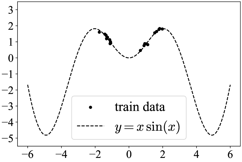
We employed the approximate entropy (3.2) for variational inference to a BNN whose posterior was modeled by the Gaussian mixture, which we call BNN-GM in the following. We conducted the toy 11 D regression task [He et al., 2020] to observe the uncertainty estimation capability of the BNN-GM. In particular, we observed that the BNN-GM could capture larger uncertainty than the deep ensemble [Lakshminarayanan et al., 2017]. The task was to learn a curve y=xsin(x)y=x\sin(x) from a training dataset that consisted of 2020 points sampled from a noised curve y=xsin(x)+εy=x\sin(x)+\varepsilon, ε𝒩(0,0.12)\varepsilon\sim\mathcal{N}(0,0.1^{2}). Refer to Appendix C.3 for the detail of implementations. We compared the BNN-GM with the deep ensemble of DNNs, the BNN with the single unimodal Gaussian, and the deep ensemble of BNNs with the single unimodal Gaussian, see Figure 4.

From the result in Figure 4, we can observe the following. First, every method can represent uncertainty on the area where train data do not exist. However, the BNN with a single unimodal Gaussian can represent smaller uncertainty than other methods (see around x=0x=0). Second, as increasing the number of components, the BNN-GM can represent larger uncertainty than the deep ensemble of DNNs or BNNs. Therefore, there is a qualitative difference in uncertainty estimation between BNN-GMs and deep ensembles. Finally, the BNN-GM of 10 components has weak learners with small mixture coefficients. We suppose that this phenomenon is caused by the entropy regularization for the Gaussian mixture. Note that we do not claim the superiority of BNN-GMs to deep ensembles.

Refer to caption

(a)  Dataset

Refer to caption

(b)  Deep ensemble of 5 DNNs

Refer to caption

(c)  Deep ensemble of 10 DNNs

Refer to caption

(d)  BNN (single Gaussian)

Refer to caption

(e)  BNN-GM of 5 components

Refer to caption

(f)  BNN-GM of 10 components

Refer to caption

(g)  Deep ensemble of 5 BNNs

Refer to caption

(h)  Deep ensemble of 10 BNNs

Figure 4: Uncertainty estimation on the toy 11D regression task. Each line indicates one component of the ensemble or mixture, and the filled region indicates the mean value of the prediction with the standard deviation×(±2)\times(\pm 2). As for BNN-GMs, the stronger the color intensity of the line, the larger the mixture coefficients of the model.

C.3 Details of experiment

We give a detailed explanation for the toy 11D regression experiment in Appendix C.2. The task is to learn a curve y=xsin(x)y=x\sin(x) from a training dataset that consists of 2020 points sampled from the noised curve y=xsin(x)+εy=x\sin(x)+\varepsilon, ε𝒩(0,0.12)\varepsilon\sim\mathcal{N}(0,0.1^{2}), see Figure 4. To obtain the regression model of the curve, we used the neural network model as the base model that had two hidden layers and 88 hidden units in each layer with erf activation. Regarding the Bayes inference for the BNN-GM, we modeled the prior as 𝒩(0,σw)\mathcal{N}(0,\sigma_{w}) and the variational family as the Gaussian mixture. Furthermore, we chose the likelihood function as the Gaussian distribution:

p(y|f(x;w))=𝒩(f(x;w),σy).\displaystyle p(y|f(x;w))=\mathcal{N}(f(x;w),\sigma_{y}).

Then, we performed the SGVB method based on the proposed ELBO (C.5), where the batch size was equal to the dataset size. Hyperparameters were as follows: epochs =100=100, learning rate =0.05=0.05, σw=106\sigma_{w}=10^{6}, σy=102\sigma_{y}=10^{-2}.