The WaZP galaxy cluster sample of the Dark Energy Survey Year 1
Abstract
We present a new (2+1)D galaxy cluster finder based on photometric redshifts called Wavelet Z Photometric (WaZP) applied to DES first year (Y1A1) data. The results are compared to clusters detected by the South Pole Telescope (SPT) survey and the redMaPPer cluster finder, the latter based on the same photometric data. WaZP searches for clusters in wavelet-based density maps of galaxies selected in photometric redshift space without any assumption on the cluster galaxy populations. The comparison to other cluster samples was performed with a matching algorithm based on angular proximity and redshift difference of the clusters. It led to the development of a new approach to match two optical cluster samples, following an iterative approach to minimize incorrect associations. The WaZP cluster finder applied to DES Y1A1 galaxy survey (1,511.13 deg2 up to mag) led to the detection of 60,547 galaxy clusters with redshifts and richness . Considering the overlapping regions and redshift ranges between the DES Y1A1 and SPT cluster surveys, all SZ based SPT clusters are recovered by the WaZP sample. The comparison between WaZP and redMaPPer cluster samples showed an excellent overall agreement for clusters with richness ( for redMaPPer) greater than 25 (20), with 95% recovery on both directions. Based on the cluster cross-match we explore the relative fragmentation of the two cluster samples and investigate the possible signatures of unmatched clusters.
keywords:
Galaxies: clusters: general – Galaxies: distances and redshifts – Methods: data analysis – Surveys1 Introduction
The abundance and clustering properties of galaxy clusters have been shown to be powerful probes to constrain cosmological models, provided that their astrophysical properties are well characterized and linked to theoretical predictions (e.g., Lima & Hu, 2005; Vikhlinin et al., 2009; Mantz et al., 2010; Benson et al., 2013; Weinberg et al., 2013; Planck Collaboration et al., 2016; DES Collaboration et al., 2020).
Galaxy clusters can be detected from X-ray observations (Kim et al. 2007; Lloyd-Davies et al. 2011; Adami et al. 2018) and from the Sunyaev-Zel’dovich (SZ) effect (Bleem et al., 2015), but on-going and future large photometric surveys constitute a very promising approach to build large controlled galaxy cluster samples for both cosmological and astrophysical studies. These include the Kilo Degree Survey (KIDS, de Jong et al. 2013), the Dark Energy Survey (DES, The Dark Energy Survey Collaboration Flaugher 2005), Pan-STARRS (Kaiser et al., 2002), the Legacy Survey of Space and Time (LSST, LSST Science Collaboration et al. 2009) and the European Space Agency Cosmic Vision mission (Euclid, Laureijs et al. 2011).
However, detecting and characterizing clusters through their galaxy component remains a nontrivial task, especially when considering lower mass or higher redshift clusters. One has to distinguish between gravitationally bound groups of galaxies and projection effects due to the underlying large scale distribution of galaxies. Projection effects not only impact detection, but also several fundamental properties of detected clusters, such as centering, redshift, and mass proxy (e.g., cluster richness).
Many automated algorithms were developed in the last three decades to overcome these difficulties. Automatic optical cluster finders can generally be described as algorithms searching for cluster scale galaxy overdensities. Galaxies are first filtered (or weighted) following prescriptions to increase the detection contrast relative to background galaxies. The main techniques used for searching galaxy overdensities include kernel smoothing (e.g., Shectman, 1985; Lumsden et al., 1992; Adami et al., 2010; Gladders & Yee, 2000), Friends-of-Friends (e.g., Botzler et al., 2004; Trevese et al., 2007; Wen et al., 2012) or Voronoi tesselation (e.g., Ramella et al., 1999; Soares-Santos et al., 2011). These techniques have been applied to galaxy catalogs that are usually previously filtered in one or several dimensions (e.g., magnitudes, colors, or photometric redshifts). More sophisticated approaches assume an underlying cluster model (e.g., density profile, luminosity function, color content) and identify clusters in likelihood maps based on matched filter techniques (e.g., Postman et al., 1996; Olsen et al., 1999; Koester et al., 2007; Olsen et al., 2008; Rykoff et al., 2014, 2016; Bellagamba et al., 2018).
A typical assumption of optical cluster finders is to consider the presence of a red sequence of galaxies (Gladders & Yee, 2000; Koester et al., 2007; Hao et al., 2010; Murphy et al., 2012). In low redshift clusters, the most luminous galaxies define a tight sequence in the color-magnitude diagram, the so-called "E/S0 ridge line", or "red sequence". Red sequence galaxies have very uniform colors and are among the reddest galaxies at a given redshift. Because of the strong 4000 Åbreak in their rest-frame spectra, their color is tightly correlated with redshift and can be used to estimate cluster redshifts. This feature has been observed in rich clusters up to (e.g., Mei et al., 2009; George et al., 2011; Wetzel et al., 2013; Strazzullo et al., 2019). However, some galaxy clusters observed at high redshifts can display appreciable star formation, even in cluster cores (e.g., Brodwin et al., 2013), weakening the red sequence.
Cluster finders such as maxBCG (Koester et al., 2007), redMaPPer (Rykoff et al., 2014, 2016) or RedGOLD (Licitra et al., 2016) rely on the red sequence for cluster detection and redshift estimate. In the context of recent surveys, cluster finders not based on the red sequence usually rely on photometric redshifts. An alternative based on the knee of the cluster luminosity function was also used in the context of surveys with a limited number of passbands (e.g., Postman et al., 1996; Olsen et al., 1999).
Even if current automated optical cluster finders are all able to identify rich clusters, evaluating their performances over broad ranges of masses and redshifts and deriving the selection function of the resulting cluster samples remain highly complex tasks. On the theoretical side, this requires the development of ever more realistic simulated galaxy catalogs. On the observational side, we need multiple surveys covering the same area at different frequency domains to detect clusters through a variety of signatures.
There is not a unique methodological framework to evaluate and compare the performances of optical cluster finders. A variety of approaches have been proposed, based either on mock galaxy catalogs (e.g., Euclid Collaboration et al. (2019) and references therein), or on real data, or even on a mix of the two approaches (e.g., Goto et al., 2002; Kim et al., 2002; Rykoff et al., 2014; Costanzi, M. & Rozo, E. et al., 2019).
Within simulations assumptions, simulation-driven methods provide a truth table useful for comparison, with clusters embedded in realistic large scale structures. These methods also offer a direct link between galaxy clusters and dark matter halos. However, they rely on sophisticated modeling that so far does not fully reproduce all observed galaxy properties, specially at high redshift (e.g., DeRose et al., 2019). In addition to this fundamental problem, mock catalogs do not usually reproduce the variety and complexity of defects occurring in observed images and introduced at the stage of source extraction and classification. DES has recently started to deal with this using the Balrog algorithm (Suchyta et al., 2016), which embeds simulations into real data and should accompany future releases.
Addressing the cluster selection function based on real data is necessarily limited by the absence of an absolute reference to confront the results of any cluster finder. Nonetheless, useful information can be extracted from the cross-match of a given optical cluster sample with detections based on different tracers that do not suffer from the same projection effects (e.g., Saro et al., 2015) A better understanding of the galaxy cluster selection function can also be improved from cross-matching samples from different optical cluster finders. The resulting samples may differ not only due the different adopted physical assumptions but also due to the details of cluster finder implementation (Ascaso et al., 2017; Aguena & Lima, 2018), or even the way the algorithms deal with specific features of real data (e.g. noise, missing data, star/galaxy separation, etc.).
DES has produced galaxy cluster samples with the redMaPPer algorithm which were published in Rykoff et al. (2016) and McClintock, T. & Varga, T. N. et al. (2019), based on DES Science Verification and DES-Y1 data releases, respectively. These samples led to several studies focusing on the mass-richness relation (Melchior et al. 2015; Saro et al. 2015; Zhang et al. 2016; Palmese et al. 2016; Saro et al. 2017; Melchior, P. & Gruen, D. et al. 2017; Pereira et al. 2018; McClintock, T. & Varga, T. N. et al. 2019; Bleem et al. 2020; Pereira et al. 2020). Complementary analyses were also performed on cluster luminosity function (Zhang et al., 2019b), baryon content (Chiu et al., 2018), and cluster miscentering relative to X-ray detections (Zhang et al., 2019a). These clusters were also used for the detection of voids (Pollina et al., 2019). Most of these studies contribute to the work on cosmological constraints using DES first year release redMaPPer clusters (DES Collaboration et al., 2020).
In this paper, we present the Wavelet Z Photometric (WaZP) cluster finder and apply it to DES-Y1 data. WaZP is an optical cluster finder designed to detect clusters based mainly on the spatial clustering of galaxies using photometric redshift information. The primary motivation for developing WaZP is to limit assumptions on the properties of cluster galaxies such as the presence of a red sequence, the shape of their luminosity function or radial profile, assumptions that may impact cluster detection, in particular at high redshift or at lower mass regime.
Here, the WaZP DES-Y1 sample is compared to cluster samples obtained from the SPT survey based on the SZ effect and those obtained by the redMaPPer cluster finder on the same DES-Y1 data set. The first comparison allows to test how well the WaZP algorithm recovers the massive clusters detected by the SPT. The second comparison, for which the two samples have similar cluster densities, gives insights on the relative completnesses of the two optical cluster samples, and on the derived properties of the common detections. Variations may occur in the samples due to the different assumptions made in terms of cluster modelling. They may also occur due to different uses of the underlying galaxy dataset as the WaZP algorithm uses magnitude information from all bands through photometric redshifts and -band as a reference band, whereas redMaPPer uses combinations of band pairs (colors) to select likely red sequence galaxies and -band as a reference. Considered survey coverage can therefore be slightly different with one approach or the other. Depth variability in all bands will also impact differently cluster detection with each algorithm. While the comparisons performed here provide a valuable heuristic approach to partly qualify the cluster samples, a complete evaluation of the WaZP sample requires to address a quantitative assessment of its purity, a work that will be presented in a companion paper based on mock galaxy catalogs.
The present paper is organized as follows. In Section 2, we describe the DES Y1 data used in our analysis. In Section 3, we describe the main properties of the WaZP cluster finder. In Section 4, we present our main results on DES-Y1 data. In Section 5 we matched the derived WaZP cluster samples to the SZ sample and to the redMaPPer sample obtained from DES-Y1 data. Finally, in Section 6 we analyze the properties of the catalog, and discuss the differences between our catalog and the others compared in Section 5.
Throughout this work, we fix cosmological parameters from the Planck results (Planck Collaboration et al., 2016) for a flat CDM model with and km s-1 Mpc-1.
2 Data
The DES is an imaging survey covering 5,000 deg2 in 5 bands ( ) (e.g., Flaugher, 2005; Diehl et al., 2016; Dark Energy Survey Collaboration et al., 2016). In this paper, we use the DES Year 1 data release, which has been extensively studied by the DES collaboration (e.g., Troxel et al., 2018; Shipp et al., 2018). The DES built the Dark Energy Camera (DECam, Flaugher et al., 2015) with a field of view diameter of 2.2 deg covered by 520 Megapixels distributed on a mosaic of 62 CCDs that are extra sensitive on the red part of the electromagnetic spectrum, enhancing its capability of observing high redshift galaxies. DECam is installed on CTIO 4-meter Blanco telescope prime focus, and its observations follow a strategy that optimizes pointings based on properties like weather and moon phase (Neilsen et al., 2019). The images are reduced and calibrated by the DES Data Management (DESDM) team at the National Center for Supercomputing Applications (NCSA). The DESDM pipeline includes the reduction of single-exposure images, their co-addition into deeper images, source extraction and calibration, all resulting in the creation of the main scientific catalog (Morganson et al., 2018).
The DES Year 1 Annual Release (Y1A1, Abbott et al., 2018) co-added catalog used in this analysis covers a total area of 1,520 deg2, split into two main wide regions. One of them has an area of 140 deg2 overlapping the SDSS Stripe 82 area (Aihara et al., 2011). The other part has an area of 1,380 deg2 overlapping the South Pole Telescope footprint (SPT, Carlstrom et al., 2011). In the following, we will refer to these two regions as Y1-S82 and Y1-SPT, respectively. They were observed with three to four exposures in each filter (Drlica-Wagner et al., 2018).
In addition to catalogs, we also use ancillary maps to track defects and foreground objects (e.g., bright stars, very bright galaxies, and globular clusters) all over DES footprint. The resulting coverage map is represented by a detection fraction map, where pixels have values of area fraction from 0 to 1. We also use systematic maps to track observing conditions across the footprint, such as number of exposures, seeing, and airmass (Leistedt et al., 2016). These maps are combined to produce depth maps based on galaxy magnitude limits, as described in Rykoff et al. (2015). All maps are recorded in Healpix format (nside = 4096) (Górski et al., 2005).
The Y1A1 coadd catalog and maps produced by DES DM were transferred to the Laboratório Interinstitucional de e-Astronomia (LIneA)111http://www.linea.gov.br and ingested into the database associated to the DES Science Portal (henceforth, the Portal) as described in Fausti Neto et al. (2018). We used the Portal infrastructure to create a galaxy Value Added Catalog (VAC) tailored for galaxy cluster search based on photometric redshift. The creation of the galaxy VAC includes: computation of photometric redshifts, star-galaxy classification, and pruning regions and objects to produce a clean galaxy catalog with well controlled levels of completeness and homogeneity. Along with the VAC, a final footprint map in Healpix format is created, reflecting the selection and pruning applied to this VAC.
The computation of photometric redshifts relies on the machine-learning algorithm DNF (Directional Neightbourhood Fitting, De Vicente et al. 2016), operated in Euclidean Neighborhood Fitting (ENF) mode since tests using DES Y1 data have shown that ENF mode is considerably faster, while providing similar results as in DNF mode. DNF uses as input observables SExtractor MAG_AUTO magnitudes (Bertin & Arnouts, 1996). DNF was trained with a large sample of spectroscopic redshifts extracted from a compilation of 29 public surveys intercepting the DES footprint. Quality flags of all surveys are brought to a common standard following OzDES approach (Yuan et al., 2015). As described in Gschwend et al. (2018), sources with flags 0 and 1 have unknown redshift, flag 2 redshifts are not reliable, flag 3 redshift reliability is above 90% confidence, and flag 4 is attributed to a trusted redshift (over 99% confidence). The DES photometric catalog is matched to this spectroscopic redshift sample with a 1.0 arcsec search radius and down to mag, producing a catalog of 101,971 galaxies with a mean redshift of 0.63, and covering the redshift range . Although color and magnitude distributions of this spectroscopic sample differ from the global photometric set under study, we stress that it does cover the same color-magnitude ranges with the exception of faint low redshift galaxies (typically magnitudes fainter than 19 and redshifts below 0.15). The spectro-photometric catalog is then randomly split into a training and a validation sets. Details about all the steps carried out to compute photometric redshifts in the DES Science Portal for Y1A1 data are described in Gschwend et al. (2018).
Star-galaxy classification follows a morphological prescription developed within the DES consortium called MODEST, described by equations (3) and (4) of Sevilla-Noarbe et al. (2018). It mainly depends on the SExtractor SPREAD_MODEL (Desai et al., 2012; Bouy et al., 2013) and its error, assessing how extended is the source to the local PSF. Note that this classification is based on the DES -band and extends to the faintest sources.
Based on bad regions maps (Drlica-Wagner et al., 2018), areas around bright stars, bleed trails, bright foreground galaxies, or globular clusters (from Harris, 2010) are removed from the footprint. Pixels with an effective coverage 0.1 are discarded from our analysis. We also exclude regions not covered simultaneously by bands with a minimum of 90s total exposure time. Besides region-based filtering, we also discard individual sources based on SExtractor FLAGS (only sources with FLAGS 3 are kept), apply a magnitude cut (), and color cuts (; ; ).
Depth maps, defined here as 10 limiting magnitude maps, were built following the method described in Rykoff et al. 2015. These maps correspond to the limit where the flux is at least 10 times its variance , computed from the magnitude errors. This definition assures a galaxy completeness larger than 90%. Figure 1 shows what survey area fraction is covered at a given 10 -band limiting magnitude (the -band being the reference band in this work). The whole survey is at least as deep as and shallower than with half of the survey area reaching . In Figure 2 we compare galaxy number counts for Y1-S82 and Y1-SPT with number counts from Arnouts et al. (2001) and Capak et al. (2007) as compiled by Nigel Metcalfe222http://astro.dur.ac.uk/ nm/pubhtml/counts/counts.html. The surveys used for comparison are deeper than our own, and number counts are comparable through a wide range of magnitudes up to mag, beyond which we observe an increasing deficit of galaxies, consistent with the median depth of the survey.


Based on the survey depth shown above, the present analysis considers galaxies down to a limiting magnitude (98% of the survey area). The resulting galaxy VACs for Y1-S82 and Y1-SPT contain, respectively, 4,721,380 and 45,206,403 galaxies, in a total of 49,927,783 galaxies covering 1,511.13 deg2. Both regions have similar galaxy number densities and mean photometric redshift (Table 1).
Figure 3 presents the projected galaxy distribution of Y1-S82 (top) and Y1-SPT (bottom)333These were produced with skymapper by Peter Melchior. The distributions are fairly uniform and galaxy densities comparable. Holes caused by masking and dents on the footprint caused by unobserved regions can be seen in both regions.
Normalized photometric redshift distributions are shown in Figure 4 for both regioggns. Our magnitude cut leads to a mean in both cases and very similar distributions. They both suffer from a counts drop around 0.4 due to the lack of the -band. This can also be seen in the left panel of Figure 5 where photometric redshifts are compared to spectroscopic redshifts for a validation sample of 50,476 galaxies built during DNF processing. There is an excellent correlation between spectroscopic and photometric redshifts; however, galaxies around 0.3 show a very large scatter, especially towards higher values of . This can also be seen in the right panel of Figure 5, where we assessed the global quality of the photometric redshifts by characterizing the average bias and standard deviation of . These points will be examined in detail in sections 4 and 6.


| Region | Galaxies | Area | Density | Mean |
|---|---|---|---|---|
| (deg2) | (Gal./arcmin2) | photo-z | ||
| Y1-S82 | 4,721,380 | 143.66 | 9.13 | 0.65 |
| Y1-SPT | 45,206,403 | 1,387.47 | 9.05 | 0.63 |


3 The WaZP cluster finder algorithm
The Wavelet Z-Photometric (WaZP) cluster finder is designed to detect galaxy clusters from multi-wavelength optical imaging galaxy surveys. It searches for projected galaxy overdensities in photometric redshift space without any assumption on the red sequence. In a nutshell, WaZP first slices the galaxy catalog in photometric redshift space, and then generates smooth wavelet-based density maps for each slice where peaks are extracted (see Figure 6). These overdensity peaks are then merged to create a unique list of clusters and associated galaxy members. Hereafter, these various steps are described in detail.

-
1.
Slicing in photometric redshifts. By photometric redshift slices, we mean here the photometric redshift support over which individual galaxy redshift PDF’s are integrated around a given redshift of interest. Therefore, at a given considered redshift, galaxies are weighted by that quantity. These weights are used to build density maps at different redshifts or estimate richnesses as described in the next steps.
The adopted strategy to define photometric redshift slices is based on the statistical comparison of the "best-estimate" discrete photometric redshifts (taken here as the mean of the galaxy redshift PDF) and corresponding spectroscopic redshifts if available. Based on available spectroscopic samples, the mean bias and scatter of photometric redshifts () relative to spectroscopic redshifts () were derived. Following the standard way to evaluate the performance of photometric redshifts (e.g., Ilbert et al., 2006), we computed statistics of as a function of both and . The location and width of a slice is then built in such a way that it includes 95% of the galaxies of a given spectroscopic redshift. The separation between two slices corresponds to a fourth of their width assuring a sufficient overlap to avoid missing clusters being between two consecutive slices.
-
2.
Generation of galaxy number density maps. WaZP does not consider photometric redshifts as discrete values. Instead, it operates with redshift PDF’s when provided, or generates them from the errors provided by the chosen photometric redshift algorithm. In each one of the slices defined above, galaxies are weighted by the integral of their redshift PDF over that slice. The resulting weighted RA-Dec distribution is then pixelized on a grid with a step of physical size 1/16th of a Mpc. This image is finally filtered using the wavelet task MR_FILTER from the multi-resolution package MR/1 (Starck et al., 1998). This task incorporates a statistically rigorous treatment of the Poisson noise, which allows us to keep significant structures in the desired scale range. Here we select structures with scales in the range Mpc, typical of cluster scales, and apply a 3 iterative multi-resolution thresholding with a B-spline wavelet transform.
-
3.
Extraction of peaks. The smooth density maps obtained in the previous step are segmented, and in each object domain, one or more peaks are extracted. In the case of several peaks in one domain, depending on the distance between a peak and the closest saddle point, the peak can be merged or preserve its identity. Pixels of a domain are then distributed to peaks by proximity.
-
4.
Assessing peak significance The peak significance is chosen to be computed in a radius of kpc, a radius that encloses typical cluster cores (Adami et al., 1998). To perform background statistics, the survey is pixelized with pixel areas equal to . Any pixel intersecting a bad region or an edge is removed. Standard counts in cells are then applied to estimate the mean density () and standard deviation (). The significance, defined as , where is the total density of galaxies in a cylinder centered at the peak position, with a length that is the width of the redshift slice and an angular radius .
-
5.
Peak merging along the redshift direction. As slices overlap, one can expect clusters to be detected in several consecutive slices. To build the final list of clusters, peaks of consecutive slices are associated, and only the slice in which the system has maximum significance is kept. Note that two clusters can be deblended along the line of sight if their distance in redshift is larger than 2 where denotes here the 68th percentile of the distribution.
-
6.
Centering and cluster redshift. The cluster center is defined as the location of the density map peak. However, if the brightest cluster member is found within the first neighbouring pixels, then this galaxy marks the center. This leads to a maximum shift of 100 kpc from the peak location. Concerning the redshift, an initial value is derived as the mode of the sum of the galaxy redshift PDF’s within a 0.5 Mpc radius around the cluster center. This value is refined iteratively based on the membership probabilities described below.
-
7.
Assignment of membership probabilities. Membership probabilities () are computed following the prescription given in Castignani & Benoist (2016). In a nutshell, galaxies of the cluster field are piled up in a 3-dimensional grid (cluster-centric distance, magnitude, photometric redshift) where magnitudes and redshifts are included as probability distribution functions. The same is done for local background galaxies in (magnitude, photometric redshift) space. The local background galaxies are selected in a ring from 3 to 6 Mpc to the cluster center, whereas cluster field galaxies are selected within a 3 Mpc disk. The membership probability is the combination of the probability to be at the cluster redshift and the probability not to be a background galaxy. The final membership probability at a given cluster-centric distance, magnitude, and redshift is derived from the density ratio between the cluster field and the background field. Note that, as in Castignani & Benoist (2016), no parametric modelling is used for the radial density, nor for the luminosity function.
-
8.
Richness and radius The cluster richness and radius are estimated jointly. The richness is the sum of the membership probabilities within a radius that corresponds to an overdensity of 200 times the mean galaxy background number density (similar to Hansen et al. 2005). This is done considering galaxies, both in the field and in the cluster, down to a given fraction of luminosity. Practically, galaxies brighter than are counted, where is the characteristic magnitude marking the knee of the luminosity function and is a fixed quantity, chosen here to be 1.5. The adopted definition allows to produce "redshift independent richnesses", in the sense that the same cluster seen at two different redshifts would have the same richness. The evolution of the characteristic luminosity of the Luminosity Function can be described by a passively evolving population formed in a single burst (e.g., Lin et al., 2006). In this study, we derive from the passive evolution of a burst galaxy with a formation redshift taken from the PEGASE2 library (burst_sc86_zo.sed, Fioc & Rocca-Volmerange, 1997). It is calibrated using the value of () derived by Lin et al. (2006) from an observed cluster sample. The choice of is critical as it sets the redshift limit () of the final cluster sample through the relation , where is the survey apparent magnitude limit.
4 Application to DES-Y1 survey
4.1 Running WaZP cluster finder
As described in section 2, the DES-Y1 survey is split into two regions ("SPT" and "S82"), for which two galaxy VACs are produced to feed the WaZP pipeline. These catalogs are built based on the -band, chosen here as a reference band both for star-galaxy separation, and for defining apparent magnitude cuts. Given this selection, cluster detection was performed with the same setting independently from the position on the sky, assuming a sufficient homogeneity over the whole survey. This is an approximation as we have seen above that in some regions magnitude completeness limit can be lower by as much as 1 mag.
The redshift limit of the constructed WaZP sample is constrained by the depth of the survey reference band. It also depends on the adopted definition of the richness estimate and in particular, the adopted magnitude limit used to count galaxies entering the richness. We assume here that the same cluster, seen at two different redshifts, would get the same richness by counting its galaxies down to an apparent magnitude , where is a fixed quantity and is defined in section 3. This can be achieved as long as this quantity remains lower than the -band depth of the survey. In the present case, richnesses are chosen to be computed including galaxies down to .
Based on the above considerations, given that some regions are not deeper than , there is an upper redshift limit, , above which richnesses start to become incomplete depending on the survey location. At the limiting magnitude of the galaxy VAC, , which corresponds to a redshift limit , richnesses are complete within only 2% of the survey area. Based on the 10 -band survey depth map (section 2), we have derived a map indicating our local cluster at each position of the survey, that is reported in the WaZP cluster catalog. Detection is performed to slightly larger redshifts (), but for clusters that would be detected beyond their local , their galaxy luminosity function is not sampled homogeneously across redshifts and therefore richnesses for these clusters would require some correcting factor. In this paper, we are not introducing such a correction, and therefore richnesses are consistent over the whole survey only up to . As a lower redshift limit for cluster detection, we adopted in this paper the value .
Besides the considerations on redshift limits above, we also need to assess the global quality of our photometric redshifts and determine the photometric redshift slicing strategy on running WaZP. As can be seen in the right panel of Figure 5, the average bias remains relatively modest and the scatter roughly constant in the adopted redshift range. These properties should not prevent cluster detection in general. Note, however, that this point will be discussed in more details in section 6.
Operationally, the WaZP cluster finder runs on small sections of the sky. The LIneA Science Portal manages data tiling, launches the code on each tile on parallel cores and concatenates the final catalogs, both clusters and galaxy members. The data tiling consists in dividing the survey in overlapping rectangular tiles of typical area 20 deg2. The overlaps are set to assure a tiling independent cluster detection for clusters with redshifts larger than 0.05 that would fall at the intersection of two tiles.
4.2 The WaZP cluster catalog
The WaZP pipeline was run on the DES Y1-S82 and Y1-SPT regions defined above. This results in the detection of cluster candidates, not confirmed galaxy clusters. However, these candidates will be referred to as "WaZP clusters" throughout the paper for simplicity. For the combined sample, it led to the detection of 60,547 clusters in the redshift range to with richness , corresponding to densities of 40.47 and 39.45 clusters/deg2 for Y1-S82 and Y1-SPT respectively . If we restrict to a sample with more reliable redshifts and complete richenesses i. e. , we find 39,439 clusters, with a higher consistency in cluster densities with 26.25 and 25.71 clusters/deg2 for the two DES regions. This result supports strongly the high homogeneity over the sky of the galaxy VAC construction, including photometric redshift computation, as well as the subsequent cluster detection. This can also be seen in Figure 7 where the projected distribution of detected clusters on the sky is shown. A description of the WaZP cluster catalog is provided on LIneA’s website444https://www.linea.gov.br/catalogs/wazp/.


The ranges of richnesses and redshifts covered by WaZP clusters are shown in Figure 8. From the color coded SNR we can see that for a given richness, as expected, the SNR decreases with redshift. This is mainly due to the increasing scatter in the photometric redshifts leading to an increase of the mean background density of galaxies. We see that above redshift , the number of rich clusters start to diminish rapidly, and above there is only one cluster with richness greater than .

The redshift distribution of WaZP clusters is shown in Figure 9. The global bell shape of the counts looks as expected except for a sharp concentration of clusters at , similar to that observed on the galaxy photometric redshift distribution of Figure 4. This peak becomes more prominent for lower richness systems. In the next sections we investigate further the nature of this peak.

There are several ways to estimate the quality of the WaZP redshifts (). They can be compared to known cluster redshifts as shown in the next section, or, as done here, cluster members can be cross-matched with available spectroscopic galaxy samples. The adopted procedure here is to search for all galaxies with spectroscopic redshifts within 0.5 Mpc around each detected cluster and likely to be cluster members. We considered that a cluster could be associated with a spectroscopic redshift if at least 5 galaxies were found within a range of km/s. The selected velocity window is the one that maximizes the number of spectroscopic galaxies. The cluster spectroscopic redshift is then defined as the median of the redshifts in that window. We also associated a redshift in the case the central WaZP cluster galaxy has a spectroscopic redshift. This may lead to a few outliers but increases statistics by a factor of 10. Based on public spectroscopic surveys, 131 WaZP clusters covering the redshift range to could be associated a spectroscopic redshift with at least 5 concordant redshifts, and 1,859 clusters could be associated a spectroscopic redshift based on their central galaxy. In Figure 10, the comparison with WaZP redshifts is shown. Both spectroscopic redshift assignments led to the same statistical differences with WaZP redshifts: an average bias of 0.014 and scatter of 0.026.


Figure 11 shows the evolution of the volume density of clusters with redshift, with Poisson errorbars. We can see that the density for both Y1 regions agree with each other for both richness cuts.
5 Comparison to other cluster catalogs
In this section, we compare the WaZP Y1A1 clusters identified in the previous section to those derived by other methods covering the same region. A first comparison is made with clusters detected by the South Pole Telescope (SPT) survey via the Sunyaev-Zel’dovich (SZ) effect (Bleem et al., 2015). A second comparison is done with clusters detected by the redMaPPer optical cluster finder, based on the same photometric data but using an algorithm searching for overdensities of red sequence galaxies (Rykoff et al., 2014). These comparisons are based on matching clusters from two different catalogs. This is a complex operation that has led to a variety of proposed algorithms (e.g., Gerke et al., 2005; Knobel et al., 2009; Cucciati et al., 2010; Gerke et al., 2012; Euclid Collaboration et al., 2019). We point out that adopting one algorithm or another or using different configurations of the same may result in different cluster associations. In particular, when a given cluster can potentially be connected to several counterparts. As detailed below, we have experimented with several of these approaches and finally adopted a hybrid iterative procedure to optimally solve multiple matches. This appeared to be the only way to avoid having systems left unmatched due to a wrong matching of their obvious counterpart. Several such cases appeared in particular with interacting clusters for which richness rankings were reversed. The resulting pairing seems, from intensive visual inspection, optimal for addressing statistically the different properties of the commonly detected clusters (centering, redshift), and evaluating systems without any counterparts. In particular, our matching procedure allowed us to decrease the number of incorrect matches of rich clusters on each side significantly.
In this paper, we use a cylindrical matching where we require the angular distance of cluster centers to be smaller than some defined length (be it their respective radii or a fixed physical distance), and their redshift separation to be constrained by the typical redshift errors from both samples. In carrying out this comparison, some issues have to be considered. First, the cluster radius definition for each cluster sample may be different. Second, we must define the redshift window to be used. It should be large enough to take into consideration the errors in photometric redshift assigned to clusters in both samples. However, a large window may lead to an increased number of multiple matches that need to be resolved as discussed in more detail below. Finally, it is crucial to ensure that the projected area of overlap of the samples is properly taken into account. To do that, footprints of the samples are used to flag clusters falling outside the overlapping regions or near their edges. This flag is useful when unmatched clusters are near the edges, in which case they can be removed from the matching statistics.
As mentioned above, we compare the combined Y1-S82 and Y1-SPT clusters identified by WaZP with those in the SZ and redMaPPer samples. In the first case, we take the SZ sample as reference, treating the SZ clusters as true representatives of the underlying mass distribution and test how well these systems are recovered. In the redMaPPer case, we investigate the unmatched cases in both directions to understand the specificities or the possible limitations of each algorithm.
5.1 WaZP versus SPT clusters
The SZ sample (Bleem et al., 2015) covers an area of 2,500 deg2 (seen in bottom panel if Figure 9), within which 516 clusters (out of 677 candidates) were detected with signal-to-noise above 4.5. In Bleem et al. 2015, it is stated that the catalog is highly complete for and . It is also mentioned that there were a number of optical followups to confirm these clusters. Therefore, this catalog will be utilized to validate the detectability of WaZP regarding massive clusters. We only use the 331 SZ clusters that have information on mass and redshift, and are located within the overlap with DES (external envelope of the DES Y1-SPT region). We should stress that the redshifts assigned to SZ clusters from Bocquet et al. (2019) are both spectroscopic (106) and photometric (225).
We considered a one-way match, taking SZ clusters as reference and we looked for WaZP clusters falling within SPT clusters radii. The adopted radius is , the radius where the average cluster overdensity is 200 times the critical density, i.e., . It was computed from the available values of and converted to an angular radius using Planck Collaboration et al. (2016) cosmology. Here, , where is the comoving angular diameter distance to the cluster redshift . For a match to happen, the redshift separation also has to fall within the interval defined by the combined redshift errors. This interval was defined as where is the sum of redshift errors provided by the two catalogs. The resulting matching cylinder is quite large in order to account for possible centering offsets between the two wavelength domains and large redshift discrepancies. The statistical comparison, a posteriori, of the differences in centering and redshifts of the matched systems, allows us to evaluate the adopted matching criteria.
Applying this method to the SZ and WaZP samples, we find that 292 SZ clusters (out of 331) have at least one WaZP counterpart. Among these, 141 have only one candidate for matching, while the rest have a multiplicity function as shown in Figure 12. The large fraction of multiple matches is not surprising considering the very different selection functions of the two samples, their relative densities and the adopted matching criteria. The multiple WaZP matches were resolved by choosing the richest associated counterpart.

Out of the 39 unmatched SZ clusters, 12 are located near the WaZP footprint edges and 27 have redshifts beyond , where WaZP cluster finder reaches its expected limit of completeness for DES-Y1 (9 of those have , and are completely beyond WaZP reach). There was one unmatched SZ cluster (SPT-CLJ2218-5532) with , just above the redshift limit for WaZP clusters with complete richnesses. However, the local at this cluster position is and, upon visual inspection, we found no clear visible optical counterpart.
In Figure 13, we show the characteristics of the matching for three mass bins, both in terms of angular separation (left panel) and redshift separation (right panel). The average distance of WaZP-SZ centers is , with 80% of clusters within and 95% within . If we consider the different mass bins in the figure, there is a small systematic improvement on for higher masses (, and respectively), even though there is only clusters per mass bin. We also see that there is a reasonable agreement in redshift, with 79% of matches within the average redshift uncertainties of the clusters (gray shaded region). There is also a slight improvement on redshift scatter and bias was we look at higher mass bins.
We also compare the photometric estimates of WaZP redshifts with those assigned to SZ clusters. As 93 of the matched SZ clusters have been assigned a spectroscopic redshift (Bocquet et al., 2019), we can assess the accuracy of the estimated WaZP redshifts. Figure 14 shows the distribution of redshift separations (left) and relation of redshifts (right), splitting the SZ cluster redshifts into spectroscopic and photometric subsamples. As can be seen, WaZP redshifts show a good agreement with SZ spectroscopic redshifts and some residual relative bias when compared with SZ photometric redshifts. A quantitative description is provided in table 2, which gives in column (1) the type of sample; in column (2) the number of clusters and in columns (3) and (4) the bias and the scatter, defined as the mean and standard deviation of , and column (5) is the combined redshift errors . When compared to photometric redshifts, we measure a relative bias of and a scatter , a value similar to the combined redshift error 0.030. However, when comparing to SZ clusters with spectroscopic redshifts, WaZP redshifts are almost unbiased (bias ), and show a significantly lower scatter (, also compatible with the combined errors 0.015), corresponding to roughly half the average galaxy photometric redshift scatter. It is interesting to note that in all samples, the scatter was very close to the redshifts uncertainties, even though the matching conditions only imposed a redshift difference of three times the errors. From the right panel of Figure 14, it can also be seen that the moderate average bias is actually mainly due to low redshift clusters ().


| Sample | N | bias | scatter | errors |
|---|---|---|---|---|
| All redshifts | 292 | 0.012 | 0.026 | 0.025 |
| Phot z only | 200 | 0.015 | 0.029 | 0.030 |
| Spec z only | 92 | 0.007 | 0.017 | 0.015 |
5.2 WaZP versus redMaPPer
In this paper we also match WaZP clusters with those detected by the redMaPPer algorithm. Here we use the redMaPPer volume limited cluster catalog of DES-Y1 presented in McClintock, T. & Varga, T. N. et al. (2019) which consists of 83,238 clusters with richness 5 found in the Y1-SPT and Y1-S82 regions (seen in Figure 9) over the redshift range 0.1-0.95. This volume limited catalog considers clusters for which the local -band depth assures a complete galaxy catalog down to the adopted magnitude limit of the richness definition. The variable -band depth translates into a variable redshift limit () map that characterizes the cluster sample. When evaluating the recovery rates of clusters at high redshifts, we also consider the full redMaPPer cluster catalog over the same region, defined by a constant 0.95 and a richness threshold of 20.
5.2.1 Differences in the detection algorithms
redMaPPer is an optical cluster finder based on the detection of spatial overdensities of red sequence galaxies (Rykoff et al., 2016). Although WaZP does not make any assumption relative to the cluster galaxy population when searching for galaxy overdensities, we do expect these two algorithms to yield similar samples up to redshifts 0.7, at least when considering the richest systems. However, a number of differences can be expected in the cluster characterization for several reasons. First, as it was stressed above, galaxies used for searching for overdensities are not selected in the same way. redMaPPer selects them based on colors whereas WaZP selects them based on redshifts. Second, the two algorithms differ in defining cluster centers. In the case of redMaPPer centers are associated to a bright galaxy with some probability of being a central galaxy, whereas WaZP defines the center as a centroid. Note however, that, as described above, WaZP moves the center to the brightest cluster member position if its distance is less than 100 kpc, which happens here for 68% of the WaZP clusters. Third, redMaPPer redshifts are assigned based on an empirical modelling of red sequence colors, whereas WaZP assigns redshifts based on a concentration in photometric redshift space including all galaxy types at the cluster location. Finally, we also expect differences on how each cluster finder performs in terms of deblending, or in terms of fragmentation and over-merging.
The above effects make the matching between the two samples non-trivial, since the key elements to perform a proximity matching, like centering and redshift, can have distinct behavior, that may not lead to a unique solution. Despite its complexity, it should be able to provide us with a measure of the statistical consistency of the two catalogs. It should also help us infer a lower limit for centering uncertainty, as both cluster finders have optical centering estimations. Finally, by carefully dealing with footprint coverage and edge effects, it should allow us to identify a number of missing systems and provide feedback on the respective selection functions, on possible ways to improve cluster detection algorithms and improve aspects of the construction of the underlying galaxy catalog.
5.2.2 Matching procedure
In contrast to what was done in the comparison between WaZP and SPT clusters, here, each cluster sample is considered as a reference to the other. Therefore, not only we consider a one-way match using redMaPPer as a reference (redMaPPer-matched), but we also analyse the case where WaZP (WaZP-matched) is the reference catalog. These one-way matches are used to investigate the fraction of missed detections. In addition to the one-way matches, in order to estimate differences in cluster properties (e.g., centering, redshift, richnesses), we also carry out a two-way (unique) match, for which it is required that both one-way matches point to the same cluster.
We recall that the cluster matching is performed within a specified redshift window. Following what is done in section 5.1 when matching with SZ clusters, this window was first defined considering the sum of the redshift errors provided for each cluster in the different samples. However, while visually inspecting a sample of unmatched systems, it was noticed that for relatively low redshifts (), obvious pairs (i.e., sharing exactly the same center without any other overdensity on the line of sight) were not associated due to large redshift discrepancies. This fact is not surprising due to the systematic errors in photometric redshifts occurring at low redshifts. In order to take this effect into account, we used an empirical approach to define the redshift window for matching. We first matched systems by angular center proximity only, without a redshift window, but imposing the center angular positions to be closer than 0.05 Mpc, computed at the largest redshift of the cluster pair. The clusters were ranked by richness, and when multiple candidates were found (about 10% of the time for WaZP clusters and 24% for redMaPPer), the richest candidate was selected. As judged by eye inspection, with this criterion, most matches refer to the same system.
Figure 15 presents the resulting relation between redshifts for WaZP and redMaPPer matched clusters. As can be seen, this relation shows some deviations from a linear relation, in particular at WaZP redshift , where redshifts are distributed from 0.2 to 0.5, so a large scatter. This issue is discussed in more details in the following section. Based on this plot, we defined a new redshift window to carry out the matching, which corresponds to the union of the 99 percentile of the redshift differences using redMaPPer as reference (as it is covering a smaller redshift baseline) and a scatter.

Matching the catalogs by considering the resulting large redshift window combined to larger angular radii than in figure 15 unavoidably leads to a large fraction of multiple associations. Resolving these multiples by selecting the richest available system on both sides resulted in many false matches. An emblematic case that appeared several times in our visual inspections, is the case of interacting clusters of similar richnesses. Both cluster finders would detect the two components but not necessarily with the same richness ranking. In that case the matching could lead to one mis-match and one unmatched cluster, or more mis-matches due to a cascade effect. However, in the case of absence of an interacting system or if neighbouring systems are much poorer, the richness ranking is more adequate.
We found that for maximizing the number of correct associations, the best option is to go beyond a single matching rule. Therefore, we decided to perform the matching following a several steps process where the most unambiguous pairs are matched first and then proceed to the rest of the list. The steps are detailed below.
It was determined empirically that a four-step process is optimal, where, at each step, the matching would only be performed on clusters not previously matched. In the first step, we do not consider the clusters’ redshift, and match all clusters that have the exact same centering (which happens when the two cluster finders are centered on the same galaxy). By construction, each one way match finds the same corresponding pairs, therefore all cluster pairs found here will also be a match in the two way matching. This led to a total of 15,534 matched clusters. In the second step, remaining clusters are matched within an angular distance of kpc (computed at the lowest redshift of the pair) from each other, and a redshift difference less than (computed from Figure 15). When more than one candidate is found, the richest one is considered to be the correct match. This step also results in having the same number of matched clusters for both one way matches, adding an extra 6,431 matched clusters in each catalog. The third step expands on the second one with a window, leading to additional 3,783 matches in each catalog. In the last step, we match the remaining clusters with the empirical redshift window shown in Figure 15 and use the radius provided by each cluster finder as a parameter for angular distance. Here, the matching is not symmetric and results in another 4,915 and 3,027 matched clusters for redMaPPer and WaZP respectively. Hence, we obtained a total of 30,663 one-way matches for redMaPPer and and 28,775 for WaZP. We note that, in this four-step matching, if we do not remove matched clusters at each step and allow for multiple matches, we obtain 32,467 redMaPPer matched clusters and 33,498 WaZP matched clusters.
Finally, two-way matches are obtained when the two one-way matches point to each other. This results in 28,621 redMaPPer-WaZP cross-matched clusters.
5.2.3 Comparison of the matched clusters
We start by comparing the individual properties of the matched clusters (i. e. centering, redshift and richness). Cross-matched clusters (28,621 pairs) will be used in this evaluation, as a reliable one-to-one correspondence between clusters is required. Figure 16 shows the distribution of angular separation (left panel) and the redshift difference (right panel) of two-way matched clusters. As it can be seen, all matched clusters are well within the mean radius of the clusters (kpc), that was used in the last step of the matching. In 56% of the cases, clusters have the exact same center. Those occur when WaZP defines the same BCG as redMaPPer to be its center. The average distance of central position for the clusters that do not share the same center is of 86kpc, with 86% of matched clusters within 100kpc of each other and over 99% within 300kpc. The angular separation only shows a very weak tail beyond the typical cluster core radius. In addition, we note that the centering statistics do not seem to depend significantly on the richness.
Turning to the distribution of the redshift separations, we find that for the vast majority of pairs (), the redshift separation is well within one third of the redshift window used in the last step of the matching, which has an average size of . Additionally, we find over 75% of pairs with redshift separation within the combined uncertainty of the cluster redshifts (gray shaded region). We note, however, a small average redshift bias of (Table 3) exists between WaZP and redMaPPer , with redshifts derived by WaZP being on average slightly larger than redMaPPer redshifts. In Figure 17, redMaPPer and WaZP redshifts are compared, showing that the bias is mainly due to a significant fraction of clusters that were pushed to , an effect that is discussed in the next section. Additionally, we see on the right panel that this effect occurs mainly on poor () clusters. Overall, these results show that most matches are well within the ranges adopted in the matching procedure. It strongly supports the idea that we are detecting on average the same systems. We also note that the scatter is very similar to the combined redshift uncertainties in all richness limited samples (Table 3), and the biases are well within these values.
| bin | # clusters | |||
|---|---|---|---|---|
| All | 28,621 | 0.010 | 0.027 | 0.028 |
| 5-12 | 15,099 | 0.010 | 0.029 | 0.031 |
| 12-20 | 7,531 | 0.010 | 0.025 | 0.027 |
| 20-30 | 3,440 | 0.011 | 0.023 | 0.024 |
| 30-50 | 1,918 | 0.011 | 0.021 | 0.021 |
| 50-234 | 632 | 0.014 | 0.019 | 0.018 |


We now compare the values of richnesses as derived from the two algorithms. We do not expect them to be equal in average as they are derived with different definitions. redMaPPer richness () considers red sequence galaxies down to 0.2L∗ in the -band, whereas WaZP richness () considers all galaxies down to 0.25 in the -band. Moreover these quantities are not necessarily computed in the same angular radius. Despite these differences, we expect some correlation between these two richness estimates. To perform this comparison we restrict to two-way matched clusters with same centers and redshift offsets . We also considered clusters in the redshift range 0.1 - 0.6 in order to assure richnesses to be complete for both cluster finders. Figure 18 shows a strong correlation between the richnesses of the two cluster finders, with WaZP richnesses on average systematically larger than redMaPPer ones. To quantify the effect, we performed a linear fit in space. To do so, cluster richnesses were first sliced in and for each slice the mode of the smoothed distribution of computed. This procedure minimizes the effect from Malmquist bias when constraining the relation between richnesses. The fit of the resulting pairs led to the relation:
| (1) |
An independent comparison of the two estimated richnesses is based on the cluster density given a richness threshold. This is shown as the blue dashed line in Figure 18. Each point of this line provides the threshold in and in richnesses to obtain the same density in the two cluster samples, and is independent of any matching. It is remarkable that this measurement is very close to the mean relation between the two richness estimators. Another way to look at this is to compare directly the densities of the two cluster samples. In Figure 19, we compare WaZP and redMaPPer cluster densities considering clusters with redshifts in the range 0.1 - 0.6 and with richnesses above a given threshold, where the threshold in and are related following Eq. 1 (e.g. is equivalent to ). Cluster densities are very similar over a very wide range of richnesses. This result supports the idea that, on average, the ranking of the two cluster samples by their richness is similar.


5.2.4 Statistics of unmatched clusters
We now evaluate the recovery rates between catalogs. Our main goal in this section is to check if each cluster finder could have missed a detection, therefore we take a very conservative approach to label clusters as unmatched. In principle, these rates could be computed considering a two-way matching. However, in that case, if a cluster of the first sample appears to be fragmented in the second one, the extra cluster will be counted as not recovered. Here, we wish to separate the absence of a counterpart from fragmentation, which should be treated separately. Therefore, we defined the recovery rate as the fraction of clusters having one or more counterparts in the matched cluster sample. Obviously, the absence of a match does not exclude completely the existence of a counterpart. Some systems could suffer from a strong mis-centering, larger than tolerated by the matching criteria. Other systems could also suffer from edge effects that may occur at the periphery of the survey or close to a masked region within the survey. To minimize the latter, we do not consider unmatched clusters outside the intersection of the two cluster sample footprints (constructed as nside Healpix maps) or unmatched cluster located in edge pixels. In addition, as redMaPPer removes clusters with over 20% of their area masked, an equivalent consideration had to be made when looking for WaZP counter-parts. Hence, unmatched clusters whose cover fraction was less than 80% on the other catalog’s detection fraction footprint were also discarded from the analysis. These cover fractions were computed using the same weighted methodology as (Rykoff et al., 2014) considering the other catalog footprint. Although this is not a major contribution for the values of the recovery fraction of WaZP clusters, ignoring this effect leads to lower recovery close to the footprint edges and holes. It is also important to note that, because both catalogs have a footprint with a variation on at different locations, the computation of whether the cluster is inside the footprint or in a edge pixel and its cover fraction depends on the cluster position and redshift.
These cuts, based on the footprints and cover fraction, removed 16,283 and 18,737 redMaPPer and WaZP clusters without counterpart, respectively, from our recovery rate analysis. These clusters certainly contain information regarding each cluster finder selection function and limitations, however the study of these objects require a different analysis on a object-by-object case and will be done in a future work.
With these considerations, for one-way matching including the possibility of multiple associations, the recovery rate analysis is based on the total of 66,955 redMaPPer and 43,980 WaZP clusters with 32,467 and 33,498 matched respectively.
The recovery rate for each catalog as a function of redshift in different richness bins is shown in Figure 20. The left panel shows the fraction of redMaPPer clusters recovered by WaZP and the right panel the other way around. The gray shaded area is the redshift region where the redMaPPer (left panel) and WaZP (right panel) footprints decreases in size, with the dashed line being the median value of this footprint redshift limitation (i. e. where the area drops to 50% of the total footprint). The different shades correspond to the 95% and 100% percentiles of the distribution. We binned redMaPPer clusters into 5 samples, 2 bins for lower richness () clusters, that were not used for cosmological constraints (DES Collaboration et al., 2020), and 3 sample with higher richness. WaZP clusters were binned on the corresponding richness using our fit on Eq. 1. One can see that redMaPPer clusters with are mostly () recovered up to the WaZP redshift limit. Similarly, at the same level of richness (), we find that WaZP clusters are also recovered at more than up to the redMaPPer redshift limit of . We also note rapid increase in the recovery rate of clusters with richness in both cases. Considering the range, the overall recovery rate of redMaPPer clusters is 93.3%, 98.4%, 99.7% for bins (, and respectively). For WaZP clusters, similarly, we have 95.4%, 97.9% and 99.7% for bins (, and respectively). Major differences occur when considering clusters less rich than (). It is remarkable that even in the range 5 to 20 ( 5.6 to 25), clusters are still recovered at rates between 50 and 60%, depending on the redshift. The dotted vertical line corresponds to the minimum redshift of redMaPPer clusters (), hence the low recovery rate for WaZP clusters in the first redshift bin.
We note that the recovery rates reach 100% at high redshifts in both panels of Figure 20. This is an effect of the footprints variable redshift limit leading to smaller effective area as redshift increases, with only () of the redMaPPer (WaZP) area remaining at (). Consequently, at those redshifts, all unmatched clusters are removed from the analysis, resulting in an artificially perfect recovery. To obtain a more relevant WaZP recovery rate at high redshifts, we combined redMaPPer volume limited catalog () with the redMaPPer full catalog (uniform of and ) and matched it to the WaZP catalog using the procedure described above. These results are represented by the shaded lines in Figure 20. We see now that the redMaPPer recovery rate for clusters extends to higher redshifts. Comparing the WaZP recovery fraction to the matching with redMaPPer volume limited only, we have a general decrease at high redshifts. The lower recovery rate of clusters is directly correlated with poorer clusters () missing in the redMaPPer full catalog. Richer clusters () are affected by the scatter down of the richness relation between both cluster finders.
We conclude from this analysis that, statistically, rich systems are found by both cluster finders, independent of their redshifts, with very few individual differences that are investigated in the next section.
6 Discussion
We have shown that all SZ clusters with redshifts 0.76 intersecting our footprint are recovered by WaZP cluster finder applied on DES-Y1 data. We have also shown that more than 90% of clusters with richnesses above 20 detected by redMaPPer (or 25 by WaZP) are matched to those detected by WaZP (or by redMaPPer). In this section we compare some properties of the the two optical cluster samples. In particular, we explore differences such as redshift discrepancies, overmerging / fragmentation, and the reasons for unmatched systems on both sides.
6.1 Redshift discrepancies between WaZP and redMaPPer
Whereas the comparison of WaZP redshifts with spectroscopic redshifts assigned to SZ clusters (see table 2) showed moderate bias and small scatter, the comparison with redMaPPer clusters revealed stronger discrepancies. This is related to the fact that redMaPPer (and WaZP) clusters are on average much less massive than SPT clusters. This is confirmed if we restrict the cross match between WaZP and redMaPPer to richer clusters. In that case, as shown in the right panel of Figure 17, a reduced redshift bias and scatter is observed between the two samples.
The fraction of redshift outliers (defined by a redshift difference ) is less than 5% of our clusters, with 78% (82%) of them having (). These redshift outliers are mainly produced at . This also reflects on WaZP cluster number counts (Figure 9), that showed a peak at redshift 0.4 that becomes more prominent when considering the poorest clusters. From the same cluster number counts, a deficit of clusters at can also be noticed. These points support the idea that in the redshift range 0.15 - 0.35, WaZP detects on average the same clusters as redMaPPer but shifts a fraction of these to .
From global statistics of photometric redshifts, only moderate bias is measured (see right panel of Figure 5). However, this global bias includes galaxies of all magnitudes down to . In order to understand the shift in redshift of a fraction of WaZP clusters, one needs to investigate the photometric redshift bias at least as a function of both redshift and magnitude. This is what is shown in Figure 21. We binned our spectroscopic sample in -band magnitude and spectroscopic redshift and computed, for each bin with at least 100 galaxies, the median and standard deviation of . The amplitude of the photometric redshift bias is shown as a color code. In most regions of this diagram, the bias is moderate, consistent with the global bias. However, for redshifts between 0.15 and 0.35 and -band magnitudes fainter than , we find a strong bias that reaches values of 0.1-0.2.
The origin of this strong bias is two-folded. It is first due to the lack of -band and to the transition of the 4000Å break between and band at redshift . Second, it is due to the lack of faint () red galaxies at redshifts below in our spectroscopic training sample. We stress that for these faint, low-redshift and red galaxies, the bias may be even larger as it cannot be estimated properly. The consequence is that their photometric redshift is overestimated, pushed to redshifts where the training set samples better the same (magnitude, colors) space. This effect has already been stressed in several other studies (e.g., Figure 25 of Rykoff et al., 2016).
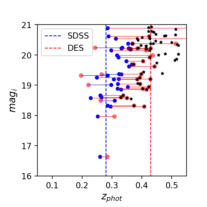
This statement can actually be tested by comparing how a DES redshift biased WaZP cluster is detected in the Sloan Digital Sky Survey, that is covered in bands in the overlapping Stripe 82 region. As an example, we selected from our DES-Y1-S82 run, one cluster of richness above 60 with a redshift 0.43, whereas the same cluster is detected by redMaPPer at a redshift of 0.28. WaZP was run on a small section of SDSS-S82 around that cluster with the same settings but based on SDSS DR-12 photometric redshifts from Beck et al. (2016). Based on these redshifts, WaZP recovers a much lower redshift () for the cluster, which is consistent with redMaPPer and with the available BCG spectroscopic redshift. In Figure 22 we show the redshifts and magnitudes of galaxies classified as cluster members for the two detections, based on DES and on SDSS. One can first notice a large overlap between the members. Then, one can clearly see that these common members are systematically shifted to larger redshifts within the DES. As this effect is stronger for fainter objects, one can also notice for instance that the BCG, at a magnitude of 16.5, has an unbiased redshift. The consequence is that the BCG was not considered as a member in the DES based membership. To conclude, WaZP based on DNF-DES photometric redshifts seems able to recover clusters at , but redshift, membership and therefore richness may be severely affected.

New approaches are currently being investigated to correct for the impact on cluster detection and characterization of the photometric redshift bias effect.
6.2 Relative fragmentation
In the previous section, the relative completeness of the two optical cluster finders presented in figure 20 is meant to highlight the fraction of clusters without any counterpart. For those clusters tagged as matched, this matching does not assure a one-to-one correspondence for the matched clusters, but only that a cluster from one sample has at least one counterpart in the matched sample. Here, we examine clusters from one sample that are matched to more than one cluster in the opposite sample. In the case of a two-way match, the richest counterparts are selected letting the additional possibilities unmatched. The extra component(s) involved in the one-way match only could be interpreted as a cluster sub-structures in the other sample, or as a missed cluster, depending on the adopted definition of each cluster finder.
In terms of one-way matching, from figure 20, we found that 96% of WaZP clusters in the redshift range 0.1 - 0.6 with have a redMaPPer counterpart, and conversely, 94% of redMaPPer clusters with have a WaZP counterpart in the same redshift range. If we now consider two-way matches, only 87% of WaZP clusters have a redMaPPer counterpart, whereas 91% of redMaPPer clusters are two-way matched, about the same fraction as for the one-way matching. The larger decrease of matches for WaZP clusters when going from one to two-way matching suggests that they are in average relatively more fragmented (or redMaPPer clusters relatively more merged). This is what we investigate below.
The apparent larger fragmentation of WaZP clusters could be due to the presence of very low richness clusters in the periphery of richer ones. To test this, we evaluated the relative fragmentation rate of the two cluster finders considering different richness cuts in the associated systems. The relative fragmentation rate is estimated as the fraction of matches that have more than one counterpart. If we start from WaZP clusters with , the relative fragmentation rate is 22%, 6% and 2% when considering counterparts with, respectively, . Conversely, starting from redMaPPer clusters with , the relative fragmentation rate is 30%, 24% and 14% when considering counterparts with, respectively, . The ratio (WaZP to redMaPPer) of the fragmentation rates increases strongly when considering richer multiple counterparts. We can conclude from this that WaZP tends to find pairs of relatively rich clusters more frequently than redMaPPer.
Should multiple systems be seen as one or several clusters is a matter of cluster definition for each cluster finder. They may also suggest a wrong tuning of the detection algorithm leading to undesirable fragmentation within a clearly unique cluster. To address this point, we visually inspected the 50 richest WaZP cluster pairs and found that the vast majority do correspond to clear separate groups. In very few cases only WaZP detected two peaks clearly within the same cluster. In figure 23 we show two relatively rich cases at redshifts 0.38 and 0.68. In both cases, the redMaPPer cluster radii are only slightly larger than the distance between the two WaZP clusters, which assured the one way matching of both WaZP systems. It is likely here that the galaxies from the extra WaZP clusters were percolated to the most likely redMaPPer cluster reducing their weight as members of a secondary cluster and eventually leading to only one detection (Rykoff et al. (2014), section 9). However, let us stress that the detection algorithms may be tuned to find different overdensities, leading to different samples with their own selection function.


6.3 Unmatched systems
Let us now turn to the WaZP or redMaPPer clusters for which no counterpart was found using our one-way matching procedure. Our goal here is to provide some insight on the reasons why some systems, or types of systems would not be detected by one algorithm or the other. We should first stress that our matching procedure is designed in such a way that we have strongly limited the number of unmatched clusters that could be due e.g. to edge effects, variable depths of the used reference bands or differences in estimated redshifts.
Treating edge effects properly appeared to be a critical issue as it concerns a significant number of detections due to the complex geometry of the masked regions. Moreover each cluster sample was not built using exactly the same footprint, in particular due to the different reference band used. We considered regions covered by the two footprints, and also followed redMaPPer’s prescription and discarded clusters that would intersect empty regions of the galaxy catalogue by more than 20% within a 1 Mpc radius. Note that this area fraction is actually weighted by a projected NFW profile as described in Rykoff et al. (2012). Concerning the adopted tolerance in redshift difference, as shown above, we have carried out an empirical approach, precisely to avoid unmatched systems that would be detected on both sides but with a too large redshift discrepancy. This case may still happen in our matched catalog, but with a lower occurrence.
In order to qualify the unmatched clusters, we have carried out a visual inspection of the 60 richest ones (for each cluster finder) in the redshift range 0.1 to 0.65. These systems have richnesses and .
Without trying to derive precise statistics from this inspection, unmatched systems clearly enter two categories common to the two cluster finders. The first one, corresponding to one third of the inspected systems, is made of clear concentrated overdensities of red galaxies (two examples are shown in Figure 24, one detected by WaZP and the second by redMaPPer). For these systems, possible edge or depth effects were checked and discarded. Those not found by redMaPPer have redshifts ranging uniformly from 0.3 to 0.6, whereas those not found by WaZP are concentrated in two redshift bins, around 0.25-0.35 (possibly due to the photometric redshift bias described above) and the second around 0.5-0.6.
A second category covering more than half of the inspected clusters is composed of much looser systems, without any obvious central concentration, sometimes possibly fragments of larger scale filamentary structures, and in some few cases no apparent cluster at all. These loose systems may appear as poorer clusters even though they are selected among the richest unmatched, typically (or ) . One typical example is shown in Figure 25 where we compare the case of two redMaPPer clusters at the same redshift () and with similar richnesses (). The concentrated system is well recovered by WaZP at the same redshift and with similar richness, whereas no counterpart was found for the looser one. Similar opposite situations occur when considering WaZP clusters as a reference.
What seems to be common to these loose unmatched clusters is that they are often characterized, at a given richness, by a lower SNR (in the case of WaZP) and a lower likelihood (in the case of redMaPPer). In order to verify this observation statistically, we have compared the WaZP SNR and redMaPPer likelihood of the matched and unmatched clusters. To do this, as these two quantities depend in average on both redshift and richness, we have computed the median and 68 percentile of the SNR and likelihood in bins of redshift and richness. We can then compare how each matched and unmatched cluster deviates relative to its local (in redshift-richness space) median SNR or likelihood. The result, considering all clusters in the redshift range 0.1-0.6 and with and , is shown in Figure 26. Clearly, unmatched clusters have in average lower SNR or lower likelihood than the average, suggesting that these quantities should be considered in the cluster selection function.


7 Conclusions
In this paper we present WaZP a new (2+1)D cluster finder based on photometric redshifts. It is applied to DES-Y1A1 data and resulting samples are compared to those derived from the SPT survey based on the SZ effect, and from the redMaPPer cluster finder applied to the same photometric data.
Our conclusions can be listed as follows.
-
•
A galaxy Value Added Catalog was derived from the DES Y1A1 survey. It is controlled by the -band that is used for star-galaxy separation and for determining the local depth. Depending on the location, complete galaxy samples can be built down to , with a median (corresponding to half of the survey area) completeness magnitude limit of .
-
•
The WaZP cluster finder was applied to DES Y1A1 survey led to the detection of 60,547 clusters over 1,511.13 deg2, with redshifts ranging from 0.05 to 0.9 and richness greater than . Due to the -band limiting magnitude of the survey and the adopted limiting magnitude for estimating richnesses, complete richnesses are derived for clusters in the redshift range 0.05-0.60. Clusters detected at larger redshifts get increasingly incomplete richnesses depending on the local depth.
-
•
Considering the SPT cluster sample intersecting the DES Y1A1 footprint in the redshift range 0.05 - 0.76, WaZP was shown to recover all 293 SZ clusters. Comparing redshifts of both cluster finders, we found a bias of and a scatter of the same order of redshift uncertainties (). When we restrict to SZ clusters with an assigned spectroscopic redshift, all these quantities are lowered by 40%.
-
•
Cross-matching WaZP and redMaPPer catalog led to the development of an iterative matching algorithm to minimize incorrect associations. Special care was taken to deal with edge effects and depth variations. It resulted in matching 28,621 clusters in the two-way criteria with richnesses (and ) down to 5. Considering one-way matching for clusters richer than () with , we showed that WaZP recovered 96% redMaPPer clusters, and, symmetrically, redMaPPer recovered 94% WaZP clusters.
-
•
The centering offset between WaZP and redMaPPer is less than 200 kpc in most cases (97%), which is much less than the matching criteria used.
-
•
Comparison of the estimated redshifts from redMaPPer and WaZP shows an overall good agreement. However, a fraction of WaZP clusters suffer from a redshift bias, reflecting the underlying galaxy photometric redshift bias. Note that this effect does not seem to prevent detection in general.
-
•
Despite different definitions, the comparison of WaZP and redMaPPer richnesses shows a strong correlation. The scatter of this relation will be analyzed in details on a separate paper in a future work. We also computed a richness relation based on thresholds that provided the same densities of clusters. This relation is remarkably close to the fit from matched clusters, supporting the idea that, on average, the ranking of the two cluster samples by their richness is similar.
-
•
The study of the relative fragmentation of WaZP and redMaPPer clusters showed that WaZP tends to find pairs of relatively rich clusters more frequently than redMaPPer.
-
•
The visual inspection of 60 unmatched clusters richer than (for WaZP) and (for redMaPPer), showed that (for both samples) 1/3 of these are clear concentrations of red galaxies, which, in itself could help to improve the completeness of both samples. A second category representing more than half of the inspected unmatched systems is composed of much looser systems or more filamentary structures. This dominant category of unmatched clusters has been shown statistically to be characterized by lower SNRs (for WaZP) and lower likelihoods (for redMaPPer) than for the matched clusters.
One of the main aspects of this work is to address the relative completenesses of two optical cluster finders based on different methods and applied to the same survey. As shown in this paper, the comparison of the resulting samples in itself is not a trivial task free of assumptions. However, it is a useful guide to detect features of cluster finding algorithms when applied to large surveys with all their complexity (missing data, mis-classified sources, depth variation, etc.). In that sense, such comparisons are complementary to those performed with mock catalogs, that can be used, for instance, to address the sample purity in addition to completeness.
A limitation of the present study is the quality of the photometric redshifts partly hampered by the poor representation of faint red galaxies in our spectroscopic training set, in particular at low redshifts (). In a companion paper we are exploring the impact of using a much larger spectroscopic training set, and the use of several photometric redshift codes. We will also study the impact of the star-galaxy classification algorithm. Finally, we will compare WaZP cluster samples based on -band and -band reference magnitudes with a special focus on high redshift cluster detection.
Acknowledgments
M.A. was supported by FAPESP (2013/26612-2) and CNPq (380101/2017-3, 165049/2017-0, 381135/2018-7). C.B. acknowledges the support obtained from the Bonus-Qualité-Recherche 2013 & 2017 Programs of the J.-L. Lagrange Laboratory (UMR 7293).
C.B. thanks J.-L. Starck for his help in using and configuring the MR/1 multi-resolution to optimally build galaxy density maps. C.B. also thanks S. Maurogordato, A. Cappi and E. Slezak for many stimulating discussions during the development of the WaZP cluster finder algorithm.
Funding for the DES Projects has been provided by the U.S. Department of Energy, the U.S. National Science Foundation, the Ministry of Science and Education of Spain, the Science and Technology Facilities Council of the United Kingdom, the Higher Education Funding Council for England, the National Center for Supercomputing Applications at the University of Illinois at Urbana-Champaign, the Kavli Institute of Cosmological Physics at the University of Chicago, the Center for Cosmology and Astro-Particle Physics at the Ohio State University, the Mitchell Institute for Fundamental Physics and Astronomy at Texas A&M University, Financiadora de Estudos e Projetos, Fundação Carlos Chagas Filho de Amparo à Pesquisa do Estado do Rio de Janeiro, Conselho Nacional de Desenvolvimento Científico e Tecnológico and the Ministério da Ciência, Tecnologia e Inovação, the Deutsche Forschungsgemeinschaft and the Collaborating Institutions in the Dark Energy Survey.
The Collaborating Institutions are Argonne National Laboratory, the University of California at Santa Cruz, the University of Cambridge, Centro de Investigaciones Energéticas, Medioambientales y Tecnológicas-Madrid, the University of Chicago, University College London, the DES-Brazil Consortium, the University of Edinburgh, the Eidgenössische Technische Hochschule (ETH) Zürich, Fermi National Accelerator Laboratory, the University of Illinois at Urbana-Champaign, the Institut de Ciències de l’Espai (IEEC/CSIC), the Institut de Física d’Altes Energies, Lawrence Berkeley National Laboratory, the Ludwig-Maximilians Universität München and the associated Excellence Cluster Universe, the University of Michigan, NFS’s NOIRLab, the University of Nottingham, The Ohio State University, the University of Pennsylvania, the University of Portsmouth, SLAC National Accelerator Laboratory, Stanford University, the University of Sussex, Texas A&M University, and the OzDES Membership Consortium.
Based in part on observations at Cerro Tololo Inter-American Observatory at NSF’s NOIRLab (NOIRLab Prop. ID 2012B-0001; PI: J. Frieman), which is managed by the Association of Universities for Research in Astronomy (AURA) under a cooperative agreement with the National Science Foundation.
The DES data management system is supported by the National Science Foundation under Grant Numbers AST-1138766 and AST-1536171. The DES participants from Spanish institutions are partially supported by MICINN under grants ESP2017-89838, PGC2018-094773, PGC2018-102021, SEV-2016-0588, SEV-2016-0597, and MDM-2015-0509, some of which include ERDF funds from the European Union. IFAE is partially funded by the CERCA program of the Generalitat de Catalunya. Research leading to these results has received funding from the European Research Council under the European Union’s Seventh Framework Program (FP7/2007-2013) including ERC grant agreements 240672, 291329, and 306478. We acknowledge support from the Brazilian Instituto Nacional de Ciência e Tecnologia (INCT) do e-Universo (CNPq grant 465376/2014-2).
This manuscript has been authored by Fermi Research Alliance, LLC under Contract No. DE-AC02-07CH11359 with the U.S. Department of Energy, Office of Science, Office of High Energy Physics.
Data Availability
The WaZP DES-Y1A1 cluster products with a full description of the catalogs and columns can be found are available in its online supplementary material 555https://www.linea.gov.br/catalogs/wazp/.
References
- Abbott et al. (2018) Abbott T. M. C., et al., 2018, ApJS, 239, 18
- Adami et al. (1998) Adami C., Mazure A., Katgert P., Biviano A., 1998, A&A, 336, 63
- Adami et al. (2010) Adami C., et al., 2010, A&A, 509, A81
- Adami et al. (2018) Adami C., et al., 2018, Astronomy and Astrophysics, 620, A5
- Aguena & Lima (2018) Aguena M., Lima M., 2018, Phys. Rev. D, 98, 123529
- Aihara et al. (2011) Aihara H., et al., 2011, ApJS, 193, 29
- Arnouts et al. (2001) Arnouts S., et al., 2001, A&A, 379, 740
- Ascaso et al. (2017) Ascaso B., Mei S., Bartlett J. G., Benítez N., 2017, MNRAS, 464, 2270
- Beck et al. (2016) Beck R., Dobos L., Budavári T., Szalay A. S., Csabai I., 2016, MNRAS, 460, 1371
- Bellagamba et al. (2018) Bellagamba F., Roncarelli M., Maturi M., Moscardini L., 2018, MNRAS, 473, 5221
- Benson et al. (2013) Benson B. A., et al., 2013, ApJ, 763, 147
- Bertin & Arnouts (1996) Bertin E., Arnouts S., 1996, A&AS, 117, 393
- Bleem et al. (2015) Bleem L. E., et al., 2015, ApJS, 216, 27
- Bleem et al. (2020) Bleem L. E., et al., 2020, ApJS, 247, 25
- Bocquet et al. (2019) Bocquet S., et al., 2019, ApJ, 878, 55
- Botzler et al. (2004) Botzler C. S., Snigula J., Bender R., Hopp U., 2004, MNRAS, 349, 425
- Bouy et al. (2013) Bouy H., Bertin E., Moraux E., Cuillandre J. C., Bouvier J., Barrado D., Solano E., Bayo A., 2013, A&A, 554, A101
- Brodwin et al. (2013) Brodwin M., et al., 2013, ApJ, 779, 138
- Capak et al. (2004) Capak P., et al., 2004, AJ, 127, 180
- Capak et al. (2007) Capak P., et al., 2007, The Astrophysical Journal Supplement Series, 172, 99
- Carlstrom et al. (2011) Carlstrom J. E., Ade P. A. R., Aird K. A., et al., 2011, PASP, 123, 568
- Castignani & Benoist (2016) Castignani G., Benoist C., 2016, A&A, 595, A111
- Chiu et al. (2018) Chiu I., et al., 2018, MNRAS, 478, 3072
- Costanzi, M. & Rozo, E. et al. (2019) Costanzi, M. & Rozo, E. et al., 2019, MNRAS, 482, 490
- Cucciati et al. (2010) Cucciati O., et al., 2010, A&A, 520, A42
- DES Collaboration et al. (2020) DES Collaboration et al., 2020, arXiv e-prints, p. arXiv:2002.11124
- Dark Energy Survey Collaboration et al. (2016) Dark Energy Survey Collaboration et al., 2016, MNRAS, 460, 1270
- De Vicente et al. (2016) De Vicente J., Sánchez E., Sevilla-Noarbe I., 2016, MNRAS, 459, 3078
- DeRose et al. (2019) DeRose J., et al., 2019, arXiv e-prints, p. arXiv:1901.02401
- Desai et al. (2012) Desai S., Armstrong R., Mohr J. J., et al., 2012, ApJ, 757, 83
- Diehl et al. (2016) Diehl H. T., et al., 2016, in Observatory Operations: Strategies, Processes, and Systems VI. p. 99101D, doi:10.1117/12.2233157
- Drlica-Wagner et al. (2018) Drlica-Wagner A., et al., 2018, ApJS, 235, 33
- Euclid Collaboration et al. (2019) Euclid Collaboration et al., 2019, A&A, 627, A23
- Fausti Neto et al. (2018) Fausti Neto A., et al., 2018, Astronomy and Computing, 24, 52
- Fioc & Rocca-Volmerange (1997) Fioc M., Rocca-Volmerange B., 1997, A&A, 326, 950
- Flaugher (2005) Flaugher B., 2005, International Journal of Modern Physics A, 20, 3121
- Flaugher et al. (2015) Flaugher B., Diehl H. T., Honscheid K., et al., 2015, AJ, 150, 150
- George et al. (2011) George M. R., et al., 2011, ApJ, 742, 125
- Gerke et al. (2005) Gerke B. F., et al., 2005, ApJ, 625, 6
- Gerke et al. (2012) Gerke B. F., et al., 2012, ApJ, 751, 50
- Gladders & Yee (2000) Gladders M. D., Yee H. K. C., 2000, AJ, 120, 2148
- Górski et al. (2005) Górski K. M., Hivon E., Banday A. J., Wandelt B. D., Hansen F. K., Reinecke M., Bartelmann M., 2005, ApJ, 622, 759
- Goto et al. (2002) Goto T., et al., 2002, AJ, 123, 1807
- Gschwend et al. (2018) Gschwend J., et al., 2018, Astronomy and Computing, 25, 58
- Hansen et al. (2005) Hansen S. M., McKay T. A., Wechsler R. H., Annis J., Sheldon E. S., Kimball A., 2005, ApJ, 633, 122
- Hao et al. (2010) Hao J., et al., 2010, ApJS, 191, 254
- Harris (2010) Harris W. E., 2010, preprint, (arXiv:1012.3224)
- Ilbert et al. (2006) Ilbert O., Arnouts S., McCracken H. J., et al., 2006, A&A, 457, 841
- Kaiser et al. (2002) Kaiser N., et al., 2002, in Tyson J. A., Wolff S., eds, Proc. SPIEVol. 4836, Survey and Other Telescope Technologies and Discoveries. pp 154–164, doi:10.1117/12.457365
- Kim et al. (2002) Kim R. S. J., et al., 2002, AJ, 123, 20
- Kim et al. (2007) Kim M., et al., 2007, The Astrophysical Journal Supplement Series, 169, 401
- Knobel et al. (2009) Knobel C., et al., 2009, ApJ, 697, 1842
- Koester et al. (2007) Koester B. P., et al., 2007, ApJ, 660, 239
- LSST Science Collaboration et al. (2009) LSST Science Collaboration et al., 2009, arXiv e-prints,
- Laureijs et al. (2011) Laureijs R., et al., 2011, arXiv e-prints,
- Leistedt et al. (2016) Leistedt B., et al., 2016, ApJS, 226, 24
- Licitra et al. (2016) Licitra R., Mei S., Raichoor A., Erben T., Hildebrandt H., 2016, MNRAS, 455, 3020
- Lima & Hu (2005) Lima M., Hu W., 2005, Phys. Rev. D, 72, 043006
- Lin et al. (2006) Lin Y.-T., Mohr J. J., Gonzalez A. H., Stanford S. A., 2006, ApJ, 650, L99
- Lloyd-Davies et al. (2011) Lloyd-Davies E. J., et al., 2011, Monthly Notices of the Royal Astronomical Society, 418, 14
- Lumsden et al. (1992) Lumsden S. L., Nichol R. C., Collins C. A., Guzzo L., 1992, MNRAS, 258, 1
- Mantz et al. (2010) Mantz A., Allen S. W., Rapetti D., Ebeling H., 2010, MNRAS, 406, 1759
- McClintock, T. & Varga, T. N. et al. (2019) McClintock, T. & Varga, T. N. et al., 2019, MNRAS, 482, 1352
- Mei et al. (2009) Mei S., et al., 2009, ApJ, 690, 42
- Melchior, P. & Gruen, D. et al. (2017) Melchior, P. & Gruen, D. et al., 2017, MNRAS, 469, 4899
- Melchior et al. (2015) Melchior P., et al., 2015, MNRAS, 449, 2219
- Morganson et al. (2018) Morganson E., Gruendl R. A., Menanteau F., DES Collaboration 2018, PASP, 130, 074501
- Murphy et al. (2012) Murphy D. N. A., Geach J. E., Bower R. G., 2012, MNRAS, 420, 1861
- Neilsen et al. (2019) Neilsen Eric H. J., Annis J. T., Diehl H. T., Swanson M. E. C., D’Andrea C., Kent S., Drlica-Wagner A., 2019, arXiv e-prints, p. arXiv:1912.06254
- Olsen et al. (1999) Olsen L. F., et al., 1999, A&A, 345, 363
- Olsen et al. (2008) Olsen L. F., et al., 2008, A&A, 478, 93
- Palmese et al. (2016) Palmese A., et al., 2016, MNRAS, 463, 1486
- Pereira et al. (2018) Pereira M. E. S., et al., 2018, MNRAS, 474, 1361
- Pereira et al. (2020) Pereira M. E. S., et al., 2020, MNRAS, 498, 5450
- Planck Collaboration et al. (2016) Planck Collaboration et al., 2016, A&A, 594, A13
- Pollina et al. (2019) Pollina G., et al., 2019, MNRAS, 487, 2836
- Postman et al. (1996) Postman M., Lubin L. M., Gunn J. E., Oke J. B., Hoessel J. G., Schneider D. P., Christensen J. A., 1996, AJ, 111, 615
- Ramella et al. (1999) Ramella M., Nonino M., Boschin W., Fadda D., 1999, in Giuricin G., Mezzetti M., Salucci P., eds, Astronomical Society of the Pacific Conference Series Vol. 176, Observational Cosmology: The Development of Galaxy Systems. p. 108 (arXiv:astro-ph/9810124)
- Rykoff et al. (2012) Rykoff E. S., et al., 2012, The Astrophysical Journal, 746, 178
- Rykoff et al. (2014) Rykoff E. S., et al., 2014, ApJ, 785, 104
- Rykoff et al. (2015) Rykoff E. S., Rozo E., Keisler R., 2015, arXiv e-prints, p. arXiv:1509.00870
- Rykoff et al. (2016) Rykoff E. S., et al., 2016, ApJS, 224, 1
- Saro et al. (2015) Saro A., et al., 2015, MNRAS, 454, 2305
- Saro et al. (2017) Saro A., et al., 2017, MNRAS, 468, 3347
- Sevilla-Noarbe et al. (2018) Sevilla-Noarbe I., et al., 2018, MNRAS, 481, 5451
- Shectman (1985) Shectman S. A., 1985, ApJS, 57, 77
- Shipp et al. (2018) Shipp N., et al., 2018, ApJ, 862, 114
- Soares-Santos et al. (2011) Soares-Santos M., et al., 2011, ApJ, 727, 45
- Starck et al. (1998) Starck J.-L., Murtagh F. D., Bijaoui A., 1998, Image Processing and Data Analysis
- Strazzullo et al. (2019) Strazzullo V., et al., 2019, A&A, 622, A117
- Suchyta et al. (2016) Suchyta E., et al., 2016, MNRAS, 457, 786
- Trevese et al. (2007) Trevese D., Castellano M., Fontana A., Giallongo E., 2007, A&A, 463, 853
- Troxel et al. (2018) Troxel M. A., et al., 2018, Phys. Rev. D, 98, 043528
- Vikhlinin et al. (2009) Vikhlinin A., et al., 2009, ApJ, 692, 1060
- Weinberg et al. (2013) Weinberg D. H., Mortonson M. J., Eisenstein D. J., Hirata C., Riess A. G., Rozo E., 2013, Phys. Rep., 530, 87
- Wen et al. (2012) Wen Z. L., Han J. L., Liu F. S., 2012, ApJS, 199, 34
- Wetzel et al. (2013) Wetzel A. R., Tinker J. L., Conroy C., van den Bosch F. C., 2013, MNRAS, 432, 336
- Yuan et al. (2015) Yuan F., et al., 2015, MNRAS, 452, 3047
- Zhang et al. (2016) Zhang Y., et al., 2016, ApJ, 816, 98
- Zhang et al. (2019a) Zhang Y., et al., 2019a, MNRAS, 487, 2578
- Zhang et al. (2019b) Zhang Y., et al., 2019b, MNRAS, 488, 1
- de Jong et al. (2013) de Jong J. T. A., Verdoes Kleijn G. A., Kuijken K. H., Valentijn E. A., 2013, Experimental Astronomy, 35, 25
Affiliations
1. Laboratório Interinstitucional de e-Astronomia - LIneA, Rua Gal. José Cristino 77, Rio de Janeiro, RJ - 20921-400, Brazil
2. Laboratoire d’Annecy De Physique Des Particules (LAPP), 9 Chemin de Bellevue, 74940 Annecy, France
3. Université Côte d’Azur, OCA, CNRS, Lagrange, UMR 7293, CS 34229, 06304, Nice Cedex 4, France
4. Observatório Nacional, Rua Gal. José Cristino 77, Rio de Janeiro, RJ - 20921-400, Brazil
5. Departamento de Física Matemática, Instituto de Física, Universidade de São Paulo, CP 66318, São Paulo, SP, 05314-970, Brazil
6. Fermi National Accelerator Laboratory, P. O. Box 500, Batavia, IL 60510, USA
7. Instituto de Fisica Teorica UAM/CSIC, Universidad Autonoma de Madrid, 28049 Madrid, Spain
8. Institute of Cosmology and Gravitation, University of Portsmouth, Portsmouth, PO1 3FX, UK
9. CNRS, UMR 7095, Institut d’Astrophysique de Paris, F-75014, Paris, France
0. Sorbonne Universités, UPMC Univ Paris 06, UMR 7095, Institut d’Astrophysique de Paris, F-75014, Paris, France
11. Department of Physics and Astronomy, Pevensey Building, University of Sussex, Brighton, BN1 9QH, UK
12. Department of Physics & Astronomy, University College London, Gower Street, London, WC1E 6BT, UK
13. Instituto de Astrofisica de Canarias, E-38205 La Laguna, Tenerife, Spain
14. Universidad de La Laguna, Dpto. Astrofísica, E-38206 La Laguna, Tenerife, Spain
15. Department of Astronomy, University of Illinois at Urbana-Champaign, 1002 W. Green Street, Urbana, IL 61801, USA
16. National Center for Supercomputing Applications, 1205 West Clark St., Urbana, IL 61801, USA
17. Institut de Física d’Altes Energies (IFAE), The Barcelona Institute of Science and Technology, Campus UAB, 08193 Bellaterra (Barcelona) Spain
18. INAF-Osservatorio Astronomico di Trieste, via G. B. Tiepolo 11, I-34143 Trieste, Italy
19. Institute for Fundamental Physics of the Universe, Via Beirut 2, 34014 Trieste, Italy
20. Centro de Investigaciones Energéticas, Medioambientales y Tecnológicas (CIEMAT), Madrid, Spain
21. Department of Physics, IIT Hyderabad, Kandi, Telangana 502285, India
22. Santa Cruz Institute for Particle Physics, Santa Cruz, CA 95064, USA
23. Department of Astronomy, University of Michigan, Ann Arbor, MI 48109, USA
24. Department of Physics, University of Michigan, Ann Arbor, MI 48109, USA
25. Institute of Theoretical Astrophysics, University of Oslo. P.O. Box 1029 Blindern, NO-0315 Oslo, Norway
26. Jet Propulsion Laboratory, California Institute of Technology, 4800 Oak Grove Dr., Pasadena, CA 91109, USA
27. Institut d’Estudis Espacials de Catalunya (IEEC), 08034 Barcelona, Spain
28. Institute of Space Sciences (ICE, CSIC), Campus UAB, Carrer de Can Magrans, s/n, 08193 Barcelona, Spain
29. Kavli Institute for Cosmological Physics, University of Chicago, Chicago, IL 60637, USA
30. School of Mathematics and Physics, University of Queensland, Brisbane, QLD 4072, Australia
31. Center for Cosmology and Astro-Particle Physics, The Ohio State University, Columbus, OH 43210, USA
32. Department of Physics, The Ohio State University, Columbus, OH 43210, USA
33. Center for Astrophysics Harvard & Smithsonian, 60 Garden Street, Cambridge, MA 02138, USA
34. Australian Astronomical Optics, Macquarie University, North Ryde, NSW 2113, Australia
35. Lowell Observatory, 1400 Mars Hill Rd, Flagstaff, AZ 86001, USA
36. Department of Astrophysical Sciences, Princeton University, Peyton Hall, Princeton, NJ 08544, USA
37. Institució Catalana de Recerca i Estudis Avançats, E-08010 Barcelona, Spain
38. Physics Department, 2320 Chamberlin Hall, University of Wisconsin-Madison, 1150 University Avenue Madison, WI 53706-1390
39. Institute of Astronomy, University of Cambridge, Madingley Road, Cambridge CB3 0HA, UK
40. Instituto de Física, UFRGS, Caixa Postal 15051, Porto Alegre, RS - 91501-970, Brazil
41. School of Physics and Astronomy, University of Southampton, Southampton, SO17 1BJ, UK
42. Computer Science and Mathematics Division, Oak Ridge National Laboratory, Oak Ridge, TN 37831
43. Department of Physics, Stanford University, 382 Via Pueblo Mall, Stanford, CA 94305, USA