The value of the Hubble-Lemaître constant queried by Type Ia Supernovae: A journey from the Calán-Tololo Project to the Carnegie Supernova Program
Abstract
We assess the robustness of the two highest rungs of the “cosmic distance ladder” for Type Ia supernovae and the determination of the Hubble-Lemaître constant. In this analysis, we hold fixed Rung 1 as the distance to the LMC determined to 1% using Detached Eclipsing Binary stars. For Rung 2 we analyze two methods, the TRGB and Cepheid distances for the luminosity calibration of Type Ia supernovae in nearby galaxies. For Rung 3 we analyze various modern digital supernova samples in the Hubble flow, such as the Calán-Tololo, CfA, CSP, and Supercal datasets. This metadata analysis demonstrates that the TRGB calibration yields smaller values than the Cepheid calibration, a direct consequence of the systematic difference in the distance moduli calibrated from these two methods. Selecting the three most independent possible methodologies/bandpasses (, , ), we obtain =69.90.8 and =73.50.7 from the TRGB and Cepheid calibrations, respectively. Adding in quadrature the systematic uncertainty in the TRGB and Cepheid methods of 1.1 and 1.0 , respectively, this subset reveals a significant 2.0 systematic difference in the calibration of Rung 2. If Rung 1 and Rung 2 are held fixed, the different formalisms developed for standardizing the supernova peak magnitudes yield consistent results, with a standard deviation of 1.5 , that is, Type Ia supernovae are able to anchor Rung 3 with 2% precision. This study demonstrates that Type Ia supernovae have provided a remarkably robust calibration of R3 for over 25 years.
keywords:
cosmology: distance scale — stars: supernovae — stars: variables: Cepheids1 Introduction
After one century of research, the advances of recent years both in the field of theory and experimentation have allowed us to witness remarkable progress in our understanding of the Universe on large scales. A concordant CDM cosmological model is able to reproduce the evolution of the Universe from the epoch of recombination, characterized by the remnants effects of density fluctuations of quantum origin, to its complex current large scale structure. Such a model is geometrically flat, composed of cold dark matter, and has a dominant component of dark energy that is responsible for the current acceleration of the Universe. Remarkably, one requires only six cosmological parameters to define the basic cosmology as has been observationally demonstrated by the WMAP and Planck missions.
Within the CDM model, the Hubble-Lemaître constant () is arguably the most important cosmological parameter. By definition it corresponds to the expansion rate of the Universe at the present time. It sets the size, age, and critical density of the Universe, and pervades virtually all models in extra-galactic research. Ever since the discovery of the cosmic expansion in 1927-29 (Lemaître, 1927; Hubble, 1929), there has been a continuous effort from the astronomical community to measure its value, with the range of experimentally measured values of decreasing over time, from 500 to a narrow interval of only 67-74 .
The traditional method has consisted in measuring luminosity distances to galaxies in the smooth Hubble flow from bright astronomical sources with properly calibrated luminosities. This approach has required the calibration of a series of increasingly brighter astrophysical sources, which, altogether is known as the “cosmic distance ladder” (CDL). Many different techniques have been attempted in order to build the ladder and determine the value of . In this work we will focus in a particularly successful architecture, which is based on enormous improvements over the past three decades in: (1) improving our ability to measure precise (5-7%) distances to individual Type Ia supernovae (SNe Ia), (2) establishing Cepheid or Tip of the Red Giant Branch (TRGB) distances, with the Hubble Space Telescope (HST), to a growing sample of galaxies having hosted SNe Ia, and (3) improving the determination of the distance to the Large Magellanic Cloud (LMC) or other very nearby galaxies. The concatenation of these techniques creates a three-rung ladder where all links are essential for the purpose of determining the value of and none is less important than the other. Several authors claim today that this concatenation of methods can lead to a 1% precision in the measurement of (Riess et al., 2016; Burns et al., 2018; Riess et al., 2019; Freedman et al., 2019, R16, B18, R19 & F19). However, the reported values range between 74.221.82 (R19) and 69.80.8 (F19), which shows that the 1% precision is a future goal for the CDL.
Other experimental approaches sensitive to but independent of the cosmic ladder in the local Universe have been advocated in recent years such as the measurement of temperature anisotropies in the cosmic microwave background (CMB). The exceptional data provided by the WMAP and Planck satellites have allowed precise determinations of the Hubble-Lemaître constant using the CMB data alone, namely =70.02.0 and =67.40.5 , respectively (Hinshaw et al., 2013; Planck Collaboration et al., 2018). It must be kept in mind that these values are indirect constraints based on a flat CDM cosmological model.
The measurement of the angular diameter of the baryon acoustic oscillation (BAO) feature is also sensitive to the expansion history. However, the BAO depends on the sound horizon measured by the CMB, so the two results are not independent. The parameters yielded by the BAO experiment using the Sloan Digital Sky Survey III data anchored to the Planck CMB data leads to =67.60.5 (Alam et al., 2017), thus providing further evidence for the six parameter cosmological model fit by the Planck collaboration. As shown by Addison et al. (2018), when Ly BAO data are combined with CMB data, the solutions for obtained from WMAP and Planck agree even better and with smaller uncertainties, namely, =68.30.7 and =68.10.6 , respectively.
Strong gravitational lenses afford another route for the cosmic ladder, yet model-dependent. This method consists in measuring time delays between different images of a background quasar lensed by a foreground galaxy and modeling the lens mass distribution. Recently, Wong et al. (2019) presented a measurement of the Hubble-Lemaître constant of 73.31.8 from six lens systems.
The Megamaser Cosmology Project has recently obtained another measurement of the Hubble-Lemaître constant independent from the cosmic ladder. Their analysis yielded distances from six magamaser-hosting galaxies, which led to a constraint to the Hubble-Lemaître constant of =73.93.0 (Reid et al., 2019).
The value of the Hubble-Lemaître constant is a long standing controversy. Thirty years ago the debate was between values of 50 and 100 . Since then we have seen a notable progress but, as the precision of our measurements has increased, we find ourselves once again with two camps advocating significant, although small, differences between 67-74 . This 10% difference is 5 beyond their internal uncertainties, a difference too large for the precision astronomy era, that could be explained for our current inability to identify and handling the systematics in the distance ladder, or for the lack of a complete understanding of the early Universe physics or to later variations in the behaviour of dark energy. The latter makes the problem even more interesting to solve.
The purpose of this paper is to make a thorough revision of the setting of the CDL which, as shown above, is currently delivering internally discrepant values between 74.221.82 (R19) and 69.80.8 (F19). Our goal is to focus the attention into the heart of the distance ladder method, that is, we will not discuss the Rung 1 (the determination of the LMC distance), which we assume well determined, but we will reanalyze in detail the second and third rungs of the distance ladder. For the Rung 2 we will investigate the impact on the value of using recent Cepheid and TRGB relative distances anchored to the LMC. For Rung 3 we will employ different samples of SNe Ia, starting with the first set of digital light curves obtained in the early 90s, combined with different methodologies to standardize their luminosities, which will allow us to assess the consistency and the systematics uncertainties of the SNe Ia technique.
This paper is organized as follows. In section 2 we review the latest advances in the establishment of the cosmic distance ladder. In section 3 we analyze the systematics of the CDL. First, we focus on Rung 2 assessing the implications of adopting the Cepheid and TRGB distances for the calibrations of several SN Ia samples. Then we assess the robustness of Rung 3 employing 30 combinations of SN Ia samples observed in optical and near-infrared (NIR) bandpasses, and six different methodologies for the standardization of the SN peak luminosities. Finally, in section 4 we summarize the main conclusions of this paper.
2 The Cosmic Distance Ladder
The traditional method to measure consists in establishing a cosmic distance ladder whose highest third rung provides a direct measurement of the cosmic expansion rate from galaxies in the smooth Hubble flow111Defined as the limit where the distance modulus errors are roughly matched to the peculiar velocity. For a peculiar velocity of 200 and a 0.1 mag error in distance modulus, the limit of the smooth Hubble flow is =0.014.. This last step has been approached using various types of objects, but the most precise methods remain those involving SNe Ia (Freedman et al., 2001). Thus, the modern determination of involves the following three steps (or rungs), namely, (1) the measurement of the distance to a nearby galaxy such as the LMC, NGC 4258, M31 or parallaxes in the Milky Way; (2) distance determinations to other nearby SN Ia host galaxies (distance modulus 33), relative to the first anchor, via the traditional Cepheid method or the most recent TRGB technique; and (3) the measurement of distances to SNe Ia in the Hubble flow (range of redshifts =0.01-0.1, or =33-38), applying the inverse square law to their apparent magnitudes and their intrinsic luminosities calibrated via Cepheids or TRGB stars.
The First Rung. Rung 1 (R1) has been established with four methods: (1) the modelling of masers in the galaxy NGC 4258 which yields a distance modulus of 29.400.02 (Reid et al., 2019); (2) Detached Eclipsing Binary stars (DEBs) which yield a distance modulus for the LMC of 18.480.02 (precision of 1% in distance; Pietrzyński et al., 2019); (3) trigonometric parallaxes of Milky Way Cepheids (van Leeuwen et al., 2007; Benedict et al., 2007) and; (4) DEBs in M31 (Ribas et al., 2005; Vilardell et al., 2010).
The calibration of Rung 2 has been anchored to one or more of these four calibrations. For instance, R16 adopted all four of these calibrations for the determination of the Cepheid luminosities in 19 galaxies which have hosted SNe Ia. Instead, F19 adopted solely the LMC distance calibration measured from DEBs for the measurement of the TRGB in 18 SNe Ia host galaxies. This complicates a direct comparison of both methods and their associated systematic uncertainties.
R19 updated the Cepheid calibration to be anchored solely to the LMC DEB distance but did not provide the revised individual galaxy distances. They found that the net effect of changing the zero point (R1) of the CDL is an increase in from 73.24 to 74.22 , 1.34% relative to their 2016 value. This increase in the value of can be translated into a global correction of -0.029 magnitudes to their 2016 distance moduli catalog. This allows us to establish a common ground for the first rung, leaving the R1 calibration out of this discussion, to focus on the assessment of the R2 calibration using Cepheid and TRGB techniques, and the R3 calibration using SNe Ia.
The Second Rung. The calibration of Rung 2 (R2) has been historically approached using the classical Cepheid Leavitt law (the P-L relation), ever since the pioneering work of Sandage et al. and Freedman et al. in the 1990 decade using the Hubble Space Telescope (HST). This approach has been improved significantly as the sensitivity of HST has allowed the discovery and characterization of Cepheid stars in a greater and more distant sample of SN Ia host galaxies and through the addition of new SNe Ia that have exploded in nearby galaxies over recent years. There are 19 SNe Ia possessing Cepheid-calibrated distances in the range =29.1-32.9 (R16, R19). In the last years an alternative technique has matured allowing the determination of precise distances to nearby galaxies by identifying the locus of the TRGB stars in a colour magnitude diagram (Lee et al., 1993; Beaton et al., 2016). The TRGB technique affords a competitive and independent method for the calibration of R2. This work has been vigorously championed by the Carnegie-Chicago Hubble Project (CCHP) in a series of eight papers that introduce the method, measure distances to 13 SNe Ia host galaxies, bring to a common scale five additional galaxies measured by Jang & Lee (2015, 2017), thus raising to 18 the total number of SNe Ia host galaxies with TRGB distances (F19).
The Cepheid and TRGB sets of distance calibrators overlap in ten galaxies, thus allowing a measurement of the systematic differences in the calibration of the SNe Ia luminosities and of R2, and the implications in the determination of the value of , as the reader will see in section 3.1.
The Third Rung. The third and highest rung of the cosmic distance ladder (R3) has been reached with different methods such as galaxies themselves using the Tully-Fisher (Giovanelli et al., 1997), Surface Brightness Fluctuations (Tonry et al., 1997), Planetary Nebulae (Feldmeier et al., 2007), and Faber-Jackson (Faber & Jackson, 1976) techniques. However, it has been demonstrated that supernovae play the most competitive role in this endeavour. Several approaches have been developed for Type II SNe such as the Standardized Candle Method (SCM; Olivares E.F et al., 2010), the Photometric Colour Method (PCM; de Jaeger et al., 2015; de Jaeger et al., 2020), and the Photospheric Magnitude Method (PMM; Rodríguez et al., 2014). Undoubtedly, the most precise approach to measure the local expansion rate of the Universe has been achieved using SNe Ia, thanks to their enormous brightness and the standardization of their peak luminosities to reach an unrivaled level of 5-7% precision in distance.
The success of SNe Ia as precise distance indicators goes back to the pioneering work of Kowal (1968) using photographic photometry. The potential of supernovae was also emphasized by Sandage (1970) in his famous paper “Cosmology: A search for two numbers", which was later confirmed using high-precision digital photometry. The first large, multiband CCD sample of distant SNe was produced by the Calán-Tololo survey carried out from the Cerro Tololo Inter-American Observatory between 1989-1993 (Hamuy et al., 1993b) which ended with the publication of 29 optical SNe Ia light curves (Hamuy et al., 1996b). In 1993 astronomers of the Center for Astrophysics (CfA) started a photometric monitoring campaign of SNe Ia using CCD detectors at the Fred Lawrence Whipple Observatory, which yielded a first release of 22 SNe Ia optical () light curves (Riess et al., 1999), a second release of 44 SNe Ia (Jha et al., 2006) and more recently a third release (CfA 3) of 185 SNe Ia observed between 2001-2008 (Hicken et al., 2009). The extensive Lick Observatory Supernova Search (LOSS) program carried out since 1998 has produced more than 200 SNe Ia light curves (Li et al., 2000; Filippenko et al., 2001; Ganeshalingam et al., 2010; Stahl et al., 2019). The Carnegie Supernova Program (CSP) carried out between 2004-2009 from Las Campanas Observatory (LCO) meant a significant advance in the quality of the SN Ia optical light curves, thanks to the use of a uniform photometric system, in situ measurements of the full transmission curves for the telescope/filter/CCD system, and by expanding the survey to NIR bands (Hamuy et al., 2006). The CSP released two initial datasets (Contreras et al., 2010; Stritzinger et al., 2011), and a third final data release published by Krisciunas et al. (2017) which contains the overall CSP I dataset of 134 SNe Ia. Since 2017, the Foundation Supernova Survey has been obtaining light curves with the Pan-STARRS telescope on the peak of Haleakala on the island of Maui. A first data release of 225 SNe Ia was recently published by Foley et al. (2018) 222We omit from this summary the high-z surveys designed for the measurement of dark energy..
Along with obtaining larger samples of SNe Ia with increasing precision, observing cadence and wavelength coverage, the success of the SNe Ia method has critically relied on the developments of novel techniques for the standardization of their peak luminosities, such as the correction light curve decline rate (Phillips, 1993; Riess et al., 1995), host-galaxy extinction (Riess et al., 1996; Phillips et al., 1999), and, most recently, host-galaxy mass (Kelly et al., 2010; Sullivan et al., 2010; Burns et al., 2018). The great variety of distant SN Ia samples and the different techniques implemented in the standardization of their peak magnitudes afford an opportunity to study possible systematic differences in the SNe Ia method, as will be seen in the following section.
3 Systematics in the value of the Hubble-Lemaître constant from the cosmic distance ladder
The purpose of this section is to derive an additional evaluation of the systematic uncertainties in the determination of from the CDL approach to that addressed by Freedman et al. (2019) and Riess et al. (2019). As mentioned in the previous section, our strategy consists in leaving the R1 calibration out of this discussion, to focus on the assessment of R2 applying both the Cepheid and the TRGB calibrations to several modern samples of nearby SNe Ia, and study the R3 calibration using various datasets and methodologies for standardizing the luminosities of distant SNe Ia. Having multiple datasets/methodologies affords a novel opportunity to empirically assess the internal consistency, possible systematic differences in the SNe Ia technique, and derive a more precise value of by combining independent datasets.
Ever since the work of Rust (1974), Pskovskii (1977) and Phillips (1993), it was unambiguously demonstrated that SNe Ia were not perfect standard candles in the optical bands, and that their peak magnitudes were correlated with the width of their light curves. The gathering of the first dataset of digital photometry for SNe in the Hubble flow by the Calán-Tololo survey confirmed such correlation and proved that it was possible to successfully standardize their peak magnitudes to unrivaled levels of 0.14 mag, or 7% in distance (Hamuy et al., 1995, 1996a). As the distant samples became more numerous, it was possible to identify additional parameters such as SN colour (Lira, 1996; Riess et al., 1996; Tripp, 1998; Phillips et al., 1999), or host galaxy properties to further standardize the SN luminosities (Kelly et al., 2010; Sullivan et al., 2010). Several novel methodologies were developed for the analysis of greater and higher quality datasets, and improve the usefulness of SNe Ia as distance indicators, as will be summarized below.
Datasets and Methodologies. The selection of the methodologies employed for this study is driven by the a priori decision to not alter the original analysis of the distant SNe performed by their authors and consistently apply such formalisms to the nearby SNe. Given this constraint we are able to employ six prescriptions for the standardization of the SN luminosities. For four of them we calculate ourselves the standardized peak magnitudes for the nearby SNe, and for two methodologies such magnitudes are available in the literature:
-
•
the Hamuy et al. (1996a, H96) technique which used photometry for a subsample of 26 Calán-Tololo distant SNe
-
•
the Phillips et al. (1999, P99) approach which employed light curves for a subsample of 40 Calán-Tololo+CfA distant SNe
-
•
the Folatelli et al. (2010, F10) implementation based on photometry from 31 CSP distant SNe
-
•
the Kattner et al. (2012, K12) model which is based on data for the 24 best-observed CSP distant SNe
-
•
the Freedman et al. (2019, F19) method based on the photometry from 99 CSP distant SNe
-
•
the Riess et al. (2019, R19) method based on the Supercal dataset, a combination of 217 CSP, LOSS, and CfA SNe.
Table 1 summarizes the six prescriptions employed for this work. In the case of the first four methods (H96, P99, F10, K12), we remeasure the light curve parameters for each of the nearby SNe, such as peak magnitude, colour, and decline rate directly from the data, that is, without attempting to apply a light curve fitter. These parameters are obtained from a simple Legendre polynomial fit performed around maximum light and the scatter around the fit yields the peak magnitude error (with an adopted minimum of 0.02 mag). The magnitude decline, , is computed by interpolating the magnitude directly from the data at an epoch of 15 days past maximum, and subtracting the peak magnitude. A minimum uncertainty of 0.04 mag is adopted for . In this manner we maintain a uniform method of calibration. In these first four papers, a calibration recipe is provided to correct the peak magnitude to a standard candle (absolute magnitude) value. We use this calibration as given in these papers but apply it to our directly measured light curve parameters. In all cases we apply Galactic reddening corrections from Schlafly & Finkbeiner (2011, SF11), although H96 used Burstein & Heiles (1982, BH82), while P99 employed Schlegel et al. (1998, SFD98). To ensure internal consistency, we compute the differences among BH82, SFD98 and SF11 for each of the samples of distant SNe and apply the corresponding corrections. All of the technical details employed for computing the standardized absolute magnitudes can be found in the Appendix, for each of these four methods.
| Method | Reference | Bandpasses | Number of distant SNe |
|---|---|---|---|
| H96 | Hamuy et al. (1996a) | 26 | |
| P99 | Phillips et al. (1999) | 40 | |
| F10 | Folatelli et al. (2010) | 31 | |
| K12 | Kattner et al. (2012) | 24 | |
| F19 | Freedman et al. (2019) | 99 | |
| R19 | Riess et al. (2019) | 217 |
Table 5 presents the resulting light curve parameters for the nearby SNe with TRGB distances, for which we are able to apply the H96 method. For each SN we present their absolute magnitudes standardized to an equivalent decline rate of =1.1. The uncertainties quoted for the individual absolute magnitudes are, by choice, the quadrature sum of the uncertainties in the measured parameters and the standardization coefficients, without attempting to estimate systematic errors. Table 6 presents the same information for the nearby SNe with Cepheid distances, for which we are able to apply the H96 method. Likewise, the pair of Tables 7 and 8 present the results for the filters using the P99 method. In Tables 9 and 10 we present the results for the filters applying the F10 technique. Similarly, Tables 11 and 12 summarize the same but using the K12 method. At the bottom of these tables we provide, for each filter, the weighted mean absolute magnitude for the whole sample of nearby SNe that we are able to employ in each case, the weighted standard deviation, the standard error of the mean, the error of the weighted mean, and the number of SNe employed333Not surprisingly, the dispersion and mean error decreased over time from H96 to K12 as a result improvements in the photometry.. In the following analysis we also use mean absolute magnitudes for different subsamples of the nearby SNe listed in such tables.
For the remaining two cases, namely, F19 and R19, the standardized peak magnitudes of the nearby SNe were derived with a light curve fitter by their own authors. They qualify for this study because both the nearby and distant SN corrected peak magnitudes were analyzed in a consistent manner and the data are publicly available. In the Appendix we summarize each of these two methodologies and the relevant parameters drawn from each of them.
Since we apply each of these six prescriptions to one or more bandpasses, we are able to study a total of 12 methodology/bandpass combinations, namely, H96(), H96(), H96(), P99(), P99(), P99(), F10(), F10(), K12(), K12(), F19(), and R19(). In the case of H96 we derive two sets of solutions, as explained in the Appendix, raising to 15 the number of cases studied. For each of these possible combinations we compute absolute magnitudes and values. We perform this analysis independently for the TRGB and Cepheid calibrations, that is, we obtained a total of 30 sets of absolute magnitudes and values. For each of these methodology/bandpass combinations we attempt to include in the analysis as many of the 18 and 19 nearby SNe with with TRGB and Cepheid distances, respectively. But in some cases, we have to exclude objects that lack the indispensable data required for standardizing their magnitudes in an identical manner as their corresponding distant counterparts. Given that each methodology draws a different sample of nearby SNe, the resulting absolute magnitudes and values are subject to different systematic uncertainties. Hence, care has to be exercised when comparing these techniques, as explained below.
3.1 Rung 2
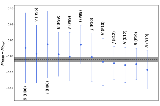
In this section we investigate the net effect on absolute magnitudes of SN Ia, either by adopting the TRGB or Cepheid distances. We approach this test separately for each of the 12 standardization methodology/bandpass combinations. With the purpose of separating from this test the systematics arising from drawing different nearby SNe from their parent population, for each methodology/bandpass combination we identify the same sample of nearby SNe having both Cepheid and TRGB distances. We obtain between five and ten SNe in common for each methodology/bandpass combination. We then calculate the absolute magnitude difference between the Cepheid and TRGB calibrations. Figure 1 presents the difference in absolute magnitude for each of the 12 methodology/bandpass combinations. In all cases the absolute magnitudes are systematically brighter when using the TRGB distances. On average the 12 combinations yield -=-0.0600.008 (). Since we use TRGB and Cepheid distance moduli anchored to the same R1 calibration, this comparison provides a direct estimate of the systematic difference between the TRGB and Cepheid distance moduli. This difference can be compared to the systematic uncertainties in the TRGB and Cepheid methods, of 0.033 mag (Freedman et al., 2019) and 0.030 mag (Riess et al., 2019), respectively (excluding the systematic uncertainty in the adopted LMC distance modulus). Adding in quadrature both terms we would expect a 0.044 mag difference in -, somewhat smaller than our derived value of -=-0.0600.008, thus suggesting that the systematic uncertainties calculated by Freedman et al. (2019) and/or Riess et al. (2019) might be somewhat underestimated.
3.2 Rung 3
Here we investigate the robustness of R3 of the CDL using the various surveys and techniques employed to deliver standardized SN luminosities for SNe Ia in the Hubble flow. As mentioned above, the scope of this work focuses on six prescriptions that make use of several distant samples of SNe Ia such as the Calán-Tololo, CfA, LOSS, and CSP.
The common approach in those analysis has been to establish the redshift-magnitude relationship, a.k.a. the Hubble diagram. Here the meaning of magnitude is a standardized peak brightness of a SN. Within the context of the Friedman-Lemaître cosmological model, the redshift-magnitude relationship takes the form,
| (1) |
where , is the luminosity distance of each SN, is the Hubble-Lemaître constant, and ZP is an empirically determined zero-point provided by the data. In the low redshift ( 0.1) regime, the redshift-magnitude relationship can be approximated by a simple kinematical model including an acceleration term,
| (2) |
where is the deceleration parameter. Within the aforementioned cosmological framework, ZP relates two physical quantities, and , in this simple way:
| (3) |
where is the standardized absolute peak magnitude of SNe Ia. Hence, the empirically derived ZP of the Hubble diagram interacts directly with the Hubble-Lemaître constant, and the peak absolute magnitude is the contact point between ZP and .
| Method | Published Zero Point (ZP′) | Zero Point (ZP)a |
|---|---|---|
| H96(B) | -3.3180.035 | -3.3840.035 b |
| H96(V) | -3.3290.031 | -3.3790.031 b |
| H96(I) | -3.0570.035 | -3.0870.035 b |
| P99(B) | 28.6710.043 | -3.6710.043 c |
| P99(V) | 28.6150.043 | -3.6150.043 c |
| P99(I) | 28.2360.037 | -3.2360.037 c |
| F10(J) | -18.440.01 | -2.7270.01 d |
| F10(H) | -18.380.02 | -2.6670.02 d |
| K12(J) | -18.5520.002 | -2.8390.002 d |
| K12(H) | -18.3900.003 | -2.6770.003 d |
| F19(B) | -19.1620.010 | -3.4490.010 d |
| R16(B) | -0.712730.00176 | -3.5640.009 e |
-
•
a .
-
•
b corrected for new Galactic Extinction Calibration, see section A.1.2.
-
•
c .
-
•
d .
-
•
e .
Each one of the six prescriptions selected for this work have different definitions for the zero points. Table 2 summarizes the original zero points published by their authors (ZP′), each of which is unique for each methodology and band-pass. By choice, we do not to modify them but, we convert all of them to the definition given in equation 1 in order to facilitate their comparison. Combining these zero points with the corresponding absolute magnitudes, we proceed to compute values using equation 3.
| Method | H0(B) | H0(V) | H0(I)/H0(i) | H0(J) | H0(H) | TRGB/CEPH |
|---|---|---|---|---|---|---|
| stat | stat | stat | stat | stat | ||
| H96 (no colour correction) | 72.9 2.7 | 71.3 2.2 | 69.8 2.6 | – | – | TRGB |
| H96 (with colour correction) | 66.6 2.5 | 66.6 2.1 | 67.1 2.5 | – | – | TRGB |
| P99 | 70.2 2.0 | 70.1 1.9 | 68.7 1.8 | – | – | TRGB |
| F10 | – | – | – | 66.5 1.6 | 69.4 2.1 | TRGB |
| K12 | – | – | – | 69.2 1.2 | 70.3 1.6 | TRGB |
| F19 (Tripp method) | 70.0 1.0 | – | – | – | – | TRGB |
| R19 | 70.4 1.2 | – | – | – | – | TRGB |
| H96 (no colour correction) | 77.0 2.6 | 76.3 2.1 | 72.5 2.7 | – | – | CEPH |
| H96 (with colour correction) | 72.4 2.5 | 72.8 2.0 | 70.6 2.6 | – | – | CEPH |
| P99 | 75.0 2.0 | 75.4 1.9 | 72.4 1.8 | – | – | CEPH |
| F10 | – | – | – | 69.1 1.3 | 74.4 1.6 | CEPH |
| K12 | – | – | – | 72.7 1.0 | 75.2 1.2 | CEPH |
| F19 (Tripp method) | 72.4 1.1 | – | – | – | – | CEPH |
| R19 | 73.8 1.2 | – | – | – | – | CEPH |
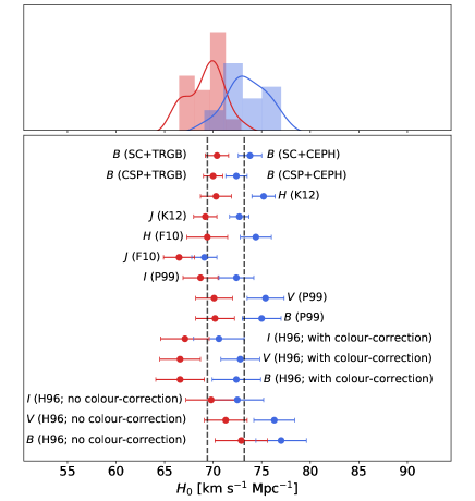
In Table 3 and Figure 2 we present the 30 values derived from the 12 methodology/bandpass combinations, using both the TRGB and the Cepheid calibrations, as described in Appendix A. Given the systematic differences found for R2 in section 3.1, we present the TRGB and Cepheid with different colors. As anticipated, there is a clear offset between both distributions. From the TRGB calibration we obtain a weighted average of 69.41.9 () . Looking in more detail to the distribution, we note that the most discrepant value is F10(J) with 66.51.6, which lies 1.8 from the mean. Interestingly, the recalibration by K12 gives a value of 69.21.2, and lies comfortably close to the mean value, which suggests that the F10(J) value may be subject to a significant systematic uncertainty. Although the H96 values derived with no colour corrections are formally consistent with the average, they tend to lie on the high side of the distribution, with a systematic decrease from the , , and bands. This trend disappears when using the colour-corrected values 444This improvement is expected due to the fact that the original H96 analysis did not apply host-galaxy reddening corrections to individual SNe but only the removal of suspicious SNe having near-maximum colour 0.2, that is, those most likely affected by host reddening. This simple colour cutoff leaves little room for significant extinction on the parent galaxies but may introduce a luminosity bias due to unaccounted differential host-galaxy extinction between the distant and the nearby samples. The application of a global colour correction between both samples is a statistical approach that helps to reduce such bias, as clearly shown in Figure 2.. The Cepheid calibration yields a weighted average of 73.22.1 () . As in the TRGB distribution, we note again that the most discrepant value is F10(J) with 69.11.3, which lies 3.2 from the mean, but the band recalibration by K12 provides a value of 72.71.0, solving this issue. We note again that the H96 methodology behaves better when using colour-corrected values.
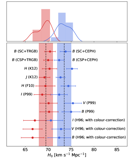
Based on the previous analysis, we show in Figure 3 our results but we eliminate the suspicious values, that is, the six H96 values derived with no color correction and the two F10(J) values. From this subset of 11 methodologies/bandpass we obtain similar averages but with smaller standard deviations, namely, 69.51.5 () for the TRGB calibration and 73.51.5 () for the Cepheid calibration. Adding in quadrature the systematic uncertainty in the TRGB method of 0.033 mag (Freedman et al., 2019) and in the Cepheid technique of 0.030 mag (Riess et al., 2019) (excluding the systematic uncertainty in the adopted LMC distance modulus), the systematic offset between the TRGB and Cepheid calibrations can be clearly seen, with a significance of 1.6 .
We can now go a step further and attempt to measure the error in the mean for each of the two distributions. However, given that several of the 11 methodologies/bandpass combinations considered above do not use entirely independent data, the resulting values are not fully independent from each other, thus implying that the error on the mean cannot be blindly computed from the 11 values. To get around this issue, we select the three most independent possible methodologies/bandpasses: P99(V), K12(J), and R19(B). The first two datasets are fully independent as they do not have any SN in common in the Hubble flow used to determine the ZP. The last two datasets are not fully independent, but only 11% of the Supercal sample employed by R19 overlap with the CSP sample used by K12. We reproduce such values in Table 4, and we present the weighted mean and the error in the mean. For the TRGB calibration we obtain =69.90.8, while for the Cepheid method we derive =73.50.7 . Adding in quadrature the systematic uncertainty in the TRGB method of 0.033 mag (Freedman et al., 2019) and in the Cepheid technique of 0.030 mag (Riess et al., 2019) (excluding the systematic uncertainty in the adopted LMC distance modulus), this exercise reveals a significant 2.0 systematic difference in the calibration of R2. However, if R1 and R2 are held fixed, the different formalisms developed for standardizing the SN peak magnitudes yield consistent results. This study demonstrates that SNe Ia have provided a remarkably robust calibration of R3 for over 25 years!
| Method | TRGB/CEPH | |
|---|---|---|
| P99(V) | 70.11.9 | TRGB |
| K12(J) | 69.21.2 | TRGB |
| R19(B) | 70.41.2 | TRGB |
| Weighted Mean | 69.90.8 | TRGB |
| P99(V) | 75.41.9 | CEPH |
| K12(J) | 72.71.0 | CEPH |
| R19(B) | 73.81.2 | CEPH |
| Weighted Mean | 73.50.7 | CEPH |
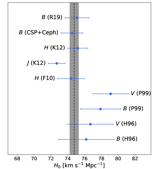
We turn now to the challenge of estimating the systematic error in based on SNe Ia, taking advantage of the large number of methodology/bandpass combinations presented in this study. To address this issue we compare values derived from the same subset of nearby objects. This approach allows us to isolate the systematics of these formulations from those introduced by the sample of nearby SNe that each methodology draws from the parent population of nearby SNe. We purposely exclude from this study the F10(J) value as well as those obtained using H96 and no colour correction for the reasons mentioned above. With such constraints we are able to carry out this test using nine SNe in common to nine methodology/bandpass combinations calibrated with Cepheid distances. The values calculated with these constraints are shown in Figure 4. The weighted mean =74.8 has an associated standard deviation of 2.0, which is mainly dominated by the statistical uncertainties of the small sample of nearby SNe (n=9). The value of 1.25 indicates that the statistical uncertainties are capable of accounting for most of the dispersion. An small extra uncertainty of 0.2 lowers to unity, which can be attributed to systematic uncertainties in these methods. An upper limit to the systematic uncertainties can be estimated from the standard deviation which amounts to 2.0 , although the majority of it can be attributed to the statistical uncertainties. We repeated the same analysis but using the TRGB distances. In this case the sample of nearby SNe drops to only n=5, the standard deviation is 2.3 and is identical to unity.
4 Conclusions
We assess the robustness of the two highest rungs of the Cosmic Distance Ladder (CDL) for Type Ia supernovae and the corresponding determination of the Hubble-Lemaître constant. In this analysis we hold fixed the first rung of the CDL (R1) as the distance modulus to the LMC, 18.480.02, determined to a 1% precision level using DEB stars (Pietrzyński et al., 2019). For the second rung (R2) we analyze the two currently most competitive methods, the TRGB and Cepheid luminosity calibration of Type Ia supernovae in nearby galaxies. Finally, for the third rung of the CDL (R3) we analyze various modern digital samples of SNe Ia in the smooth Hubble flow, such as the Calán-Tololo, CfA, CSP, Supercal datasets, and six prescriptions to standardize their optical and NIR peak luminosities. We apply each of these six prescriptions to one or more bandpasses, leading to a total of 15 determinations of from all possible combinations of bandpasses and methodologies when using the TRGB calibration, and 15 additional determinations for the Cepheid calibration. This metadata analysis allowed us to draw the following conclusions:
No matter which SN sample, bandpass or methodology is employed for standardizing the SN luminosities, in all cases the F19 TRGB calibration yields smaller values than the R19 Cepheid calibration, a direct consequence of the systematic difference in the distance moduli calibrated from the TRGB and Cepheid methods. From the TRGB calibration we obtain a mean value of =69.51.5 (), whereas from the Cepheid method we find =73.51.5 . Adding in quadrature the systematic uncertainty in the TRGB method of 0.033 mag (Freedman et al., 2019) and in the Cepheid technique of 0.030 mag (Riess et al., 2019) (excluding the systematic uncertainty in the adopted LMC distance modulus), the systematic offset between the TRGB and Cepheid calibrations can be clearly seen, with a significance of 1.6 (see Fig. 3).
Selecting the three most independent possible methodologies/bandpasses (the band by Phillips et al. (1999), the band by Kattner et al. (2012), and the band by Riess et al. (2019)), we obtain =69.90.8 and =73.50.7 from the TRGB and Cepheid calibrations, respectively. Adding in quadrature the systematic uncertainty in the TRGB method of 0.033 mag (Freedman et al., 2019) and in the Cepheid technique of 0.030 mag (Riess et al., 2019) (excluding the systematic uncertainty in the adopted LMC distance modulus), this subset reveals a significant 2.0 systematic difference in the calibration of R2.
If R1 and R2 are held fixed, the different formalisms developed for standardizing the SN peak magnitudes yield consistent results, with a standard deviation of 1.5 that is, SNe Ia are able to anchor R3 to a level of 2% precision. This internal agreement yielded by SNe Ia, either using the TRGB or Cepheid calibrations, is remarkable as it comprises light curves of increasingly quality, starting with the Calán-Tololo sample, the first digital survey carried out in the early 90s, various releases of the CfA project, and the most modern CSP dataset obtained over recent years with a uniform photometric system over a wide range of optical and NIR bandpasses. This study demonstrates that SNe Ia have provided a remarkably robust calibration of R3 for over 25 years.
Acknowledgments
We thank Chris Burns for his kind and detailed responses to our inquiries about his analysis of the CSP data. We are grateful to Adam Riess and Chuck Bennett for sending us valuable comments on a previous version of this paper, which were incorporated into our study. This research has made use of the NASA/IPAC Extragalactic Database (NED) which is operated by the Jet Propulsion Laboratory, California Institute of Technology, under contract with the National Aeronautics and Space Administration. MH acknowledges support from the Hagler Institute of Advanced Study at Texas A&M University. NBS has been supported by the NSF grant AST-1613455 and the Mitchell/Heep/Munnerlyn Chair in Observational Astronomy. Additional support has come from the George P. and Cynthia Woods Mitchell Institute for Fundamental Physics and Astronomy.
DATA AVAILABILITY
All data used in this paper are available on request to the corresponding author.
References
- Addison et al. (2018) Addison G. E., Watts D. J., Bennett C. L., Halpern M., Hinshaw G., Weiland J. L., 2018, ApJ, 853, 119
- Alam et al. (2017) Alam S., et al., 2017, MNRAS, 470, 2617
- Beaton et al. (2016) Beaton R. L., et al., 2016, ApJ, 832, 210
- Benedict et al. (2007) Benedict G. F., et al., 2007, AJ, 133, 1810
- Burns et al. (2011) Burns C. R., et al., 2011, AJ, 141, 19
- Burns et al. (2014) Burns C. R., et al., 2014, ApJ, 789, 32
- Burns et al. (2018) Burns C. R., et al., 2018, ApJ, 869, 56
- Burstein & Heiles (1982) Burstein D., Heiles C., 1982, AJ, 87, 1165
- Buta & Turner (1983) Buta R. J., Turner A., 1983, PASP, 95, 72
- Cartier et al. (2014) Cartier R., et al., 2014, ApJ, 789, 89
- Contreras et al. (2010) Contreras C., et al., 2010, AJ, 139, 519
- Contreras et al. (2018) Contreras C., et al., 2018, ApJ, 859, 24
- Faber & Jackson (1976) Faber S. M., Jackson R. E., 1976, ApJ, 204, 668
- Feldmeier et al. (2007) Feldmeier J. J., Jacoby G. H., Phillips M. M., 2007, ApJ, 657, 76
- Filippenko et al. (2001) Filippenko A. V., Li W. D., Treffers R. R., Modjaz M., 2001, The Lick Observatory Supernova Search with the Katzman Automatic Imaging Telescope. p. 121
- Folatelli et al. (2010) Folatelli G., et al., 2010, AJ, 139, 120
- Foley et al. (2018) Foley R. J., et al., 2018, MNRAS, 475, 193
- Freedman et al. (2001) Freedman W. L., et al., 2001, ApJ, 553, 47
- Freedman et al. (2019) Freedman W. L., et al., 2019, ApJ, 882, 34
- Friedman et al. (2015) Friedman A. S., et al., 2015, ApJS, 220, 9
- Gall et al. (2018) Gall C., et al., 2018, A&A, 611, A58
- Ganeshalingam et al. (2010) Ganeshalingam M., et al., 2010, ApJS, 190, 418
- Giovanelli et al. (1997) Giovanelli R., Haynes M. P., da Costa L. N., Freudling W., Salzer J. J., Wegner G., 1997, ApJ, 477, L1
- Hamuy et al. (1991) Hamuy M., Phillips M. M., Maza J., Wischnjewsky M., Uomoto A., Landolt A. U., Khatwani R., 1991, AJ, 102, 208
- Hamuy et al. (1993a) Hamuy M., Phillips M. M., Wells L. A., Maza J., 1993a, PASP, 105, 787
- Hamuy et al. (1993b) Hamuy M., et al., 1993b, AJ, 106, 2392
- Hamuy et al. (1995) Hamuy M., Phillips M. M., Maza J., Suntzeff N. B., Schommer R. A., Aviles R., 1995, AJ, 109, 1
- Hamuy et al. (1996a) Hamuy M., Phillips M. M., Suntzeff N. B., Schommer R. A., Maza J., Aviles R., 1996a, AJ, 112, 2398
- Hamuy et al. (1996b) Hamuy M., et al., 1996b, AJ, 112, 2408
- Hamuy et al. (2006) Hamuy M., et al., 2006, PASP, 118, 2
- Hicken et al. (2009) Hicken M., et al., 2009, ApJ, 700, 331
- Hicken et al. (2012) Hicken M., et al., 2012, ApJS, 200, 12
- Hinshaw et al. (2013) Hinshaw G., et al., 2013, ApJS, 208, 19
- Hubble (1929) Hubble E., 1929, Proceedings of the National Academy of Science, 15, 168
- Jang & Lee (2015) Jang I. S., Lee M. G., 2015, ApJ, 807, 133
- Jang & Lee (2017) Jang I. S., Lee M. G., 2017, ApJ, 836, 74
- Jha et al. (2006) Jha S., et al., 2006, AJ, 131, 527
- Kattner et al. (2012) Kattner S., et al., 2012, PASP, 124, 114
- Kelly et al. (2010) Kelly P. L., Hicken M., Burke D. L., Mand el K. S., Kirshner R. P., 2010, ApJ, 715, 743
- Kowal (1968) Kowal C. T., 1968, AJ, 73, 1021
- Krisciunas et al. (2003) Krisciunas K., et al., 2003, AJ, 125, 166
- Krisciunas et al. (2017) Krisciunas K., et al., 2017, AJ, 154, 211
- Landolt (1992) Landolt A. U., 1992, AJ, 104, 340
- Lee et al. (1993) Lee M. G., Freedman W. L., Madore B. F., 1993, ApJ, 417, 553
- Lemaître (1927) Lemaître G., 1927, Annales de la Société Scientifique de Bruxelles, 47, 49
- Li et al. (2000) Li W. D., et al., 2000, in Holt S. S., Zhang W. W., eds, American Institute of Physics Conference Series Vol. 522, American Institute of Physics Conference Series. pp 103–106 (arXiv:astro-ph/9912336), doi:10.1063/1.1291702
- Lira (1996) Lira P., 1996, Master’s thesis, -
- Lira et al. (1998) Lira P., et al., 1998, AJ, 115, 234
- Marion et al. (2016) Marion G. H., et al., 2016, ApJ, 820, 92
- Olivares E.F et al. (2010) Olivares E.F F., et al., 2010, ApJ, 715, 833
- Pan et al. (2015) Pan Y. C., et al., 2015, MNRAS, 452, 4307
- Phillips (1993) Phillips M. M., 1993, ApJ, 413, L105
- Phillips et al. (1999) Phillips M. M., Lira P., Suntzeff N. B., Schommer R. A., Hamuy M., Maza J., 1999, AJ, 118, 1766
- Pietrzyński et al. (2019) Pietrzyński G., et al., 2019, Nature, 567, 200
- Planck Collaboration et al. (2018) Planck Collaboration et al., 2018, arXiv e-prints, p. arXiv:1807.06205
- Pskovskii (1977) Pskovskii I. P., 1977, Soviet Ast., 21, 675
- Reid et al. (2019) Reid M. J., Pesce D. W., Riess A. G., 2019, ApJ, 886, L27
- Ribas et al. (2005) Ribas I., Jordi C., Vilardell F., Fitzpatrick E. L., Hilditch R. W., Guinan E. F., 2005, ApJ, 635, L37
- Richmond & Smith (2012) Richmond M. W., Smith H. A., 2012, Journal of the American Association of Variable Star Observers (JAAVSO), 40, 872
- Richmond et al. (1995) Richmond M. W., et al., 1995, AJ, 109, 2121
- Riess et al. (1995) Riess A. G., Press W. H., Kirshner R. P., 1995, ApJ, 438, L17
- Riess et al. (1996) Riess A. G., Press W. H., Kirshner R. P., 1996, ApJ, 473, 88
- Riess et al. (1999) Riess A. G., et al., 1999, AJ, 117, 707
- Riess et al. (2005) Riess A. G., et al., 2005, ApJ, 627, 579
- Riess et al. (2016) Riess A. G., et al., 2016, ApJ, 826, 56
- Riess et al. (2019) Riess A. G., Casertano S., Yuan W., Macri L. M., Scolnic D., 2019, ApJ, 876, 85
- Rodríguez et al. (2014) Rodríguez Ó., Clocchiatti A., Hamuy M., 2014, AJ, 148, 107
- Rust (1974) Rust B. W., 1974, PhD thesis, Oak Ridge National Lab., TN.
- Saha et al. (1994) Saha A., Labhardt L., Schwengeler H., Macchetto F. D., Panagia N., Sandage A., Tammann G. A., 1994, ApJ, 425, 14
- Saha et al. (1995) Saha A., Sandage A., Labhardt L., Schwengeler H., Tammann G. A., Panagia N., Macchetto F. D., 1995, ApJ, 438, 8
- Saha et al. (1996) Saha A., Sandage A., Labhardt L., Tammann G. A., Macchetto F. D., Panagia N., 1996, ApJ, 466, 55
- Saha et al. (1999) Saha A., Sandage A., Tammann G. A., Labhardt L., Macchetto F. D., Panagia N., 1999, ApJ, 522, 802
- Sandage (1970) Sandage A. R., 1970, Physics Today, 23, 34
- Sandage et al. (1996) Sandage A., Saha A., Tammann G. A., Labhardt L., Panagia N., Macchetto F. D., 1996, ApJ, 460, L15
- Schlafly & Finkbeiner (2011) Schlafly E. F., Finkbeiner D. P., 2011, ApJ, 737, 103
- Schlegel et al. (1998) Schlegel D. J., Finkbeiner D. P., Davis M., 1998, ApJ, 500, 525
- Scolnic et al. (2015) Scolnic D., et al., 2015, ApJ, 815, 117
- Stahl et al. (2019) Stahl B. E., et al., 2019, MNRAS, 490, 3882
- Stritzinger et al. (2002) Stritzinger M., et al., 2002, AJ, 124, 2100
- Stritzinger et al. (2010) Stritzinger M., et al., 2010, AJ, 140, 2036
- Stritzinger et al. (2011) Stritzinger M. D., et al., 2011, AJ, 142, 156
- Sullivan et al. (2010) Sullivan M., et al., 2010, MNRAS, 406, 782
- Suntzeff (2000) Suntzeff N. B., 2000, in Holt S. S., Zhang W. W., eds, American Institute of Physics Conference Series Vol. 522, American Institute of Physics Conference Series. pp 65–74 (arXiv:astro-ph/0001248), doi:10.1063/1.1291696
- Suntzeff et al. (1999) Suntzeff N. B., et al., 1999, AJ, 117, 1175
- Tonry et al. (1997) Tonry J. L., Blakeslee J. P., Ajhar E. A., Dressler A., 1997, ApJ, 475, 399
- Tripp (1998) Tripp R., 1998, A&A, 331, 815
- Vilardell et al. (2010) Vilardell F., Ribas I., Jordi C., Fitzpatrick E. L., Guinan E. F., 2010, A&A, 509, A70
- Wells et al. (1994) Wells L. A., et al., 1994, AJ, 108, 2233
- Wong et al. (2019) Wong K. C., et al., 2019, arXiv e-prints, p. arXiv:1907.04869
- de Jaeger et al. (2015) de Jaeger T., et al., 2015, ApJ, 815, 121
- de Jaeger et al. (2020) de Jaeger T., Stahl B. E., Zheng W., Filippenko A. V., Riess A. G., Galbany L., 2020, arXiv e-prints, p. arXiv:2006.03412
- van Leeuwen et al. (2007) van Leeuwen F., Feast M. W., Whitelock P. A., Laney C. D., 2007, MNRAS, 379, 723
Appendix A
This appendix describes six prescriptions that allow one to calculate standardized absolute peak magnitudes for SNe Ia. We apply these recipes to the set of nearby SNe that possess either Cepheid or TRGB distances from R19 and F19, respectively. In the first four cases we employ the published prescription for measuring, in the first place, the standardized apparent peak magnitudes, after which we subtract the corresponding distance modulus. In the last two cases we omit the first step since the standardized apparent magnitudes are available in the literature. In each case we proceed to compute the corresponding values of by combining the absolute magnitudes with the zero point of the Hubble diagram derived, in each case, from SNe Ia in the Hubble flow.
A.1 The H96 methodology
The Hamuy et al. (1996a) methodology was developed to analyze the sample of 29 distant SNe Ia obtained in the course of the Calán-Tololo project, which constituted the first sample of SNe in the Hubble flow observed with modern linear CCD detectors. Maximum light magnitudes in the bands and the decline rate parameter were measured for each SN (H96c). A Hubble diagram was obtained for each band, after correcting the peak magnitudes for the Galactic reddening provided by BH82, K-terms (H93b), and decline rate . Although the individual SNe were not corrected for host-galaxy reddening, three outlier objects were removed from the initial sample having the pseudo-colour 0.2, that is, those most likely affected by host reddening. This simple colour cutoff left little room for significant extinction on the parent galaxies. In fact, the weighted average pseudo-colour of the 26 remaining SNe, 0.0070.013 (), is quite normal for unextinxguished SNe Ia. All of the above led to Hubble diagrams with remarkably low dispersions of 0.17, 0.14, 0.13 mag, in , , , respectively, thus opening the path to high precision cosmology (H96). Cepheid distances measured with HST by Sandage, Saha, and collaborators to the host galaxies of SNe 1937C, 1972E, 1981B, 1990N (Saha et al., 1994; Saha et al., 1995, 1996; Sandage et al., 1996) allowed the calibration of the Calán-Tololo Hubble diagram and derive a value of 635 for the Hubble-Lemaître constant.
A.1.1 Absolute Magnitudes
We use now the H96 methodology to determine absolute magnitudes for the 18 nearby SNe Ia with TRGB distances published by F19, in the same manner as done for the distant SNe. A requisite to include such SNe in the re-analysis of the Calán-Tololo data is that each object must have available photometry in the Landolt standard photometric system (Landolt, 1992), which means that the reduced magnitudes include a photometric colour term (of course, this color term is not correct for SNe, and an S-correction (Stritzinger et al., 2002) is normally needed, but since we are applying the original H96 formula, no correction is needed for this purpose). Two of the nearby SNe, SN 2007on and SN 2007sr, do not fulfill this condition. For the remaining SNe we measure their peak magnitudes directly from the data, using a simple Legendre polynomial, as explained in section 3. Following H96, we exclude all SNe with 0.2, namely, SN 1989B and SN 1998bu, which reduced to 14 the number of SNe with TRGB distances.
Table 5 summarizes our measurements for such nearby SNe (14 in and , and 8 in the filter), including their TRGB distances, peak magnitudes, decline rate, from the NASA Extragalactic Database (NED), the source for the photometry, and the SN peak absolute magnitudes corrected for Galactic reddening and decline rate (to the fiducial value of =1.1). The uncertainty in an individual absolute magnitude is the result of adding in quadrature the uncertainties in peak magnitude, Galactic extinction, distance modulus, decline rate, the slope of the peak magnitude-decline rate relation, and an additional term amounting to 0.05 mag that we attribute to the fact that the SN magnitudes were not corrected for S-terms (Suntzeff, 2000; Stritzinger et al., 2002). Although the lack of S-correction constitutes a systematic uncertainty for an individual magnitude, they should tend to behave randomly for the ensemble of data points.
For each of the bands, we proceed to compute the weighted mean absolute magnitude corrected for (), the weighted standard deviation (), the standard error of the mean (), and the error of the weighted mean. Note that the standard deviations for the local SNe are 0.26 mag in , 0.22 in , and 0.20 in , that is, 0.07 mag greater, in all three bands, than the scatter yielded by the SNe in the Hubble flow which ranges between 0.17-0.13 mag. Possible explanations for the increase in the scatter could be due to unaccounted host-galaxy extinction corrections in the nearby sample or uncertainties in the host galaxies distances.
In view that the H96 method applied a simple colour cut to correct the SNe for host-galaxy extinction, it proves relevant to compare the colours of the nearby SNe with those in the Hubble flow. We analyze first the TRGB sample of 14 nearby SNe. For this dataset the weighted mean colour, after correcting for Galactic extinction (Schlafly & Finkbeiner, 2011), is 0.0370.019 (). For the distant sample the corresponding color is -0.0100.013. It is possible that this difference could be due to unaccounted differential host-galaxy extinction between the distant and the nearby samples. Hence, we decide to compute a mean absolute magnitudes by forcing the nearby sample to have the same bluer colour of the distant sample. This required decreasing the previous values by (0.037+0.010)/, where =4.16, =3.14, =1.82. Table 5 includes mean absolute magnitudes corrected for colour.
Now we apply the H96 technique to nearby SNe with Cepheid distances published by the SH0ES program. Again, to be consistent with H96 we restrict the sample of nearby SNe to those with 0.2 and magnitudes in the Landolt standard system. These two restrictions permit us to apply this method to 17 nearby SNe in and , and 9 SNe in the filter. Table 6 presents the relevant parameters of the SNe, the distance moduli published by R16 to which we added a global correction of -0.029 mag (=log 73.24/74.22) in order to place them in the R19 Cepheid scale, and the resulting mean absolute magnitude corrected for . This set of 17 nearby SNe with Cepheid distances has a mean colour, corrected for Galactic extinction (Schlafly & Finkbeiner, 2011), of 0.0220.018 (), that is, redder than the -0.0100.013 color of the distant sample. Table 6 includes mean absolute magnitudes computed by forcing the nearby sample to have the same color of the distant sample.
A.1.2 The Hubble-Lemaître constant
Having determined absolute magnitudes, it is straightforward to compute with the formula:
| (4) |
where, is the mean absolute magnitude of the nearby SNe corrected for decline rate and foreground extinction (given in Tables 5 and 6), and is the zero-point of the Hubble diagram.
The zero points of the Hubble diagrams derived by H96 were -3.318, -3.329, -3.057, respectively. These values need to be corrected owing to the fact that the Galactic extinction applied by H96 to the distant sample (Burstein & Heiles, 1982) differs from the new calibration (Schlafly & Finkbeiner, 2011) that we use for the nearby SNe. Given that the Burstein & Heiles (1982) calibration yielded a mean correction of 0.031 mag for the ensemble of 26 distant SNe, and the new calibration of Schlafly & Finkbeiner (2011) yields a somewhat greater correction of 0.047 mag, we have to decrease the zero points of the Hubble diagrams to -3.384, -3.379, -3.087 in , , and , respectively.
We analyze first the TRGB sample of nearby SNe. Given the discussion above about the color difference between the nearby and distant samples, we decide to calculate two sets of solutions: one ignoring the colour difference between both samples and one that forces both samples to have the same colour. Without taking into account colour differences we obtain (B)=72.9, (V)=71.3, and (V)=69.8. Correcting for colour differences between the nearby (redder) and distant (bluer) samples, the resulting values are lower than those derived without correcting for color difference and much more consistent among the three filters: 66.6, 66.6, and 67.1 for , , and , respectively. If there was significant differential reddening between the nearby and distant sample, we should observe a dependence of the value as a function of wavelength, which is not the case. Hence, it is encouraging that the colour correction yields values nearly independent on the band considered. The resulting values for are summarized in Table 3, with and without color correction.
Now we analyze the Cepheid sample of nearby SNe in the same manner as above for the TRGB sample. Without considering colour differences we derive (B)=77.0, (V)=76.3, and (V)=72.5. Forcing both datasets to match the same colour, we obtain values of 72.4, 72.8, and 70.6 for , , and , respectively, which are internally consistent within the statistical uncertainties. The resulting values for are summarized in Table 3. As can be seen in this table, the values derived using the H96 methodology are in excellent agreement with those derived from modern and larger datasets such as the CSP or Supercal. The Hubble flow from 1996 was sufficient to derive the modern value of the Hubble-Lemaître constant. We only had to wait until a better calibration of the distance to Cepheids and an improved reddening map were made.
| SN | Galaxy | Distance | Photometry | ||||||||
| Name | Modulus | 0.020 | Source | ||||||||
| SF11 | |||||||||||
| SN 1980N | N1316 | 31.46(0.04) | 12.49(0.02) | 12.44(0.02) | 12.71(0.10) | 1.28(0.04) | 0.020 | -19.194(0.116) | -19.210(0.100) | -18.890(0.130) | Hamuy et al. (1991) |
| SN 1981B | N4536 | 30.96(0.05) | 12.03(0.03) | 11.93(0.03) | – | 1.10(0.07) | 0.017 | -19.001(0.126) | -19.083(0.111) | – | Buta & Turner (1983) |
| SN 1981D | N1316 | 31.46(0.04) | 12.59(0.04) | 12.40(0.04) | – | 1.44(0.05) | 0.020 | -19.220(0.134) | -19.363(0.116) | – | Hamuy et al. (1991) |
| SN 1994D | N4526 | 31.00(0.07) | 11.89(0.02) | 11.90(0.02) | 12.06(0.05) | 1.31(0.08) | 0.021 | -19.362(0.142) | -19.314(0.126) | -19.099(0.121) | Richmond et al. (1995) |
| SN 1994ae | N3370 | 32.27(0.05) | 13.19(0.02) | 13.10(0.02) | 13.35(0.03) | 0.86(0.05) | 0.029 | -19.012(0.126) | -19.091(0.109) | -18.835(0.099) | Riess et al. (1999) |
| SN 1995al | N3021 | 32.22(0.05) | 13.38(0.02) | 13.24(0.02) | 13.52(0.05) | 0.83(0.05) | 0.013 | -18.682(0.128) | -18.830(0.111) | -18.568(0.109) | Riess et al. (1999) |
| SN 2001el | N1448 | 31.32(0.06) | 12.84(0.02) | 12.73(0.02) | 12.80(0.04) | 1.15(0.05) | 0.014 | -18.577(0.123) | -18.669(0.108) | -18.574(0.100) | Krisciunas et al. (2003) |
| SN 2002fk | N1309 | 32.50(0.07) | 13.30(0.03) | 13.37(0.03) | 13.57(0.03) | 1.02(0.04) | 0.038 | -19.295(0.128) | -19.193(0.115) | -18.953(0.102) | Cartier et al. (2014) |
| SN 2006dd | N1316 | 31.46(0.04) | 12.30(0.05) | 12.27(0.05) | 12.46(0.05) | 1.28(0.05) | 0.020 | -19.384(0.127) | -19.380(0.112) | -19.140(0.099) | Stritzinger et al. (2010) |
| SN 2007af | N5584 | 31.82(0.10) | 13.29(0.02) | 13.25(0.02) | – | 1.26(0.04) | 0.038 | -18.814(0.147) | -18.802(0.135) | – | Krisciunas et al. (2017) |
| SN 2011fe | M101 | 29.08(0.04) | 10.02(0.04) | 9.96(0.04) | 10.23(0.04) | 1.15(0.04) | 0.008 | -19.132(0.117) | -19.180(0.102) | -18.893(0.087) | Richmond & Smith (2012) |
| SN 2011iv | N1404 | 31.42(0.05) | 12.48(0.03) | 12.49(0.03) | – | 1.77(0.05) | 0.010 | -19.507(0.171) | -19.435(0.146) | – | Gall et al. (2018) |
| SN 2012cg | N4424 | 31.00(0.06) | 12.11(0.03) | 11.99(0.03) | – | 0.92(0.04) | 0.019 | -18.828(0.126) | -18.942(0.112) | – | Marion et al. (2016) |
| SN 2012fr | N1365 | 31.36(0.05) | 12.02(0.02) | 12.04(0.02) | – | 0.82(0.04) | 0.020 | -19.204(0.126) | -19.185(0.109) | – | Contreras et al. (2018) |
| Mean (no color correction) | -19.072 | -19.113 | -18.866 | ||||||||
| Mean (color correction) | -19.267 | -19.261 | -18.951 | ||||||||
| 0.269 | 0.225 | 0.209 | |||||||||
| / | 0.072 | 0.060 | 0.074 | ||||||||
| Error in Mean | 0.035 | 0.030 | 0.037 | ||||||||
| 14 | 14 | 8 |
| SN | Galaxy | Distance | Photometry | ||||||||
| Name | Modulus | 0.020 | Source | ||||||||
| SF11 | |||||||||||
| SN 1981B | N4536 | 30.877(053) | 12.03(0.03) | 11.93(0.03) | – | 1.10(0.07) | 0.017 | -18.918(0.127) | -19.000(0.112) | – | Buta & Turner (1983) |
| SN 1990N | N4639 | 31.503(071) | 12.76(0.03) | 12.70(0.02) | 12.94(0.02) | 1.07(0.05) | 0.012 | -18.769(0.130) | -18.819(0.115) | -18.568(0.101) | Lira et al. (1998) |
| SN 1994ae | N3370 | 32.043(049) | 13.19(0.02) | 13.10(0.02) | 13.35(0.03) | 0.86(0.05) | 0.029 | -18.785(0.125) | -18.864(0.109) | -18.608(0.099) | Riess et al. (1999) |
| SN 1995al | N3021 | 32.469(090) | 13.38(0.02) | 13.24(0.02) | 13.52(0.05) | 0.83(0.05) | 0.013 | -18.931(0.148) | -19.079(0.134) | -18.817(0.133) | Riess et al. (1999) |
| SN 1998aq | N3982 | 31.708(069) | 12.35(0.02) | 12.46(0.02) | 12.69(0.02) | 1.09(0.04) | 0.000 | -19.350(0.125) | -19.241(0.111) | -19.012(0.098) | Riess et al. (2005) |
| SN 2001el | N1448 | 31.282(045) | 12.84(0.02) | 12.73(0.02) | 12.80(0.04) | 1.15(0.05) | 0.014 | -18.539(0.116) | -18.631(0.101) | -18.536(0.091) | Krisciunas et al. (2003) |
| SN 2002fk | N1309 | 32.494(055) | 13.30(0.03) | 13.37(0.03) | 13.57(0.03) | 1.02(0.04) | 0.038 | -19.289(0.121) | -19.187(0.106) | -18.947(0.092) | Cartier et al. (2014) |
| SN 2003du | U9391 | 32.890(063) | 13.44(0.04) | 13.55(0.04) | 13.84(0.02) | 1.09(0.05) | 0.000 | -19.442(0.129) | -19.333(0.115) | -19.044(0.095) | Hicken et al. (2009) |
| SN 2005cf | N5917 | 32.234(102) | 13.63(0.02) | 13.56(0.02) | – | 1.03(0.04) | 0.077 | -18.869(0.146) | -18.866(0.135) | – | Hicken et al. (2009) |
| SN 2007af | N5584 | 31.757(046) | 13.29(0.02) | 13.25(0.02) | – | 1.26(0.04) | 0.038 | -18.751(0.117) | -18.739(0.102) | – | Krisciunas et al. (2017) |
| SN 2009ig | N1015 | 32.468(081) | 13.58(0.04) | 13.46(0.02) | – | 0.86(0.04) | 0.015 | -18.762(0.143) | -18.885(0.125) | – | Hicken et al. (2012) |
| SN 2011by | N3972 | 31.558(070) | 12.94(0.02) | 12.89(0.02) | 12.97(0.02) | 1.07(0.04) | 0.000 | -18.594(0.125) | -18.647(0.112) | -18.571(0.098) | Stahl et al. (2019) |
| SN 2011fe | M101 | 29.106(045) | 10.02(0.04) | 9.96(0.04) | 10.23(0.04) | 1.15(0.04) | 0.008 | -19.158(0.119) | -19.206(0.105) | -18.919(0.090) | Richmond & Smith (2012) |
| SN 2012cg | N4424 | 31.051(292) | 12.11(0.03) | 11.99(0.03) | – | 0.92(0.04) | 0.019 | -18.879(0.312) | -18.933(0.307) | – | Marion et al. (2016) |
| SN 2012fr | N1365 | 31.278(057) | 12.02(0.02) | 12.04(0.02) | – | 0.82(0.04) | 0.020 | -19.122(0.129) | -19.103(0.113) | – | Contreras et al. (2018) |
| SN 2012ht | N3447 | 31.879(043) | 13.11(0.02) | 13.10(0.02) | – | 1.29(0.04) | 0.012 | -18.968(0.118) | -18.951(0.102) | – | Burns et al. (2018) |
| SN 2015F | N2442 | 31.482(053) | 13.49(0.02) | 13.29(0.02) | – | 1.43(0.04) | 0.178 | -18.991(0.131) | -18.984(0.114) | – | Burns et al. (2018) |
| Mean (no color correction) | -18.952 | -18.967 | -18.784 | ||||||||
| Mean (color correction) | -19.085 | -19.067 | -18.842 | ||||||||
| 0.267 | 0.214 | 0.214 | |||||||||
| / | 0.065 | 0.052 | 0.071 | ||||||||
| Error in Mean | 0.032 | 0.028 | 0.033 | ||||||||
| 17 | 17 | 9 |
A.2 The P99 methodology
The Phillips et al. (1999) methodology improved the previous work by H96 by determining host-galaxy reddening to individual SNe through three novel independent methods: one based on the fact that the colour 30-90 days past maximum evolve in a similar manner for most SNe Ia use (a.k.a the “Lira Law”, Lira, 1996) a second one using a calibration of the colour with , and a third that calibrates the colour with . These techniques were tested using 62 SNe: 29 from the Calán-Tololo project, 20 objects from the CfA work (Riess et al., 1999), and 13 well-observed nearby SNe, whose peak magnitudes had been previously corrected for Galactic extinction using the calibration of Schlegel et al. (1998), and for K terms (Hamuy et al., 1993a).
When applied to a sample of 17 “low host-galaxy reddening” SNe with decline rates of 0.85 <<1.7, a well-behaved peak magnitude-decline rate relation emerged, which was modeled with a quadratic function of the form = a [ -1.1] + b [ -1.1]2 with dispersions of 0.11, 0.09, and 0.13 mag in , respectively, clearly lower than the ones obtained by H96 in the bands.
After applying these corrections due to host-galaxy reddening to the 40 SNe in the Hubble flow ( >0.01), P99 obtained Hubble diagrams in the bands, with dispersions of 0.14 mag. The resulting Hubble diagrams were combined with the six SN peak magnitudes calibrated with Cepheid distances (Saha et al., 1999; Suntzeff et al., 1999), which led to a value of =63.32.23.5 .
A.2.1 Absolute Magnitudes
Now we apply the P99 technique to nearby SNe with TRGB distances. To be consistent with P99 we restrict the sample of nearby SNe to those meeting the following two requirements: (1) having photometry in the Landolt standard photometric system, and (2) lying in the range 0.85 <<1.7. This restriction permits us to apply this method to 15 nearby SNe in and , and 10 SNe in the filter.
We follow the same procedure described in P99, that is, we measure peak magnitudes, decline rates, and host-galaxy reddening directly from the light curves (in the same manner described above in A.1.1), which are summarized in Table 7. The mean magnitudes for the ensemble of SNe (shown at the bottom of Table 7) are characterized by dispersions between 0.14-17 mag, that is, 0.04 mag greater than those yielded by the distant samples, possibly due to uncertainties in the TRGB distances.
Now we apply the P99 technique to nearby SNe with Cepheid distances, restricting the sample to those SNe with magnitudes in the Landolt standard system lying in the range 0.85 <<1.7. This restriction permits us to apply this method to 18 nearby SNe in and , and 10 SNe in the filter. Table 8 presents the relevant parameters of the SNe along with the distance moduli published by R16 to which we add a global correction of -0.029 mag (= 5 log 73.24/74.22) in order to place them in the R19 Cepheid scale.
A.2.2 The Hubble-Lemaître constant
For the P99 implementation the value of can be obtained with the formula:
| (5) |
where, is the mean absolute magnitude of the nearby SNe corrected for decline rate, foreground and host-galaxy extinction (given in Tables 7 and 8), and is the zero-point of the Hubble diagram.
The zero points of the Hubble diagrams derived by P99 were 28.671, 28.615, 28.236, respectively. We note that P99 used the Schlegel et al. (1998) corrections for Galactic reddening, whereas the values in Tables 7 and 8 are in the modern Schlafly & Finkbeiner (2011) calibration, which could be a potential source of systematic error for the derivation of . However, we checked that this difference has a negligible effect in our results (0.002 mag difference in for the full sample of 62 SN host galaxies).
Combining the SN peak magnitudes calibrated with TRGB distances with the zero points of the Hubble diagrams derived by P99, we obtain values of 70.2, 70.1, and 68.7 in , respectively, in good internal agreement given their statistical uncertainty of 2 (see Table 3).
Now we apply the P99 technique to nearby SNe with Cepheid distances. The resulting values for range between 72 and 75 (see Table 3). There is an excellent match with the values obtained using the H96 method, thus confirming that the 26 Calán-Tololo SNe were not significantly extinguished by host-galaxy dust compared to the nearby SNe calibrated with the Cepheid method.
| SN | Galaxy | Distance | Photometry | |||||||||
| Name | Modulus | 0.020 | Source | |||||||||
| SF11 | ||||||||||||
| SN 1980N | N1316 | 31.46(0.04) | 12.49(0.02) | 12.44(0.02) | 12.71(0.10) | 1.28(0.04) | 0.019 | 0.05(0.02) | -19.381(0.167) | -19.339(0.147) | -18.932(0.160) | Hamuy et al. (1991) |
| SN 1981D | N1316 | 31.46(0.04) | 12.59(0.04) | 12.40(0.04) | – | 1.44(0.05) | 0.019 | 0.20(0.06) | -19.980(0.332) | -19.907(0.283) | – | Hamuy et al. (1991) |
| SN 1981B | N4536 | 30.96(0.05) | 12.03(0.03) | 11.93(0.03) | – | 1.10(0.07) | 0.016 | 0.11(0.03) | -19.462(0.198) | -19.433(0.170) | – | Buta & Turner (1983) |
| SN 1989B | N3627 | 30.22(0.04) | 12.34(0.05) | 11.99(0.05) | 11.75(0.05) | 1.31(0.07) | 0.029 | 0.34(0.04) | -19.562(0.252) | -19.513(0.218) | -19.208(0.183) | Wells et al. (1994) |
| SN 1998bu | N3368 | 30.31(0.04) | 12.20(0.03) | 11.88(0.03) | 11.67(0.05) | 1.01(0.05) | 0.022 | 0.33(0.03) | -19.521(0.183) | -19.493(0.153) | -19.256(0.126) | Suntzeff et al. (1999) |
| SN 1994D | N4526 | 31.00(0.07) | 11.89(0.02) | 11.90(0.02) | 12.06(0.05) | 1.32(0.05) | 0.020 | 0.00(0.02) | -19.335(0.190) | -19.280(0.172) | -19.039(0.161) | Richmond et al. (1995) |
| SN 1994ae | N3370 | 32.27(0.05) | 13.19(0.02) | 13.10(0.02) | 13.35(0.03) | 0.86(0.05) | 0.027 | 0.12(0.03) | -19.479(0.208) | -19.445(0.182) | -19.059(0.156) | Riess et al. (1999) |
| SN 1995al | N3021 | 32.22(0.05) | 13.38(0.02) | 13.24(0.02) | 13.52(0.05) | 0.83(0.05) | 0.012 | 0.15(0.03) | -19.271(0.215) | -19.276(0.189) | -18.846(0.170) | Riess et al. (1999) |
| SN 2001el | N1448 | 31.32(0.06) | 12.84(0.02) | 12.73(0.02) | 12.80(0.04) | 1.15(0.05) | 0.013 | 0.17(0.03) | -19.289(0.188) | -19.206(0.159) | -18.879(0.131) | Krisciunas et al. (2003) |
| SN 2002fk | N1309 | 32.50(0.07) | 13.30(0.03) | 13.37(0.03) | 13.57(0.03) | 1.02(0.04) | 0.035 | 0.01(0.04) | -19.321(0.218) | -19.214(0.180) | -18.975(0.137) | Cartier et al. (2014) |
| SN 2006dd | N1316 | 31.46(0.04) | 12.30(0.05) | 12.27(0.05) | 12.46(0.05) | 1.28(0.05) | 0.019 | 0.07(0.03) | -19.655(0.202) | -19.573(0.175) | -19.219(0.147) | Stritzinger et al. (2010) |
| SN 2007af | N5584 | 31.82(0.10) | 13.29(0.02) | 13.25(0.02) | – | 1.26(0.04) | 0.035 | 0.09(0.05) | -19.164(0.268) | -19.058(0.223) | – | Krisciunas et al. (2017) |
| SN 2011fe | M101 | 29.08(0.04) | 10.02(0.04) | 9.96(0.04) | 10.23(0.04) | 1.15(0.04) | 0.008 | 0.09(0.05) | -19.511(0.245) | -19.465(0.195) | -19.051(0.137) | Richmond & Smith (2012) |
| SN 2012cg | N4424 | 31.00(0.06) | 12.11(0.03) | 11.99(0.03) | – | 0.92(0.04) | 0.018 | 0.20(0.05) | -19.648(0.255) | -19.567(0.208) | – | Marion et al. (2016) |
| SN 2012fr | N1365 | 31.36(0.05) | 12.02(0.02) | 12.04(0.02) | – | 0.82(0.04) | 0.018 | -0.01(0.11) | -19.102(0.491) | -19.106(0.384) | – | Contreras et al. (2018) |
| Mean | -19.439 | -19.385 | -19.050 | |||||||||
| 0.171 | 0.174 | 0.146 | ||||||||||
| / | 0.044 | 0.045 | 0.046 | |||||||||
| Error in Mean | 0.057 | 0.048 | 0.047 | |||||||||
| 15 | 15 | 10 |
| SN | Galaxy | Distance | Photometry | |||||||||
| Name | Modulus | 0.020 | Source | |||||||||
| SF11 | ||||||||||||
| SN 1981B | N4536 | 30.877(0.053) | 12.03(0.03) | 11.93(0.03) | – | 1.10(0.07) | 0.016 | 0.11(0.03) | -19.379(0.199) | -19.350(0.171) | – | Buta & Turner (1983) |
| SN 1990N | N4639 | 31.503(0.071) | 12.76(0.03) | 12.70(0.02) | 12.94(0.02) | 1.07(0.05) | 0.023 | 0.09(0.03) | -19.196(0.191) | -19.143(0.161) | -18.760(0.129) | Lira et al. (1998) |
| SN 1994ae | N3370 | 32.043(0.049) | 13.19(0.02) | 13.10(0.02) | 13.35(0.03) | 0.86(0.05) | 0.027 | 0.12(0.03) | -19.252(0.208) | -19.218(0.181) | -18.832(0.156) | Riess et al. (1999) |
| SN 1995al | N3021 | 32.469(0.090) | 13.38(0.02) | 13.24(0.02) | 13.52(0.05) | 0.83(0.05) | 0.012 | 0.15(0.03) | -19.520(0.227) | -19.525(0.204) | -19.095(0.186) | Riess et al. (1999) |
| SN 1998aq | N3982 | 31.708(0.069) | 12.35(0.02) | 12.46(0.02) | 12.69(0.02) | 1.09(0.04) | 0.012 | 0.02(0.06) | -19.485(0.284) | -19.343(0.224) | -19.073(0.154) | Riess et al. (2005) |
| SN 2001el | N1448 | 31.282(0.045) | 12.84(0.02) | 12.73(0.02) | 12.80(0.04) | 1.15(0.05) | 0.013 | 0.17(0.03) | -19.251(0.184) | -19.168(0.154) | -18.841(0.125) | Krisciunas et al. (2003) |
| SN 2002fk | N1309 | 32.494(0.055) | 13.30(0.03) | 13.37(0.03) | 13.57(0.03) | 1.02(0.04) | 0.035 | 0.01(0.04) | -19.315(0.214) | -19.208(0.174) | -18.969(0.130) | Cartier et al. (2014) |
| SN 2003du | U9391 | 32.890(0.063) | 13.44(0.04) | 13.55(0.04) | 13.84(0.02) | 1.09(0.05) | 0.009 | 0.01(0.05) | -19.522(0.253) | -19.394(0.204) | -19.081(0.145) | Hicken et al. (2009) |
| SN 2005cf | N5917 | 32.234(0.102) | 13.63(0.02) | 13.56(0.02) | – | 1.03(0.04) | 0.086 | 0.06(0.09) | -19.158(0.406) | -19.087(0.318) | – | Hicken et al. (2009) |
| SN 2007af | N5584 | 31.757(0.046) | 13.29(0.02) | 13.25(0.02) | – | 1.26(0.04) | 0.035 | 0.09(0.05) | -19.101(0.252) | -18.995(0.205) | – | Krisciunas et al. (2017) |
| SN 2009ig | N1015 | 32.468(0.081) | 13.58(0.04) | 13.46(0.02) | – | 0.86(0.04) | 0.029 | 0.10(0.12) | -19.210(0.529) | -19.225(0.410) | – | Hicken et al. (2012) |
| SN 2011by | N3972 | 31.558(0.070) | 12.94(0.02) | 12.89(0.02) | 12.97(0.02) | 1.07(0.04) | 0.013 | 0.13(0.04) | -19.198(0.214) | -19.105(0.176) | -18.841(0.132) | Stahl et al. (2019) |
| SN 2011fe | M101 | 29.106(0.045) | 10.02(0.04) | 9.96(0.04) | 10.23(0.04) | 1.15(0.04) | 0.008 | 0.09(0.05) | -19.537(0.246) | -19.491(0.196) | -19.077(0.138) | Richmond & Smith (2012) |
| SN 2012cg | N4424 | 31.051(0.292) | 12.11(0.03) | 11.99(0.03) | – | 0.92(0.04) | 0.018 | 0.19(0.05) | -19.661(0.383) | -19.589(0.354) | – | Marion et al. (2016) |
| SN 2012fr | N1365 | 31.278(0.057) | 12.02(0.02) | 12.04(0.02) | – | 0.82(0.04) | 0.018 | -0.01(0.11) | -19.020(0.492) | -19.024(0.385) | – | Contreras et al. (2018) |
| SN 2012ht | N3447 | 31.879(0.043) | 13.11(0.02) | 13.10(0.02) | – | 1.29(0.04) | 0.026 | 0.01(0.03) | -19.046(0.193) | -18.997(0.165) | – | Burns et al. (2018) |
| SN 2013dy | N7250 | 31.470(0.078) | 13.30(0.02) | 12.95(0.02) | 12.95(0.02) | 0.84(0.04) | 0.135 | 0.20(0.10) | -19.336(0.451) | -19.373(0.354) | -18.992(0.239) | Pan et al. (2015) |
| SN 2015F | N2442 | 31.482(0.053) | 13.49(0.02) | 13.29(0.02) | – | 1.43(0.04) | 0.180 | 0.09(0.05) | -19.308(0.291) | -19.195(0.251) | – | Burns et al. (2018) |
| Mean | -19.297 | -19.229 | -18.938 | |||||||||
| 0.166 | 0.168 | 0.129 | ||||||||||
| / | 0.039 | 0.040 | 0.041 | |||||||||
| Error in Mean | 0.058 | 0.049 | 0.046 | |||||||||
| 18 | 18 | 10 |
A.3 The F10 METHODOLOGY
The decade of the 90s meant a breakthrough for the measurement of the expansion rate of the Universe using SNe Ia, thanks to the gathering of digital CCD photometry of several dozens of SNe in the Hubble flow. However, the analysis of such data promptly revealed that the transformation of the instrumental magnitudes to the standard photometric system was rendered challenging owing to the non-stellar nature of the SN spectral energy distributions. Differences of several hundreds of a magnitude were noticed in the light curves of the same objects observed with different instruments (Suntzeff, 2000; Stritzinger et al., 2002). An additional difficulty in the standardization of SNe Ia as distance indicators arose from the effects of dust extinction in the SN parent galaxies which, despite the efforts to determine them from the observed SN colours, introduced significant uncertainties more strongly on the bluer wavelengths. These problems were addressed by the Carnegie Supernova Program (CSP) launched in 2004 (Hamuy et al., 2006) from Las Campanas Observatory (LCO) which, after nearly a decade of effort, led to the gathering of high-quality optical/NIR () lightcurves of 134 SNe Ia light curves in the Hubble flow with stable instrumental systems, namely, the Swope 1m and the du Pont 2.5m telescopes.
Contreras et al. (2010) published the first data release (DR1) of 34 SN light curves observed between 2004-2006. Since the observations were consistently obtained with the same instrumental bandpasses, the instrumental magnitudes were converted to the natural system through the application of a zero point and no colour term, thus avoiding the difficulty of transforming the data to the standard photometric system.
Following on the approach of P99, this high-quality dataset allowed F10 to derive an improved derivation of the “Lira law”, as well as better relationships between near-maximum reddening-free colours and , with a precision between 0.06-0.14 mag (see their table 3). Each of these ten calibrations allowed them to derive precise colour-excesses and study in depth the reddening law caused by host-galaxy dust.
The colour excesses were then used to re-examine the correlation of reddening-corrected absolute peak magnitudes versus decline rate, in the same manner as in P99, and re-assess the precision to which SNe Ia could be used as standardizable candles. As shown in their equation (7) the following two-parameter model was adopted:
| (6) |
where the three measured variables are , the peak apparent magnitude of the SN in a given band X corrected for K terms and Galactic reddening (Schlegel et al., 1998), , the colour excess due to host-galaxy dust obtained from bands Y and Z, the decline rate , and the distance modulus derived from the host-galaxy redshift and the cosmological parameters =0.72, =0.28, and =72 (see their equation 5). In this model there are three fitting parameters: the slope of the luminosity versus decline-rate, , the slope of the luminosity versus colour-excess, , and the peak absolute magnitude of the SNe Ia with =1.1 and zero colour-excess, . Their Table 5 shows results of the fits for ten (X,Y,Z) combinations, from the 23 “Best-observed” SN subsample, which are characterized by rms dispersions between 0.12-0.15 mag. These fits are restricted to the range 0.7 <<1.7 over which the colour excess calibrations are valid.
A.3.1 Absolute Magnitudes
Table 9 summarizes the input parameters for the six nearby SNe having TRGB distances and for which we are able to apply the F10 technique, that is, SNe with (1) NIR photometry available in the natural CSP system and (2) having decline rates within the range 0.7 <<1.7. Two of these six SNe were observed by the CSP (SN 2007af and SN 2012fr), two were observed with other instruments but were transformed to the Swope system via S-corrections (SN 2001el and SN 2006dd), one was observed with the FLWO/PAIRITEL instrument and converted from the 2MASS to the CSP system using the offsets determined by Contreras et al. (2010) (SN 2012cg), and one observed with the LCO du Pont WIRC instrument (SN 2002fk) which is virtually identical to the CSP photometric system. We measure peak magnitudes, decline rates, and colour excesses directly from the light curves, from which we compute standardized absolute peak magnitudes as follows,
| (7) |
where is the TRGB distance modulus. The resulting values are given in Table 9. The mean absolute magnitudes are shown at the bottom of Table 9 for the and bands (we omit the results for the remaining bands which only have two SNe calibrated with the TRGB method). The nearby SNe yield a dispersion in the standardized absolute magnitudes of 0.12 and 0.14 mag in and , respectively, in good agreement with the expected values yielded by the distant sample.
Now we apply the same technique for the nine SNe having Cepheid distances and and photometry. Four of these nine SNe were observed by the CSP (SN 2007af, SN 2012fr, SN 2012ht, and SN 2015F), one was observed with other instruments but was transformed to the Swope system via S-corrections (SN 2001el), three were observed with the FLWO/PAIRITEL instrument and converted from the 2MASS to the CSP system using the offsets determined by Contreras et al. (2010) (SN 2005cf, SN 2011by, and SN 2012cg), and one was observed with the LCO du Pont WIRC instrument which is virtually identical to the CSP photometric system (SN 2002fk). Table 10 presents the relevant parameters of the SNe along with the distance moduli published by R16 to which we add a global correction of -0.029 mag (= 5 log 73.24/74.22) in order to place them in the R19 Cepheid scale.
A.3.2 The Hubble-Lemaître constant
Armed with the SN standardized peak magnitudes we turn now to the determination of the value of by means of the following expression:
| (8) |
where is the mean absolute magnitude in a given band X corrected for foreground extinction, decline rate, and colour excess, derived from the nearby SNe, while is the standardized peak absolute magnitude derived by F10 from the distant SNe Ia, namely -18.440.01 and -18.380.02 in and , respectively. The resulting values using the TRGB distance moduli are (J)=66.51.6 and (H)=69.42.1 (see Table 3). Adopting the Cepheid distances, we obtain (J)=69.11.3 and (H)=74.41.6 , respectively (see Table 3). We note that there is a 2.6 difference between both values. As shown in the next section the updated NIR CSP calibration by K12 significantly alleviates this tension between the and bands.
| SN | Galaxy | Distance | corr | corr | Photometry | |||||
| Name | Modulus | 0.020 | Source | |||||||
| SF11 | ||||||||||
| SN 2001el | N1448 | 31.32(0.06) | 12.73(0.02) | 12.90(0.04) | 13.08(0.04) | 1.15(0.05) | 0.014 | -18.517(0.084) | -18.335(0.084) | Krisciunas et al. (2003) |
| SN 2002fk | N1309 | 32.50(0.07) | 13.37(0.03) | 13.76(0.02) | 13.98(0.02) | 1.02(0.04) | 0.038 | -18.755(0.080) | -18.537(0.079) | Cartier et al. (2014) |
| SN 2006dd | N1316 | 31.46(0.04) | 12.31(0.02) | 12.73(0.05) | 12.84(0.05) | 1.08(0.04) | 0.020 | -18.761(0.072) | -18.665(0.071) | Stritzinger et al. (2010) |
| SN 2007af | N5584 | 31.82(0.10) | 13.18(0.03) | 13.45(0.02) | 13.62(0.02) | 1.23(0.04) | 0.038 | -18.507(0.108) | -18.295(0.108) | Krisciunas et al. (2017) |
| SN 2012cg | N4424 | 31.00(0.06) | 11.99(0.03) | 12.34(0.05) | 12.52(0.04) | 0.92(0.04) | 0.019 | -18.619(0.088) | -18.491(0.087) | Marion et al. (2016) |
| SN 2012fr | N1365 | 31.36(0.05) | 11.99(0.02) | 12.73(0.02) | 12.96(0.02) | 0.83(0.04) | 0.020 | -18.490(0.067) | -18.304(0.077) | Contreras et al. (2018) |
| Mean | -18.614 | -18.459 | ||||||||
| 0.129 | 0.156 | |||||||||
| / | 0.053 | 0.064 | ||||||||
| Error in Mean | 0.033 | 0.034 | ||||||||
| 6 | 6 |
| SN | Galaxy | Distance | corr | corr | Photometry | |||||
| Name | Modulus | 0.020 | Source | |||||||
| SF11 | ||||||||||
| SN 2001el | N1448 | 31.282(0.045) | 12.73(0.02) | 12.90(0.04) | 13.08(0.04) | 1.15(0.05) | 0.014 | -18.479(0.074) | -18.297(0.074) | Krisciunas et al. (2003) |
| SN 2002fk | N1309 | 32.494(0.055) | 13.37(0.03) | 13.76(0.02) | 13.98(0.02) | 1.02(0.04) | 0.038 | -18.749(0.068) | -18.531(0.066) | Cartier et al. (2014) |
| SN 2005cf | N5917 | 32.234(0.102) | 13.56(0.02) | 13.82(0.05) | 13.95(0.05) | 1.01(0.04) | 0.086 | -18.469(0.119) | -18.345(0.119) | Hicken et al. (2009) |
| SN 2007af | N5584 | 31.757(0.046) | 13.18(0.03) | 13.45(0.02) | 13.62(0.02) | 1.23(0.04) | 0.038 | -18.444(0.062) | -18.232(0.062) | Krisciunas et al. (2017) |
| SN 2011by | N3972 | 31.558(0.070) | 12.89(0.03) | 13.19(0.02) | 13.48(0.05) | 1.13(0.04) | 0.013 | -18.437(0.081) | -18.121(0.091) | Friedman et al. (2015); Stahl et al. (2019) |
| SN 2012cg | N4424 | 31.051(0.292) | 11.99(0.03) | 12.34(0.05) | 12.52(0.04) | 0.92(0.04) | 0.019 | -18.670(0.299) | -18.542(0.299) | Marion et al. (2016) |
| SN 2012fr | N1365 | 31.278(0.057) | 11.99(0.02) | 12.73(0.02) | 12.96(0.02) | 0.83(0.04) | 0.020 | -18.408(0.072) | -18.222(0.082) | Contreras et al. (2018) |
| SN 2012ht | N3447 | 31.879(0.043) | 13.06(0.02) | 13.45(0.02) | 13.62(0.02) | 1.25(0.04) | 0.026 | -18.553(0.059) | -18.334(0.060) | Burns et al. (2018) |
| SN 2015F | N2442 | 31.482(0.053) | 13.26(0.02) | 13.12(0.05) | 13.42(0.10) | 1.23(0.04) | 0.180 | -18.637(0.082) | -18.222(0.120) | Burns et al. (2018) |
| Mean | -18.529 | -18.309 | ||||||||
| 0.119 | 0.127 | |||||||||
| / | 0.040 | 0.042 | ||||||||
| Error in Mean | 0.026 | 0.027 | ||||||||
| 9 | 9 |
A.4 THE K12 METHODOLOGY
Kattner et al. (2012) reanalized the standardization of SNe Ia in the NIR, in a similar manner as F10, but limiting the CSP sample to the 27 best-observed SNe, namely, those having pre-maximum coverage in optical bands and, particularly the sub-sample of 13 objects also having having pre-maximum NIR observations. The latter condition is particularly relevant since, as shown by F10, the extrapolation of peak magnitudes using NIR template light curves could introduce significant errors.
The correlation between peak absolute luminosity and decline rate was investigated using the same equation first proposed by P99,
| (9) |
where the measured quantities are , the peak apparent magnitude of the SN in a given band X (X=Y,J,H) corrected for K terms and Galactic reddening (Schlegel et al., 1998), , the decline rate measured from the -band, and , the colour excess due to host-galaxy reddening derived from the near-maximum reddening-free - colour derived by F10. As in F10, the left-hand term of this equation is the distance modulus derived from the host-galaxy redshift and the cosmological parameters =0.72, =0.28, and =72. In this model is the total-to-selective absorption coefficient for band X, a fixed parameter of =1.18, =0.89, =0.57, for an adopted =3.1 dust extinction law. In this model there are two fitting parameters: the slope of the luminosity versus decline-rate relation, , and the peak absolute magnitude of the SNe Ia with =1.1 and zero colour-excess, .
Their Table 5 shows results of the fits for the three NIR bands (,,) and five different sub-samples of SNe. Here we use sub-sample 3, which uses SNe Ia with first observations starting within five days after NIR peak brightness and excludes the highly reddened and fast-declining events. The correlations are characterized by rms dispersions between 0.09-0.12 mag. These fits are restricted to the range 0.7 <<1.7 over which the colour excess calibration is valid.
A.4.1 Absolute Magnitudes
We measure peak magnitudes, decline rates and colour excesses for the six nearby SNe having TRGB distances and for which we are able to apply the K12 technique, that is, SNe with (1) NIR photometry available in the natural CSP system and (2) having decline rates within the range 0.7 <<1.7. We compute standardized absolute peak magnitudes as follows,
| (10) |
where is the TRGB distance modulus. Table 11 summarizes the input parameters and their standardized absolute peak magnitudes for all six SNe. The mean value is shown at the bottom of Table 11 for the and different bands (we omit the -band as there are only two nearby SNe with TRGB distance). The nearby SNe yield dispersions in the corrected absolute magnitudes of 0.08 and 0.11 mag, similar to those obtained by the distant sample.
Now we apply the K12 technique to the sample of nine nearby SNe with Cepheid distances and NIR photometry in the CSP natural system, and decline rates within the range 0.7 <<1.7. Table 12 presents the relevant parameters of the SNe along with the distance moduli published by R16 to which we add a global correction of -0.029 mag (= 5 log 73.24/74.22) in order to place them in the R19 Cepheid scale, and their corresponding standardized absolute peak magnitudes.
A.4.2 The Hubble-Lemaître constant
As in F10, the value of the Hubble-Lemaître constant can be calculated using the following expression:
| (11) |
where is the mean standardized absolute peak magnitude in a given band X corrected for foreground extinction, decline rate, and colour excess, derived from the nearby SNe, while is the standardized peak absolute magnitude derived by K12 from the distant SNe Ia, namely -18.5520.002 and -18.3900.003 in and , respectively.
As can be seen in Table 3, the values for obtained for and bands are 69.21.2 and 70.31.6, respectively. Adopting the Cepheid distances, the resulting values for from the and bands are 72.71.0 and 75.21.2 , respectively. As anticipated in the previous section, the K12 recalibration of the -band SN Ia luminosity clearly alleviates the tension between the and bands calibration derived from F10.
| SN | Galaxy | Distance | corr | corr | Photometry | ||||||
| Name | Modulus | 0.020 | Source | ||||||||
| SF11 | |||||||||||
| SN 2001el | N1448 | 31.32(0.06) | 12.84(0.02) | 12.73(0.02) | 12.90(0.04) | 13.08(0.04) | 1.15(0.05) | 0.014 | -18.550(0.124) | -18.326(0.097) | Krisciunas et al. (2003) |
| SN 2002fk | N1309 | 32.50(0.07) | 13.30(0.03) | 13.37(0.03) | 13.76(0.02) | 13.98(0.02) | 1.02(0.04) | 0.038 | -18.673(0.127) | -18.473(0.099) | Cartier et al. (2014) |
| SN 2006dd | N1316 | 31.46(0.04) | 12.30(0.05) | 12.31(0.02) | 12.73(0.05) | 12.84(0.05) | 1.08(0.04) | 0.020 | -18.733(0.126) | -18.621(0.095) | Stritzinger et al. (2010) |
| SN 2007af | N5584 | 31.82(0.10) | 13.28(0.03) | 13.18(0.03) | 13.45(0.02) | 13.62(0.02) | 1.23(0.04) | 0.038 | -18.514(0.147) | -18.299(0.123) | Krisciunas et al. (2017) |
| SN 2012cg | N4424 | 31.00(0.06) | 12.11(0.03) | 11.99(0.03) | 12.34(0.05) | 12.52(0.04) | 0.92(0.04) | 0.019 | -18.733(0.133) | -18.518(0.101) | Marion et al. (2016) |
| SN 2012fr | N1365 | 31.36(0.05) | 12.03(0.02) | 11.99(0.02) | 12.73(0.02) | 12.96(0.02) | 0.83(0.04) | 0.020 | -18.606(0.120) | -18.371(0.090) | Contreras et al. (2018) |
| Mean | -18.638 | -18.442 | |||||||||
| 0.090 | 0.123 | ||||||||||
| / | 0.037 | 0.050 | |||||||||
| Error in Mean | 0.053 | 0.041 | |||||||||
| 6 | 6 |
| SN | Galaxy | Distance | corr | corr | Photometry | ||||||
| Name | Modulus | 0.020 | Source | ||||||||
| SF11 | |||||||||||
| SN 2001el | N1448 | 31.282(0.045) | 12.84(0.02) | 12.73(0.02) | 12.90(0.04) | 13.08(0.04) | 1.15(0.05) | 0.014 | -18.512(0.118) | -18.288(0.089) | Krisciunas et al. (2003) |
| SN 2002fk | N1309 | 32.494(0.055) | 13.30(0.03) | 13.37(0.03) | 13.76(0.02) | 13.98(0.02) | 1.02(0.04) | 0.038 | -18.667(0.120) | -18.467(0.090) | Cartier et al. (2014) |
| SN 2005cf | N5917 | 32.234(0.102) | 13.62(0.02) | 13.56(0.02) | 13.82(0.05) | 13.95(0.05) | 1.01(0.04) | 0.086 | -18.460(0.152) | -18.309(0.131) | Hicken et al. (2009) |
| SN 2007af | N5584 | 31.757(0.046) | 13.28(0.03) | 13.18(0.03) | 13.45(0.02) | 13.62(0.02) | 1.23(0.04) | 0.038 | -18.451(0.117) | -18.236(0.085) | Krisciunas et al. (2017) |
| SN 2011by | N3972 | 31.558(0.070) | 12.94(0.03) | 12.89(0.03) | 13.19(0.02) | 13.48(0.05) | 1.13(0.04) | 0.013 | -18.439(0.127) | -18.125(0.109) | Friedman et al. (2015); Stahl et al. (2019) |
| SN 2012cg | N4424 | 31.051(0.292) | 12.11(0.03) | 11.99(0.03) | 12.34(0.05) | 12.52(0.04) | 0.92(0.04) | 0.019 | -18.784(0.315) | -18.569(0.303) | Marion et al. (2016) |
| SN 2012fr | N1365 | 31.278(0.057) | 12.03(0.02) | 11.99(0.02) | 12.73(0.02) | 12.96(0.02) | 0.83(0.04) | 0.020 | -18.524(0.124) | -18.289(0.094) | Contreras et al. (2018) |
| SN 2012ht | N1365 | 31.879(0.043) | 13.09(0.02) | 13.06(0.02) | 13.45(0.02) | 13.62(0.02) | 1.25(0.04) | 0.020 | -18.516(0.113) | -18.323(0.082) | Burns et al. (2018) |
| SN 2015F | N2442 | 31.482(0.053) | 13.47(0.02) | 13.26(0.02) | 13.12(0.05) | 13.42(0.10) | 1.23(0.04) | 0.180 | -18.606(0.125) | -18.225(0.131) | Burns et al. (2018) |
| Mean | -18.530 | -18.297 | |||||||||
| 0.086 | 0.101 | ||||||||||
| / | 0.029 | 0.034 | |||||||||
| Error in Mean | 0.043 | 0.034 | |||||||||
| 9 | 9 |
A.5 THE F19 METHODOLOGY
Freedman et al. (2019) recently revisited the determination of from 99 CSP-I distant SNe using the light curve analysis developed by Burns et al. (2018, B18), in which the SN magnitudes are modeled using the light curve fitter SNooPy (Burns et al., 2011, 2014), which delivers for each SN its peak magnitudes corrected for K-terms and Galactic reddening, and which is the colour-stretch parameter (equivalent to the decline rate ). As described by B18, the standardization of the SN luminosities is performed using two approaches, the “Reddening” and the “Tripp” models . The former has the form,
| (12) |
Similarly to F10, this model computes peak magnitude corrections for decline rate (the linear and quadratic terms), and for host galaxy reddening using the colour excess derived from optical and NIR colours of each SN, but incorporates an additional correction due to the SN host galaxy stellar mass, , obtained from the -band magnitude of the host galaxy. In this equation is the SN observed peak magnitude in band and is the distance modulus computed from the SN host galaxy redshift given a set of cosmological parameters =72 , =0.27, and =0.73 (see Eq. (9) of B18). In this model there are five fitting parameters: the two polynomial coefficients that describe the luminosity versus stretch dependence, and , the slope of the luminosity versus colour-excess, , the slope of the luminosity versus host galaxy mass, , and (the peak absolute magnitude of a SN with =1, =0, =10). As shown by B18 the “Reddening” approach applied to the CSP SNe yields standardized absolute magnitudes with characteristic dispersions () between 0.08-0.12 mag, with the exception of the band where the scatter is 0.16 mag.
The second approach used by F19 is the “Tripp” model which has the form,
| (13) |
The main difference between the “Tripp” and the “Reddening” models is in the way the host galaxy reddening is addressed. Here the colour excess is replaced by , that is, the colour of the SN at peak. In other words, the reddening correction in the “Tripp” approach does not require to know the intrinsic colour of the SN, but neglects the fact that the intrinsic colour varies with decline rate. Thus, since the colour is affected both by the intrinsic and dust extinction effects, the inferred value of the parameter cannot be directly interpreted as a dust extinction law. As shown by B18 the “Tripp” approach applied to the CSP SNe yields standardized absolute magnitudes with characteristic dispersions () between 0.11-0.13 mag with a slight decrease toward longer wavelengths, except for the band where the scatter is significantly higher 0.22 mag.
A.5.1 Absolute Magnitudes
F19 presented in column 6 of Table 3 standardized apparent peak magnitudes in the -band for 27 nearby SNe, using the “Tripp” model. We employ such data in order to calculate absolute peak magnitudes using the 18 nearby SNe which have TRGB distances, from which we derive a mean value of =-19.2230.029, which compares well with the -19.2250.029 published by F19. Then we repeat the same procedure but this time using the 19 nearby SNe with Cepheid distances, which yield =-19.1500.033, after adding a correction of -0.029 mag (= 5 log 73.24/74.22) in order to place this value in the R19 Cepheid scale.
A.5.2 The Hubble-Lemaître constant
Freedman et al. (2019) applied the two approaches described by B18 to a subset of 99 CSP distant SNe with light curves and meeting the requirements <0.5 and >0.5, and presented in Table 5 individual values for the filters, using both the “Reddening” and the “Tripp” models. Here we attempt to reproduce their results but we face various problems, namely, (1) F19 published standardized apparent peak magnitudes for the nearby SNe only for the single case of the -band and the “Tripp” model (see their Table 3), (2) F19 did not publish the zero points of the distant Hubble diagram for any of the bands. Hence, we are only able to calculate the value of for that single case and presuming that F19 used the same zero point published by B18, namely =-19.162 (see their Table 1). For this purpose we employ the formula,
| (14) |
where we compute using the same data published in Table 3 of F19 ( and and adopt from B18. Our result, presented in Table 3, =70.01.0, is 0.5% higher than the published value by F19, namely 69.71.4 , thus implying that F19 did not exactly use the zero point derived by B18. Given the relevance of this topic, it is important that F19 make available all the necessary ingredients required to reproduce their results.
We repeat the same exercise but this time adopting the Cepheid distance moduli listed in Table 3 of F19 (with the only caveat that we add a correction of -0.029 mag in order to place such values in the R19 Cepheid scale), from which we obtain =72.41.1 (see Table 3). This value can be compared to the corresponding value obtained by B18 using the same “Tripp” model, duly modified to the R19 scale, namely, =73.72.1 . The question that arises is, what causes this 1.3 difference? Although it may not seem statistically significant, it proves concerning considering that both used the same method for standardizing the CSP peak magnitudes, so that the difference likely originates in the the parameter, whose error (usually less than 0.01 mag) has an impact of less than 0.3 in (see equation 14).
A.6 THE R19 METHODOLOGY
R16 made a determination of the Hubble-Lemaître constant from a sample of 19 nearby SNe with Cepheid distances (the R16 Cepheid scale), combined with a sample of 217 distant SNe Ia observed with optical filters in the course of the CSP and CfA surveys. Their light curves were re-calibrated using the “Supercal” method developed by Scolnic et al. (2015) with the purpose to place different SN samples on a single, consistent photometric system. The resulting light curves were analyzed with the SALT2 light curve fitter model which delivers SN peak magnitudes standardized using a colour and a stretch parameter similar to .
Adopting this formalism, R16 obtained a -band Hubble diagram with a zero point of =0.712730.00176. When combined with the Cepheid distances to 19 nearby SNe obtained by the SH0ES program, R16 derived a value of =73.241.74 , anchored to NGC 4258, the Milky Way and the LMC. More recently, R19 presented an improved determination of from Hubble Space Telescope (HST) observations of Cepheids in the LMC. Using only the LMC DEBs to calibrate the Cepheid luminosities, R19 derived a 1.34% greater value than R16, namely, =74.221.82 .
A.6.1 Absolute Magnitudes
R16 presented in Table 5 standardized apparent peak magnitudes in the -band (column 3) for the 19 SNe with Cepheid distances (column 5). We employ such data in order to calculate absolute peak magnitudes, from which we derive a mean value of =-19.2510.036 in the R16 Cepheid scale. Unfortunately, R19 did not publish the individual Cepheid distances re-calibrated to the LMC distance alone. Despite this difficulty, we manage to add a correction of -0.029 mag (= 5 log 73.24/74.22) to the R16 distance moduli in order to place them in the R19 scale, from which we derive a mean absolute magnitude =-19.2220.036. Now we repeat the same procedure but this time using the subset of ten nearby SNe with TRGB distances (F19), from which we obtain =-19.3260.038, which is identical to that obtained by F19.
A.6.2 The Hubble-Lemaître constant
As mentioned above, R19 obtained =74.221.82 , when using solely the LMC DEBs to calibrate the Cepheid luminosities. Here we attempt to reproduce their result using their equation 9,
| (15) |
where is the mean standardized band peak magnitude -19.2220.036 in the R19 Cepheid scale and is the zero point of the band Hubble diagram, 0.712730.00176. Our result, presented in Table 3, =73.81.2 is 0.5% lower than the published value by Riess et al. (2019), most likely due to the fact that we do not have access to the individual R19 Cepheid distances. Applying this formula to the mean magnitude -19.3260.038 obtained from the ten TRGB distances, we obtain =70.41.2 .