The Value of Context:
Human versus Black Box Evaluators
Abstract
Machine learning algorithms are now capable of performing evaluations previously conducted by human experts (e.g., medical diagnoses). How should we conceptualize the difference between evaluation by humans and by algorithms, and when should an individual prefer one over the other? We propose a framework to examine one key distinction between the two forms of evaluation: Machine learning algorithms are standardized, fixing a common set of covariates by which to assess all individuals, while human evaluators customize which covariates are acquired to each individual. Our framework defines and analyzes the advantage of this customization—the value of context—in environments with high-dimensional data. We show that unless the agent has precise knowledge about the joint distribution of covariates, the benefit of additional covariates generally outweighs the value of context.
1 Introduction
“A statistical formula may be highly successful in predicting whether or not a person will go to a movie in the next week. But someone who knows that this person is laid up with a broken leg will beat the formula. No formula can take into account the infinite range of such exceptional events.” — Atul Gawande, Complications: A Surgeon’s Notes on an Imperfect Science
Predictions about people are increasingly automated using black-box algorithms. How should individuals compare evaluation by algorithms (e.g., medical diagnosis by a machine learning algorithm) with more traditional evaluation by human experts (e.g., medical diagnosis by a doctor)?
One important distinction is that black-box algorithms are standardized, fixing a common set of inputs by which to assess all individuals. Unless the inputs to the black box are exhaustive, additional information can (in some cases) substantially modify the interpretation of those inputs that have been acquired. For example, the context that a patient is currently fasting may change the interpretations of “dizziness” and “electrolyte imbalance,” and the context that a job applicant is an environmental activist may change how a prior history of arrest is perceived. If these auxiliary characteristics are not specified as inputs in the algorithm, the individual cannot supply them.
In contrast, individuals can often explain their unusual circumstances or characteristics to a human evaluator through conversation. Thus, even if the human evaluator considers fewer inputs than a black box algorithm does, these inputs may be better adapted to the individual being evaluated. The perception that humans are better able to take into account an individual’s unique situation is a significant factor in patient resistance to AI in healthcare (Longoni et al., 2019). Our objective is to understand when, and to what extent, this difference between human and machine evaluation matters.
Our contribution in this paper is twofold. First, we propose a theoretical framework that formalizes this distinction between human and black box evaluation. Second, we explain assumptions under which it will turn out that the the agent should prefer one form of evaluation over the other. We see our paper as a complement to a growing empirical literature that compares human versus black box evaluation. Here our goal is to conceptualize the difference between human and black box evaluators, and to clarify properties of the informational environment that are important for choosing between the two.
In our model, an agent is described by a binary covariate vector and a real-valued type (e.g., the severity of the agent’s medical condition). The type can be written as a function of the covariates, which we henceforth call the type function. Covariates are separated into standard covariates (e.g., medical history, lab tests, imaging scans) and nonstandard covariates (e.g., religious information, genetic data, wearable device data, and financial data).
We suppose that the agent may know how the standard covariates are correlated with the type, but cannot distinguish between the predictive roles of the nonstandard covariates. Formally, the agent has a belief over the type function, and we impose two assumptions on the agent’s prior. The first is a symmetry assumption that says that the agent’s prior over these functions is unchanged by permuting the labels and values of the nonstandard covariates. If we interpret the covariates as signals about the agent’s type, then uncertainty about the type function corresponds to uncertainty about the signal structure (à la model uncertainty, e.g., Acemoglu et al. (2015) and Morris and Yildiz (2019)). The second assumption fixes the unpredictability of the agent’s type to be constant in the total number of covariates. We impose this because in many applications, machine learning algorithms have millions of inputs, and yet cannot predict the outcome perfectly. Thus our “many covariates” limit does not represent a situation in which the total of amount of information grows large, but rather one in which the type function can be arbitrarily complex. We view these two assumptions as useful conceptual benchmarks, but subsequently show that neither are essential for our main results (see Section 5 for details).
The agent’s payoff is determined by his true type and an evaluation, which may be made either by a human evaluator or a black-box evaluator. In either case the evaluation is a conditional expectation of the agent’s type given the agent’s standard covariates and some fraction of the agent’s nonstandard covariates. But the sets of nonstandard covariates that are observed by the black box evaluator and the human evaluator differ in two ways.
First, the black box evaluator observes a larger fraction of the nonstandard covariates than the human evaluator does (since humans cannot process as much information as black box algorithms can). Second, the nonstandard covariates observed by the black box evaluator are a pre-specified set of algorithmic inputs, which are fixed across individuals. For example, a designer of a medical algorithm may specify a set of inputs including (among others) blood type, BMI, and smoking status. The black box algorithm learns a mapping from those inputs into the diagnosis. We view the human evaluator as instead uncovering nonstandard covariates during a conversation, where the specific path of questioning may vary across agents. Thus the human evaluator may end up learning about one individual’s sleep schedule but another individual’s financial situation.
Rather than modeling these conversations directly, we consider an upper bound on the agent’s payoff under human evaluation, where the covariates that the human observes are the ones that maximize the agent’s payoffs (subject to the human’s capacity constraint). We say that the agent prefers the black box if the agent’s expected payoffs are higher under black box evaluation even compared to these best-case conversations with the human.
This comparison essentially reduces to the question of whether the agent prefers an evaluator who observes a larger fraction of (non-targeted) nonstandard covariates about the agent, or an evaluator who observes a smaller but targeted fraction of nonstandard covariates.111This question is spiritually related to Akbarpour et al. (2024)’s comparison of the network diffusion value of a small number of targeted seeds versus a larger number of randomly selected seeds. Like them, we will find that a larger number of (non-targeted) inputs is superior, but the mechanisms behind these results are very different; in particular, network structure does not play a role in our results. Towards this comparison, we first introduce a benchmark, which is the expected payoff that the agent would receive if interacting with an evaluator who observes no nonstandard covariates. We define the value of context to be the improvement in the agent’s payoffs under best-case human evaluation, relative to this benchmark. The value of context thus quantifies the extent to which the agent’s payoffs can possibly be improved when the evaluator observes nonstandard covariates suited to that agent.
Our first main result says that under our assumptions on the agent’s prior, the expected value of context vanishes to zero as the number of covariates grows large. Thus even though there may be realizations of the type function given which the value of context is large, in expectation it is not. The contrapositive of this result is that if the expected value of context is high in some application, it must be that our assumptions on the prior do not hold, i.e., the agent has some ex-ante knowledge about the predictive roles of the nonstandard covariates.
We prove this result by studying the sensitivity of the evaluator’s expectation to the set of covariates that are revealed. Intuitively, a large value of context requires that the evaluator’s beliefs move sharply after observing certain nonstandard covariates. We show that the largest feasible change in the evaluator’s beliefs can be written as the maximum over a set of random variables, each corresponding to the movement in the evaluator’s beliefs for a given choice of covariates to reveal. The proof proceeds by first reducing this problem to studying the maximum of a growing sequence of (appropriately constructed) i.i.d. variables, and then applying a result from Chernozhukov et al. (2013) to show that this expected maximum concentrates on its expectation as the number of covariates grows large. We conclude by bounding this expectation and demonstrating that it vanishes.
We next use this result to compare the agent’s expected payoff under human and black box evaluation, when the total number of covariates is sufficiently large. We show that when the agent prefers a more accurate evaluation—formally, when the agent’s payoff is convex in the evaluation—the agent should (eventually) prefer an algorithmic evaluator with access to more covariates over a human evaluator to whom the agent can provide context. And when the agent’s payoff is concave in the evaluation, the conclusion is (eventually) reversed. We view these conclusions as relevant not only in the many-covariates limit: We quantify the number of covariates that is needed for our result to hold, and show that it can be quite small. For example, if the agent’s utility function satisfies mild regularity conditions, the Human evaluator observes 10% of covariates, and the Black Box evaluator observes 90%, of covariates, then our result holds as long as there are at least 14 covariates.
We subsequently strengthen our main results in two ways: First, we show that not only does the expected value of context vanish for each agent, but in fact the expected maximum value of context across agents also vanishes. Thus, the expected value of context is eventually small for everyone in the population. Second, we show that our main results extend when the agent and evaluator interact in a disclosure game, where the agent chooses which nonstandard covariates to reveal, and the evaluator makes inferences about the agent based on which covariates are revealed (given the agent’s equilibrium reporting strategy).
We conclude by examining the role of our assumptions about the agent’s prior, and the extent to which our results depend on them. First, we study two variations of our main model, in which the symmetry assumption is relaxed: In the first, we suppose that there is a “low-dimensional” set of covariates that relevant for predicting the agent’s type; in the second, we suppose that the agent knows ex-ante the predictive role of certain nonstandard covariates. In both of these settings, our main results extend partially but can also fail: For example, if the set of relevant covariates is sufficiently small that they can be fully disclosed to the evaluator, then the expected value of context typically will not vanish. Next we show that our results extend also in a model in which the predictability of the agent’s type is higher in environments with a larger number of covariates (thus relaxing our second asumption on the prior). Finally we provide an abstract learning condition under which our results extend: It is enough for the informativeness of each individual set of covariates to vanish as the total number of covariates grows large. Together with our main results, these extensions clarify different categories of informational assumptions under which the expected value of context does or does not turn out to be high.
Our model is not meant to be a complete description of the differences between human and black box evaluation. For example, we do not consider human or algorithmic bias (Kleinberg et al., 2017; Gillis et al., 2021), explainability (Yang et al., 2024), preferences for empathetic evaluators, or the possibility that the human evaluator has access to information that is not available to the algorithm (e.g., for privacy protection reasons as in Agarwal et al. (2023)). We also suppose that both evaluators form correct conditional expectations, thus abstracting away from the possibility of algorithmic overfitting and of bounded human rationality (e.g., as considered in Spiegler (2020) and Haghtalab et al. (2021)).222The problem of overfitting, while practically important, is a function of how the algorithm is trained. We are interested here in intrinsic differences between the qualitative nature of human and black box evaluation, which are difficult to resolve by training the algorithm differently. We leave extensions of our model that include these other interesting differences to future work.
1.1 Related Literature
Our paper is situated at the intersection of the literatures on learning (Section 1.1.1) and strategic information disclosure (Section 1.1.2), where our analysis is primarily differentiated from the previous frameworks by our assumption that the agent has model uncertainty (see Section 1.1.1). Our paper is also inspired by a recent empirical literature that compares human and AI evaluation, which we review in Section 1.1.3.
1.1.1 (Asymptotic) Learning
A large literature studies asymptotic learning and agreement across Bayesian agents (Blackwell and Dubins, 1962). Our main result (Theorem 3.1) can be viewed as bounding (in expectation) the differences in beliefs across Bayesian agents who are given different information. As in Vives (1992), Golub and Jackson (2012), Liang and Mu (2019), Harel et al. (2020), and Frick et al. (2023) among others, we quantify the rate of convergence in beliefs. The learning rates that we look at are, however, of a different nature from those studied previously. One important distinction is that these previous papers consider asymptotics as the total amount of information accumulates, while our analysis considers asymptotics with respect to a sequence of information structures that we show are increasingly less informative. A second important difference is that the classic learning models suppose that the agent updates to a signal with a known signal structure, while our agent has uncertainty over the signal structure (as in Acemoglu et al. (2015) and Morris and Yildiz (2019)). Our results characterize the informativeness of this signal in expectation, where the agent’s model uncertainty takes a particular (and new) form motivated by the applications we have in mind.
Finally, our paper is related to Di Tillio et al. (2021), which compares the informativeness of an unbiased signal to the informativeness of a selected signal whose realization is the maximum realization across i.i.d. unbiased signals. Again the key difference is our assumption of model uncertainty—that is, in Di Tillio et al. (2021), the signal structures that are being compared are deterministic and known, while in ours they are random and compared in expectation. In particular, our agent’s prior belief over signal structures can have support on signal processes which are not i.i.d. (for example, it may be that the meaning of one signal is dependent on the meaning of another).
1.1.2 Strategic Information Disclosure
Several literatures study persuasion via strategic information disclosure. Our model—in which the sender has private information about his type vector, and selectively chooses which elements to disclose to a naive receiver—is closest to models of disclosure of hard information (Dye, 1985; Grossman and Hart, 1980), in particular Milgrom (1981).333A similar model of information is considered in Glazer and Rubinstein (2004) and Antic and Chakraborty (2023). The key difference (which follows from our assumption of model uncertainty) is that our sender has uncertainty about how his reports are interpreted. Additionally, our focus is not on examining which incentive-compatible reporting strategy is optimal,444Indeed, in our main model we do not require choice of an incentive-compatible reporting strategy, since the receiver updates to the sender’s disclosure as if it were exogenous information. This is primarily for convenience—we show in Section 4.2 that our results extend in a disclosure game. but instead on asymptotic limits of belief manipulability as the number of components in the type vector grows large. This latter focus is special to our motivating applications.
Our model also has important differences from the other main strands of the persuasion literature. Unlike models of cheap talk (Crawford and Sobel, 1982), our agent chooses between messages whose meanings are fixed exogenously (through the realization of the joint distribution relating covariates to the type) rather than in an equilibrium. Unlike the literature on Bayesian persuasion (Kamenica and Gentzkow (2011)), our sender chooses which signal realization to share ex-post from a finite set of signal realizations, rather than committing to a flexibly chosen information structure ex-ante.555Thus, for example, Bayes plausibility is not satisfied in our setting—the sender’s expectation of the receiver’s expectation of the state (following disclosure) is generally not the prior expectation of the state. Indeed, our model gives the sender substantial power to influence the receiver’s beliefs relative to this previous literature. It is perhaps surprising, then, that despite the lack of constraints imposed on the sender, we find that the sender is extremely limited in his influence. In our model, this emerges because the sender has a limited choice from a set of information structures, whose informativeness (we show) is vanishing in the total number of covariates.666The covariates in our model play a similar role to attributes, although the literature on attributes has focused on choice of which attributes to learn about (e.g., Klabjan et al. (2014) and Liang et al. (2022)), rather than which attributes to disclose for the purpose of persuasion. An exception is Bardhi (2023), who studies a principal-agent problem in which a principal selectively samples attributes to influence an agent decision.
1.1.3 Human vs AI Evaluation
Recent empirical papers compare the accuracy of human evaluation with AI evaluation, finding that machine learning algorithms outperform experts in problems including medical diagnosis (Rajpurkar et al., 2017; Jung et al., 2017; Agarwal et al., 2023), prediction of pretrial misconduct (Kleinberg et al., 2017; Angelova et al., 2022), and prediction of worker productivity (Chalfin et al., 2016). Nonetheless, many individuals continue to distrust algorithmic predictions (Jussupow and Heinzl, 2020; Bastani et al., 2022; Lai et al., 2023). These findings motivate our goal of understanding whether individuals should prefer human evaluators, and when instead the replacement of human evaluation with algorithmic evaluation is welfare-improving for users, as suggested in Obermeyer and Emanuel (2016) among others.
In principle, human decision-making guided by algorithmic predictions should be superior to either human or algorithmic prediction alone. In practice the evidence is more mixed, with the provision of algorithmic recommendations sometimes leading human decision-makers to less accurate predictions (Hoffman et al., 2017; Angelova et al., 2022; Agarwal et al., 2023).777Other papers instead consider algorithmic prediction tools that take human evaluation as an input, with greater success towards improving accuracy (e.g., Raghu et al. (2019)). The question of how to aggregate human and machine evaluations is thus important but subtle, and depends on (among other things) whether human decision-makers understand the correlation between their information and that of the algorithm (McLaughlin and Spiess, 2022; Gillis et al., 2021; Agarwal et al., 2023). We abstract away from these complexities, focusing instead on (one aspect of) the more basic question of why human oversight is even necessary to begin with. We provide a tractable way of formalizing the advantage of human evaluation, and quantify the size of this advantage.
2 Model
2.1 Setup
Agents are each described by a binary covariate vector and a type (where ), which are structurally related by the function
We refer to henceforth as the type function. The distribution over covariate vectors is uniform in the population.888All of our results extend for arbitrary finite-valued covariates.
We refer to the covariates indexed to as standard covariates and the covariates indexed to as nonstandard covariates.
Example 1 (Job Interview).
Standard covariates describing a job applicant may include their work history, education level, college GPA, and the coding languages they know. Nonstandard covariates may include their social media activity (e.g., number of followers, posts, likes), wearable device data (e.g., sleep patterns, physical activity level), and hobbies (e.g., whether they are active readers, whether they enjoy extreme sports).
Example 2 (Medical Prediction).
Standard covariates describing a patient may include symptoms, prior diagnoses, family medical history, lab tests and imaging results. Nonstandard covariates may include the patient’s religious practices, genetic data, wearable device data, and financial data.999See Acosta et al. (2022) for further examples of nonstandard patient covariates that may be predictive, but which are not currently used by clinicians for medical evaluations.
An evaluation of the agent, , is described in the following section. The agent has a Lipschitz continuous utility function , which maps the evaluation and the agent’s true type into a payoff.
Example 3 (Higher Evaluations are Better).
The agent’s payoff is
for some increasing . This corresponds, for example, to an agent receiving a desired outcome (e.g., a loan or a promotion) with probability increasing in the evaluation.
Example 4 (More Accurate Evaluations are Better).
The agent’s payoff is
This corresponds to harms that are decreasing in the accuracy of the evaluation, e.g., medical prediction problems where more accurate evaluations are desired.
2.2 Evaluation of the agent
There are two evaluators: a black box evaluator, henceforth Black Box (it), and a human evaluator, henceforth Human (she). Both form evaluations as an expectation of the agent’s type given observed covariates, so we will introduce notation for these conditional expectations. For any covariate vector and subset of nonstandard covariates , let
| (2.1) |
be the set of all covariate vectors that agree with on the covariates with indices in . Further define
| (2.2) |
to be the conditional expectation of the agent’s type given their standard covariates and their nonstandard covariates with indices in . We use
to denote the agent’s payoff given this evaluation.
Both the human and black box evaluation take the form (2.2), but the observed sets of nonstandard covariates are different across the evaluators. Black Box observes the nonstandard covariates in the set where .101010One can instead assume that these nonstandard covariates are selected uniformly at random. This will not affect the results of this paper. Importantly, this set is held fixed across agents. So an individual with covariate vector receives the evaluation and payoff when evaluated by the Black Box.111111It is not important for our results that is common across individuals; what we require is that any randomness in is independent of the agent’s covariates and type. For example, if the set were drawn uniformly at random for each agent, our results would hold.
Human differs from Black Box in two ways. First, Human has a capacity of nonstandard covariates per agent, where (i.e., Human cannot process as many inputs as Black Box). Second, Human does not pre-specify which nonstandard covariates to observe, but rather learns these through conversation, and thus potentially observes different nonstandard covariates for each agent. For example, a doctor (evaluator) may pose different questions to different patients (agents) depending on their answers to previous questions. Or a job candidate (agent) might choose to disclose to an interviewer (evaluator) certain nonstandard covariates that are favorable to him.
Rather than modeling the complex process of a conversation, we study the quantity
| (2.3) |
which is the agent’s payoff when the posterior expectation about his type is based on those or fewer covariates that are best for him.
We can interpret this quantity as an upper bound for the agent’s payoffs under certain assumptions. First, if the evaluator selects which covariates to observe, then (2.3) is an upper bound on the agent’s possible payoffs across all possible evaluator selection rules. Second, if covariates are disclosed by the agent, but the evaluator updates to the disclosed covariates as if they had been chosen exogenously, then again (2.3) represents an upper bound on the agent’s possible payoffs.121212Jin et al. (2021) and Farina et al. (2023) report that the beliefs of experimental subjects falls somewhere in between this naive benchmark and equilibrium beliefs, since subjects do not completely account for the strategic nature of disclosure.
If however the covariates are disclosed by the agent in a disclosure game, and the evaluator accounts for the strategic nature of this disclosure, then whether (2.3) represents an upper bound will depend on what we assume that the agent knows at the time of disclosure.131313This is roughly because the agent can potentially “sneak in” information about the other covariates via the covariates that are revealed. We show in Section 4.2 that if the agent knows his entire covariate vector, then (2.3) need not upper bound every agent’s payoffs. Nevertheless, we present a different quantity that does upper bound the maximum payoff that any agent can obtain in this disclosure game, and show that our main results extend when we replace (2.3) with this quantity. To streamline the exposition we focus on the prior two interpretations (in which the human evaluator either selects the covariates herself or updates to the agent’s disclosures naively), and discuss disclosure games in Section 4.2.
2.3 Value of context
A key input towards understanding the comparison between Human and Black Box is quantifying the extent to which individualized context improves the agent’s payoffs.
Definition 2.1 (Value of Context).
The value of context for an agent with covariate vector and type is
i.e., the best possible improvement in the agent’s utility when the evaluator additionally observes up to covariates for the agent.
In general, the value of context depends on the type function as well as on the agent’s own covariate vector .141414The value of context given a specific function is spiritually related to the communication complexity of (Kushilevitz and Nisan, 1996).
Example 5 (High Value of Context).
Let , i.e., the agent’s payoff is the evaluation. Suppose is a standard covariate (observed no matter what), while are nonstandard covariates. The type is related to these covariates via the type function
For an agent who can reveal (up to) one covariate and whose covariate vector is , the value of context is , since revealing moves the expectation of his type from 0 to . This example corresponds to settings in which some nonstandard covariate substantially moderates the interpretation of a standard covariate. For such type functions , it is important for the evaluator to observe the right nonstandard covariates, and so the value of context can be large.
Example 6 (Low Value of Context).
Suppose the type function in the previous example is instead (leaving all other details of the example unchanged). Then the value of context is 0 for every agent. In this example, nonstandard covariates are irrelevant for predicting the type, so there is no value to the evaluator discovering the “right” covariates.
In what follows, we give the agent uncertainty about and characterize the agent’s expected value of context and expected payoffs, integrating over the agent’s belief about .151515If we interpret the covariates in our model as signals about the type, then the function relating covariates to type corresponds to the signal structure.
We do this for two reasons. First, in many applications it is not realistic to suppose that the agent knows . For example, a patient who anticipates that a diagnosis will be based on an image scan of his kidney may recognize that there are properties of the image that are indicative of whether he has the condition or not, but likely does not know what the relevant properties are, or how they determine the diagnosis.161616In the case of a job interview, the function may reflect particular subjective preferences of the firm, which are initially unknown to the agent.
Second, the case with uncertainty about turns out to yield a more elegant analysis than the one in which is known. That is, although the value of context for specific functions depends on details of that function and on the agent’s own covariate vector, there is a large class of prior beliefs (described in the following section) for which it is possible to draw strong detail-free conclusions about the expected value of context.
2.4 Model Uncertainty
We impose two assumptions on the agent’s prior belief about . Together, these assumptions deliver a setting in which many different structural relationships between the covariates and the type are possible (including both ones where the value of context is high and low), but ex-ante those relationships are not known.
The first assumption says that while the agent may know how standard covariates impact the type, he has no ex-ante knowledge about the roles of the nonstandard covariates.
Assumption 1 (Exchangeability).
For every realization of the standard covariates , the sequence
| (2.4) |
is finitely exchangeable.
The set ranges over all covariate vectors that share the standard covariate values . Assumption 1 says that the joint distribution of these types is ex-ante invariant to permutations of the labels and values of the nonstandard covariates. An agent whose prior satisfies Assumption 1 is thus agnostic about how the nonstandard covariates impact the type.
While our assumption of no prior knowledge about the role of nonstandard covariates is strong, it is consistent with our interpretation of the nonstandard covariates as those covariates for which there is little historical data about correlations. For example, if it were known that a higher GPA positively correlates with on-the-job performance, but not how a large number of social media followers predicts performance, then we would think of GPA as a standard covariate and the number of social media followers as a nonstandard covariate.
Assumption 1 does not restrict how the agent’s prior varies with , the number of covariates. In a model in which were drawn i.i.d. from a type-dependent distribution , the total quantity of information about would increase in the number of covariates, and the evaluator’s uncertainty about would vanish as grew large. This does not seem descriptive of real applications: credit scoring algorithms and healthcare algorithms use millions of covariates, but there remains substantial residual uncertainty about the agent’s type. We take the opposite extreme in which the predictability of the agent’s type is a primitive of the setting, which is held constant for all . In our model, is not a measure of the total quantity of information, but instead moderates the richness of the informational environment and the potential complexity of the mapping . Loosely speaking, as grows large, the agent has a more extensive set of words to describe a fixed unknown .171717As grows large, the smallest possible informational size of each covariate (in the sense of McLean and Postlewaite (2002)) vanishes. But we do not require each covariate to be equally informationally relevant in the realized function. So, for example, can be in the support of the agent’s beliefs for arbitrarily large (see Example 7).
Assumption 2 (Constant Unpredictability of ).
Fix any realization of the standard covariates , and let be defined as in (2.4) for each . Then for every pair , the sequence and the truncated sequence are identically distributed.
The statement of Assumption 2 formally depends on the ordering of types within the vector , since this determines which types appear in the truncated sequence . But if we further impose Assumption 1 (and we will always impose these assumptions jointly), then the ordering of types is irrelevant: That is, when Assumption 2 holds for one such ordering, it will hold for all orderings.
It is important to note that in our model, Assumptions 1 and 2 are placed ex-ante on the agent’s prior, and not ex-post on the realized function . For example, the function , which says that the only covariate that matters is , is strongly asymmetric ( is differentiated from the other covariates) and also features a single “large” covariate (the realization of completely determines ). Our assumptions do not rule out the possibility of this function. Rather, they require that if this function is considered possible, then certain other functions are as well.181818Assumption 1 requires that for every permutation , the function satisfying is also in the support of the agent’s beliefs.
Simple examples of priors satisfying these two assumptions are given below.
Example 7.
Example 8.
Priors that violate these assumptions include the following.
Example 9 (Only One Covariate is Relevant).
The type is equal to the value of the nonstandard covariate , where the index is drawn uniformly at random from . Then Assumption 1 fails.191919Suppose , and both covariates are nonstandard. Then under the agent’s prior, where while , and while . So the agent knows with certainty that but , in violation of Assumption 1. This example is consistent with exchangeability in the labels of the nonstandard covariates, but not with exchangeability in their realizations.
Example 10 (Higher Values are Better).
The value of is (independently) drawn from a uniform distribution on if , and (independently) drawn from a uniform distribution on if . Then Assumption 1 fails.
2.5 Expected Value of Context
We now define the expected value of context from the point of view of an agent who knows his covariate vector but does not know the function (and hence also does not know his type ). As we show in Section 4.1, the assumption that the agent knows is immaterial for the results.
Definition 2.2 (Expected Value of Context).
For every and covariate vector , the expected value of context is
This quantity tells us the extent to which context improves the agent’s payoffs in expectation.
We similarly compare evaluators based on the expected payoff that the agent receives.
Definition 2.3.
Consider any agent with covariate vector . If
| (2.5) |
then say that the agent prefers the black box evaluator. And if
| (2.6) |
then say that the agent prefers the human evaluator.
These definitions correspond to a thought experiment in which (for example) a patient has a choice between being seen by a doctor or assessed by an algorithm. If the patient chooses the algorithm, his standard covariates and arbitrarily chosen nonstandard covariates will be sent to the algorithm. If the patient chooses the doctor, he will engage in a conversation with the doctor, where his standard covariates and selected nonstandard covariates will be revealed. Which should the patient choose?
The first part of Definition 2.3 compares the agent’s expected payoff under black box evaluation with the best-case expected payoff under human evaluation, namely when the human evaluator observes those (up to) covariates that maximize the agent’s payoffs. If the agent’s expected payoff is nevertheless higher under black box evaluation even after biasing the agent towards the human in this way, we say that the agent prefers to be evaluated by the black box. The second part of the definition compares the agent’s expected payoff under black box evaluation with the worst-case expected payoff under human evaluation, namely when the human evaluator observes those (up to) covariates that minimize the agent’s payoffs. If the agent’s expected payoff is lower under black box evaluation even after biasing the agent against the human in this way, then we say that the agent prefers to be evaluated by the human.202020In Section 4.2 we further discuss the extent to which these interpretations are valid when the evaluator also updates her beliefs to the selection of covariates.
These are clearly very conservative criteria for what it means to prefer the human or the black box. In practice, we would expect the set of revealed covariates to be intermediate to the two cases considered in Definition 2.3, i.e., that neither maximizes nor minimizes the agent’s payoffs.212121Angelova et al. (2022) provide evidence that some judges condition on irrelevant defendant covariates when predicting misconduct rates. But if we can conclude either that the agent prefers the black box evaluator or the human evaluator according to Definition 2.3, then the same conclusion would hold for these more realistic models of .
3 Main Results
Section 3.1 characterizes the expected value of context in a simple example. Section 3.2 presents our first main result, which says that the expected value of context vanishes to zero as the number of covariates grows large. Section 3.3 compares human and black box evaluators.
3.1 Example
Suppose there are two covariates, and , both nonstandard. For each covariate vector , define the random variable , where the randomness is in the realization of .
The agent has utility function and covariate vector . Suppose Human observes up to one nonstandard covariate; then, there are three possibilities for what the evaluator observes. If Human observes , her evaluation is
If Human observes , her evaluation is
And if Human observes no nonstandard covariates, then her evaluation remains the unconditional average
So the expected value of context for this agent is
| (3.1) |
Suppose grows large with up to covariates observed. There are two opposing forces affecting the value of context. First, when is larger there are more distinct sets of covariates that can be revealed to Human, and hence the max in (3.1) is taken over a larger number of posterior expectations. This increases the value of context. On the other hand, each is a sample average, and the number of elements in this sample average also grows in .222222For example, observing with gives the evaluator a posterior expectation of , while the same observation gives the evaluator a posterior expectation of if . By the law of large numbers, each thus concentrates on its expectation (which is common across ) as grows large, so the difference between any and grows small. What we have to determine is whether the growth rate in the number of subsets of nonstandard covariates (of size ) is sufficiently large such that the maximum difference in evaluations across these sets is nevertheless asymptotically bounded away from zero. The answer turns out to be no.
3.2 The Expected Value of Context
Our main result says that for every agent, the expected value of context (as defined in Definition 2.2) vanishes as grows large.
Theorem 3.1.
Thus although the value of context may be substantial for certain type functions (such as in Example 5), it does not matter on average across these functions when the agent’s prior satisfies Assumptions 1 and 2. This also implies that for sufficiently large , the provision of context does not “typically” matter; that is, the probability that the agent gains substantially from targeted information acquisition is small.
The core of the proof of Theorem 3.1 is an argument that the extent to which context can change the evaluator’s posterior expectation vanishes in the number of covariates. We outline that argument here. For each , there are sets of (or fewer) nonstandard covariates that can be disclosed. We can enumerate and index these sets to . Each set induces a posterior expectation which is a sample average of random variables . The expected value of context (for this utility function) is
where is Human’s posterior expectation given observation of standard covariates only. Normalizing , it remains to study properties of the first-order statistic .
There are two challenges to analyzing this quantity. First, the correlation structure of can be complex: The variables are neither independent (because the same posterior expectation can appear as an element in different sample averages ) nor identically distributed (because the sample averages are of different sizes depending on how many nonstandard covariates are revealed). The second challenge is that the length of the sequence grows exponentially in . Thus even though each term within the maximum eventually converges to a normally distributed random variable (with shrinking variance), the errors of each term may in principle accumulate in a way that the maximum grows large.
Our approach is to first construct new i.i.d. variables , with the property that
| (3.2) |
Applying a result from Chernozhukov et al. (2013), we show that (properly normalized) converges to in distribution, where (due to properties of our problem) . Having reduced the analysis to studying the expected maximum of i.i.d. Gaussian variables, classic bounds apply to show that this quantity is no more than
| (3.3) |
This display quantifies the importance of each of the two forces discussed in Section 3.1. First, as grows larger, the number of posterior expectations grows exponentially in , increasing the expected value of context. But second, as grows larger, each concentrates on its expectation, where its variance, , decreases exponentially in . What the bound in display (3.3) tells us is that the exponential growth in the number of variables is eventually dominated by the exponential reduction in the variance of each variable, yielding the result.
This proof sketch also clarifies the role of Assumption 1. As we show in Section 5.4, the statement of the theorem extends so long as the evaluator’s posterior expectation concentrates on its expectation sufficiently quickly as grows large. Roughly speaking, this means that the informativeness of any specific set of covariates is decreasing in the total number of covariates. Thus the precise symmetry imposed by Assumption 1 is not critical for Theorem 3.1 to hold.
On the other hand, the conclusion of Theorem 3.1 can fail if the agent has substantial prior knowledge about how is related to the covariates.
Example 11.
Let , so that there are no standard covariates. Suppose that for each ,
where is a uniform random variable on . This model violates Assumption 1, since it is known that higher realizations of the agent’s covariates are good news about the agent’s type. The conclusion of Theorem 3.1 also does not hold: For any , the evaluator’s prior expectation is . But if covariates are revealed to be 1, the evaluator’s posterior expectation is equal to . So the expected value of context for an agent with is asymptotically bounded away from zero.
In Section 5 we explore several relaxations of Assumptions 1 and 2. Our first relaxation of Assumption 1 supposes that there is a “low-dimensional” set of covariates that predictive of the agent’s type, while the remaining covariates are irrelevant. The second relaxation supposes that there is a subset of nonstandard covariates whose effects are known. We also consider a relaxation of Assumption 2 where the evaluator’s ability to predict is increasing in the total number of covariates that define the type. We formalize these extensions of our main model and examine the extent to which Theorem 3.1 extends.
3.3 Human versus Black Box
We now turn to the question of when the agent should prefer the human evaluator and when the agent should prefer the black box evaluator.
Assumption 3.
The agent’s expected utility can be written as for some twice continuously differentiable function .232323Restricting to utility functions that depend on a posterior mean is a common assumption in the literature on information design, see e.g., Kamenica and Gentzkow (2011), Frankel (2014) and Dworczak and Martini (2019). Moreover, there exists such that
Roughly speaking, the numerator describes the sensitivity of the function to the evaluation, and the denominator describes the curvature of the function . The assumption thus says that the curvature of the function must be sufficiently large relative to its slope. While there is no formal relationship, the LHS is evocative of the coefficient of absolute risk aversion of the function .242424Recall that the coefficient of absolute risk aversion of the function is .
Theorem 3.2.
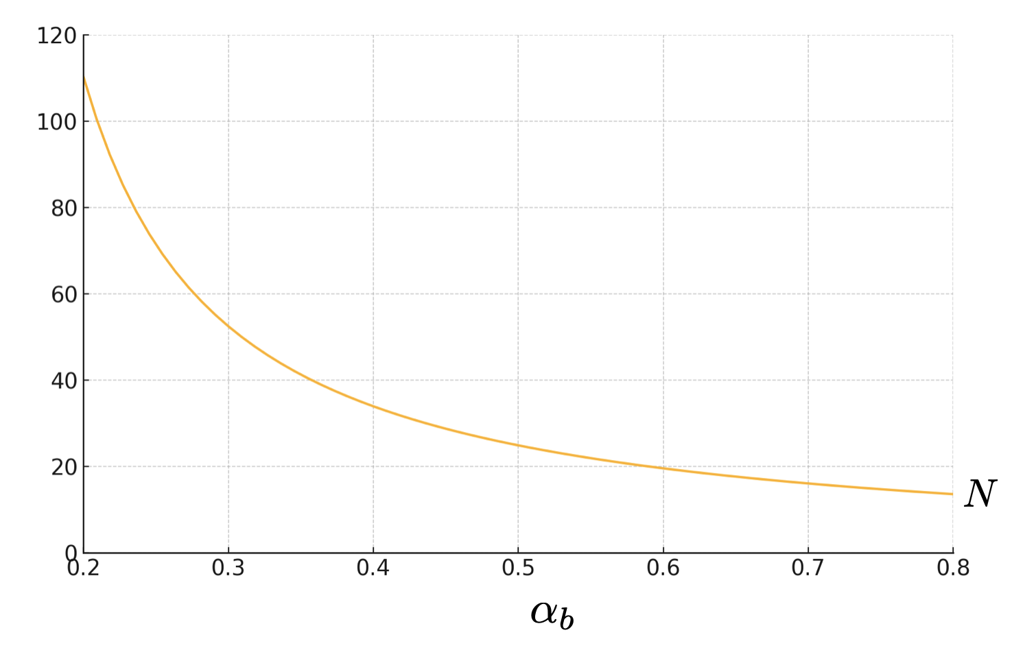
The comparisons in this theorem apply for reasonably small . For example, let , in which case the restriction in Assumption 3 is quite weak. Figure 1 fixes and plots for different values of . If (say), the human evaluator observes 10% of covariates while Black Box observes 90%, then the comparisons in Theorem 3.2 hold for all .
The case of convex (Part (a)) corresponds to a preference for more accurate evaluations.252525Consider any two sets of covariates and let , be the corresponding posterior expectations. The distribution of (i.e., the posterior expectation that conditions on more information) is a mean-preserving spread of the distribution of . When is convex, the former leads to a higher expected utility. Such an agent “prefers more accurate evaluations” in the sense that giving the evaluator better information (in the standard Blackwell sense) leads to an improvement in the agent’s expected utility. Such an agent prefers for the evaluation to be based on more information (advantaging Black Box), but also prefers for the evaluation to be based on more relevant covariates (advantaging Human). We show that what eventually dominates is how many covariates the evaluators observe, not how they are selected; for an agent who prefers accuracy, this favors the Black Box.
Part (b) of Theorem 3.2 says that if instead is concave, then the agent should eventually prefer the human evaluator. We conclude this section with example decision problems that induce utility functions satisfying the conditions of either part of the theorem.
Example 12.
Suppose the agent receives a dollar wage equal to the evaluation, and is risk averse in money. Then his utility function is for some increasing and concave , and Part (a) of Theorem 3.2 says that the agent prefers to be evaluated by the human.
Example 13.
Suppose the agent’s type is , and the evaluator chooses an action based on the observed covariates. The evaluator and agent share the utility function . The evaluator’s optimal action is , and the agent’s expected payoff given this action is
where is convex. So Part (a) of Theorem 3.2 says that the agent eventually prefers evaluation by the black box evaluator. Although the conditions of Theorem 3.2 are no longer met when is not binary, we show in Appendix A.7 that the conclusion of Part (a) of Theorem 3.2 generalizes for arbitrary given the mean-squared error payoff function described in this example.
4 Extensions
We now show that we are able to strengthen our main results (Theorems 3.1 and 3.2) in the following ways. In Section 4.1, we show that not only does the expected value of context vanish for each individual agent, but in fact the expected maximum value of context across agents also vanishes. That is, in expectation the most that context can benefit any agent in the population is small. From this, it is immediate that our main results also extend in a generalization of our model in which the agent has uncertainty over his covariate vector. In Section 4.2, we show that our main results extend when the agent and evaluator interact in a disclosure game, wherein the evaluator updates his beliefs to the agent’s strategic choice of what to disclose.
4.1 Max value of context across agents
So far we have studied the the expected value of context for a single agent. If we instead ask whether the firm should use human or algorithmic evaluation—for example, whether a hospital should automate diagnoses or rely on doctor evaluations—other statistics may also be relevant. For example, it may matter whether the value of context is large for any agent in the population (e.g., because a lawsuit regarding algorithmic error may be brought on the basis of harm to any specific individual (Jha, 2020)). We thus study the expected maximum value of context, as defined below.
Definition 4.1.
For any , the expected maximum value of context is
The following corollary says that this quantity also vanishes as grows large.
Corollary 1.
4.2 Strategic Disclosure
So far we’ve remained agnostic as to whether the agent or evaluator chooses which nonstandard covariates are revealed, assuming that in either case the evaluator updates as if the covariates were revealed exogenously. We now consider a more traditional disclosure game, in which the agent chooses which nonstandard covariates are revealed, and the human evaluator updates her beliefs about the agent’s type in part based on which covariates are chosen.
For any fixed function , call the following an -context disclosure game: There are two players, the agent and the evaluator. The function is common knowledge.262626We do not interpret this assumption literally. At the other extreme where is unknown to the agent, there is no informational content in which covariates the agent chooses to reveal, as they are all symmetric from the agent’s point of view. The set of possible disclosures is the set of all pairs consisting of a set of nonstandard covariates and values for those covariates. A disclosure is feasible for an agent with covariate vector if the disclosed covariate values are truthful, i.e., for every .
The agent chooses a disclosure strategy, which is a map
from covariate vectors to feasible disclosures. The agent then privately observes his covariate vector and discloses . The evaluator observes this disclosure and chooses an action . That is, the evaluator’s strategy is a function . The evaluator’s payoff is and the agent’s payoff is some function .
In this section we focus on pure strategy Perfect Bayesian Nash equilibria (PBE) of this game, henceforth simply equilibria. (A similar result holds for mixed strategy equilibria, which is demonstrated in the appendix.)
Definition 4.2.
Let denote the highest payoff that an agent with covariate vector receives in any pure-strategy equilibrium of the -context disclosure game. The expected maximum value of context disclosure is
We show that the best payoff that an agent can receive in any pure strategy -context equilibrium is bounded above by the maximum value of context across agents.
5 Relaxing our Assumptions on the Prior
As shown in Example 11, our main results can fail if the assumption of symmetric uncertainty over the role of the nonstandard covariate values (Assumption 1) is broken. We now propose two relaxations of Assumption 1 and one relaxation of Assumption 2, and explore the extent to which our main result extends. In Section 5.1, we suppose that it is known ex-ante that some covariates are relevant, while the remaining are not, so that even as grows to infinity, the effective number of covariates potentially grows more slowly. In Section 5.2 we allow the agent to have prior knowledge about the role of certain nonstandard covariates. In Section 5.3, we consider a model in which the predictability of the agent’s type is increasing in the total number of covariates. Finally, Section 5.4 provides an abstract condition on the learning environment under which our main results hold, which requires the evaluator’s uncertainty about the agent’s type to grow sufficiently fast in .
5.1 Not all covariates are relevant
Under Assumption 1, it cannot be known ex-ante that some covariates are irrelevant for predicting the type. The assumption thus rules out settings such as the following.
Example 14.
The evaluator is a job interviewer. Although in principle there is an infinite number of covariates that can describe a job candidate, it is understood that not all of them are actually relevant to the job candidate’s ability. That is, there is some potentially large (but not exhaustive) set of covariates that contain all of the predictive content about the candidate’s ability, and the remaining covariates are either irrelevant for predicting ability, or are predictive only because they correlate with other intrinsically predictive covariates.
If irrelevant covariates cannot be disclosed to the evaluator, then we return to our main model with a smaller and our previous results extend directly. The more novel case is the one in which it is known that covariates are irrelevant, but those covariates can still be disclosed to the evaluator (for example, because it is not commonly understood that they are irrelevant).272727To see the difference, consider the case in which the agent simply wants the evaluator to hold a higher posterior expectation. The irrelevant covariates create noise, and for some realizations of it may be that disclosing an irrelevant covariate leads to a higher evaluation.
To model this, we suppose there is a sequence of sets of relevant covariates such that each includes the standard covariates in and is of size , where is the (known) number of relevant nonstandard covariates. We will moreover without loss index these sets so that the relevant covariates are . The irrelevance of the remaining covariates is reflected in the following assumption, which says that, holding fixed the values of the relevant covariates, the values of the irrelevant covariates do not change the type.
Assumption 4 (Irrelevance).
There is a function such that
for every .
Assumption 5 (Exchangeability).
For every realization of , the sequence
| (5.1) |
is finitely exchangeable.
Assumption 6 (Constant Unpredictability of ).
For every realization of the standard covariates and every pair , the sequence and the truncated sequence are identical in distribution.
Our main model is otherwise unchanged—in particular, we allow the agent to disclose any of the nonstandard covariates, including those which are irrelevant. We show that our previous results extend so long as .
Proposition 5.1.
The case where (violating the assumption of the result) corresponds to a setting in which the number of relevant covariates is so small that the agent can disclose all of them. For example, if a job candidate is convinced that only 10 nonstandard covariates are actually relevant for predicting his on-the-job ability, and all of these nonstandard covariates can be shared during a job interview, then our main results do not extend and we should think of the value of context as being potentially large. On the other hand, if the set of relevant covariates are low-dimensional relative to the total number of covariates, but are still too numerous to be fully revealed, then our main results do extend.
This result suggests that whether human or black box evaluation is more appropriate should be determined in part based on whether the available signal is concentrated in a small number of covariates (favoring the human evaluator) or spread out across a large number of covariates (favoring the black box evaluator). The same application may transition between these regimes over time. For example, in a medical setting where black box diagnosis is highly accurate based on non-interpretable features of an image scan, it may not be possible to communicate sufficient information via any small number of covariates. But if the predictive features of the image are subsequently better understood and defined, then it may be that a small set of (newly defined) features does eventually capture all of the signal content, and can be fully disclosed in a conversation.
5.2 Certain nonstandard covariates have known effects
Another possibility is that the agent knows how certain nonstandard covariates are correlated with the type.
Example 15.
The agent is a patient who resided around Chernobyl at the time of the Chernobyl nuclear disaster of 1986. The agent is being evaluated for potential thyroid conditions, and knows that this particular part of his history increases the probability of a thyroid condition.
Specifically suppose there is a set of covariate indices whose effects are known. The set includes the standard covariates, but possibly also includes some nonstandard covariates. Without loss, we can index these . We weaken Assumption 1 to the following:
Assumption 7 (Exchangeability).
For every realization of the covariates ,
| (5.2) |
is finitely exchangeable.
This assumption imposes exchangeability only over the nonstandard covariates whose effects are not ex-ante known. Clearly if is a strict superset of , then the expected value of context need not vanish under Assumptions 2 and 7. A simple example is the following.
Example 16.
Suppose there are no standard covariates, and , i.e., the first nonstandard covariate has a known effect, where if and if . Suppose further that the agent’s covariate vector satisfies . Then the prior expectation of the agent’s type is 0, but revealing moves the posterior expectation to . So the expected value of context does not vanish.
But if we modify the definition in (2.2) to
with replacing , and again let , then the modified expected value of context
evaluates the value of context beyond those covariates with known effects. The same proof shows that this expected value of context vanishes to zero as grows large. That is, beyond the value of context that is already clear to the agent based on private knowledge about his nonstandard covariates, the agent does not expect substantial additional gain from the remaining covariates.
5.3 Information accumulates in
So far we have assumed that the predictability of is constant in the number of covariates. This is not essential for our results. Suppose instead that
where is a mean-zero random variable that is independent of the covariates . This describes a setting in which the covariates are not sufficient to reveal the agent’s type, and there is a residual unknown.
Our previous results extend directly when the distribution of is the same for all . Another natural case is one in which decreases monotonically in , with ; that is, in environments with a larger number of covariates, the agent’s type is more predictable. In Appendix B.5 we show that Theorem 3.1 directly extends. We also show that the comparisons in parts (a) and (b) of Theorem 3.2 hold for sufficiently large , under the following assumption:
Assumption 8.
For each , let and assume that admits a pdf, which we denote by . The sequence is bounded.
Loosely speaking, our comparisons in Theorem 3.2 continue to hold so long as the variance of does not increase too fast in .
5.4 Sufficient residual uncertainty
In this final section, we provide an abstract condition on the evaluator’s learning environment, under which Theorem 3.1 extends.
For each , let denote the set of all disclosures respecting the human evaluator’s capacity constraint, i.e., all pairs consisting of a set with or fewer nonstandard covariates, and values for those covariates. Further define to be the set of all disclosures. Similarly, for each let be the set of all type functions , and define . An evaluation rule is any family where each maps disclosures into evaluations for the given function . Finally, fixing any update rule , number of covariates , and disclosure , let
be the random evaluation when is drawn from according to the agent’s prior.
We impose two assumptions below on the evaluation rule. The first says that the expected evaluation is equal to the prior expected type ; the second says that the distribution of the evaluation concentrates on sufficiently fast as the number of hidden covariates grows large. Intuitively, the assumption requires that as the number of residual unknowns—i.e., the covariates which are predictive of the type, but are not revealed to the evaluator—grows large, the informativeness of any fixed disclosure becomes small.282828In the limit with an uninformative disclosure, the distribution of the evaluation is degenerate at the prior expectation for any Bayesian updating rule.
Assumption 9 (Unbiased).
for every disclosure .
Assumption 10 (Fast Concentration).
For any sequence of feasible disclosures ,
where is the number of unique sets with or fewer elements.
These assumptions do not in general represent a weakening of our main model. Previously we studied the evaluation rule mapping each disclosure into the conditional expectation of the agent’s type, and imposed Assumption 1 on the agent’s prior about . In this model, the evaluation for any disclosure could be represented as a sample average consisting of elements. Assumption 9 is clearly satisfied (because the update rule is Bayesian), but one can select a sequence of disclosures such that (see the proof of Theorem 3.1 for details). Thus the speed of convergence demanded in Assumption 10 is not met when is sufficiently large.
Nevertheless, Assumption 10 identifies the qualitative property of our main setting that gave us Theorem 3.1: residual uncertainty must have the power to overwhelm any information revealed through disclosure. Under these assumptions, our main result extends.
Proposition 5.2.
This result also clarifies that neither the precise symmetry imposed by Assumption 1, nor the assumption of Bayesian updating in our main model, are crucial for our main result.
6 Conclusion
One argument against replacing human experts with algorithmic predictions is that no matter how many covariates are taken as input by the algorithm, the number of potentially relevant circumstances and characteristics is still more numerous. In cases where some important fact is missed by a human evaluator, it is often possible to correct this oversight. There is no such safety net with a black box algorithm.
This is a compelling narrative, yet our results suggest that it may be less important than it initially seems. When there is a large number of nonstandard covariates that may matter for the prediction problem, but the agent does not know how these nonstandard covariates impact the type, then the expected value of disclosing additional information is small—even when we assume that the agent can identify the most useful covariates to disclose, and that the claims about these covariates are taken at face value.
In contrast, if the agent has substantial prior knowledge about the predictive roles of the nonstandard covariates, then our conclusion will not be appropriate. In particular, if there is a “low-dimensional” set of covariates that predict the type and can be fully disclosed (as in Example 9), or if there is a known structural relationship between covariates and the type (as in Example 11), then the expected value to disclosing additional information may be large. We thus view our results as revealing a link betwen the value of targeting information acquisition (beyond simply conditioning on large quantities of information) and the extent of prior “structural information” about the numerous covariates that can be brought up as explanations.
We conclude with two alternative interpretations of our model and results.
Online versus offline learning. In our model, a key distinction between human and black box evaluation is that the human can adapt which covariates are acquired based on other properties of the agent, while the black box cannot. This is an appropriate comparison of human and black box evaluators as they currently stand: The black box algorithms used to make predictions about humans are usually supervised machine learning algorithms which are pre-trained on a large data set. But new black box algorithms, such as large language models, blur this distinction, and future evaluations (e.g., medical diagnoses) may be conducted by black box systems with which the agent can communicate.
From this more forward-looking perspective, our results can be understood as comparing the merits of online versus offline learning. That is, how valuable is it to have the evaluator dynamically acquire information given feedback from the agent? Our result suggests that this is not important in expectation. For example, Part (a) of Theorem 3.2 implies that an agent who cares about accuracy should prefer a supervised machine learning algorithm trained on a large number of covariates over a conversation with ChatGPT that reveals a smaller number of covariates.
Value of human supervision of algorithms. While we have interpreted the standard covariates as a small set of covariates acquired by the human evaluator, an alternative interpretation is that they are the initial inputs to an algorithm. In this case, the expected value of context quantifies the sensitivity of the algorithm’s predictions to the addition of further relevant inputs, e.g., as identified by a human manager. This interpretation is particularly relevant when we consider accuracy as the objective, in which case the value of context tells us how wrong the algorithm is compared to if the algorithm could be retrained on additional relevant inputs. Theorem 3.1 says that while in certain cases additional inputs would lead to a substantially more accurate prediction, under our symmetry assumption on the agent’s prior this will not typically be the case.
References
- Acemoglu et al. (2015) Acemoglu, D., V. Chernozhukov, and M. Yildiz (2015): “Fragility of Asymptotic Agreement under Bayesian Learning,” Theoretical Economics, 11, 187–225.
- Acosta et al. (2022) Acosta, J., G. Falcone, P. Rajpurkar, and E. Topol (2022): “Multimodal biomedical AI,” Nature Medicine, 28, 1773–1784.
- Agarwal et al. (2023) Agarwal, N., A. Moehring, P. Rajpurkar, and T. Salz (2023): “Combining Human Expertise with Artificial Intelligence: Experimental Evidence from Radiology,” Working Paper 31422, National Bureau of Economic Research.
- Akbarpour et al. (2024) Akbarpour, M., S. Malladi, and A. Saberi (2024): “Just a Few Seeds More: Value of Network Information for Diffusion,” Working Paper.
- Angelova et al. (2022) Angelova, V., W. Dobbie, , and C. S. Yang (2022): “Algorithmic Recommendations and Human Discretion,” Working Paper.
- Antic and Chakraborty (2023) Antic, N. and A. Chakraborty (2023): “Selected Facts,” Working Paper.
- Arnold and Groeneveld (1979) Arnold, B. C. and R. A. Groeneveld (1979): “Bounds on expectations of linear systematic statistics based on dependent samples,” The Annals of Statistics, 220–223.
- Bardhi (2023) Bardhi, A. (2023): “Attributes: Selective Learning and Influence,” Working Paper.
- Bastani et al. (2022) Bastani, H., O. Bastani, and W. P. Sinchaisri (2022): “Improving Human Decision-Making with Machine Learning,” .
- Berman (1964) Berman, S. M. (1964): “Limit Theorems for the Maximum Term in Stationary Sequences,” The Annals of Mathematical Statistics, 35, 502 – 516.
- Blackwell and Dubins (1962) Blackwell, D. and L. Dubins (1962): “Merging of Opinions with Increasing Information,” The Annals of Mathematical Statistics.
- Chalfin et al. (2016) Chalfin, A., O. Danieli, A. Hillis, Z. Jelveh, M. Luca, J. Ludwig, and S. Mullainathan (2016): “Productivity and Selection of Human Capital with Machine Learning,” American Economic Review, 106, 124–27.
- Chernozhukov et al. (2013) Chernozhukov, V., D. Chetverikov, and K. Kato (2013): “Gaussian approximations and multiplier bootstrap for maxima of sums of high-dimensional random vectors,” .
- Crawford and Sobel (1982) Crawford, V. P. and J. Sobel (1982): “Strategic information transmission,” Econometrica: Journal of the Econometric Society, 1431–1451.
- Di Tillio et al. (2021) Di Tillio, A., M. Ottaviani, and P. N. Sørensen (2021): “Strategic Sample Selection,” Econometrica, 89, 911–953.
- Dworczak and Martini (2019) Dworczak, P. and G. Martini (2019): “The Simple Economics of Optimal Persuasion,” Journal of Political Economy, 127, 1993–2048.
- Dye (1985) Dye, R. A. (1985): “Disclosure of Nonproprietary Information,” Journal of Accounting Research, 23, 123–145.
- Farina et al. (2023) Farina, A., G. Frechette, A. Lizzeri, and J. Perego (2023): “The Selective Disclosure of Evidence: An Experiment,” Working Paper.
- Frankel (2014) Frankel, A. (2014): “Aligned Delegation,” American Economic Review, 104, 66–83.
- Frick et al. (2023) Frick, M., R. Iijima, and Y. Ishii (2023): “Learning Efficiency of Multiagent Information Structures,” Journal of Political Economy, 131, 3377–3414.
- Gillis et al. (2021) Gillis, T., B. McLaughlin, and J. Spiess (2021): “On the Fairness of Machine-Assisted Human Decisions,” Working Paper.
- Glazer and Rubinstein (2004) Glazer, J. and A. Rubinstein (2004): “On optimal rules of persuasion,” Econometrica, 72, 1715–1736.
- Golub and Jackson (2012) Golub, B. and M. Jackson (2012): “How Homophily Affects the Speed of Learning and Best-Response Dynamics,” The Quarterly Journal of Economics, 127, 1287–1338.
- Grossman and Hart (1980) Grossman, S. J. and O. D. Hart (1980): “Disclosure Laws and Takeover Bids,” The Journal of Finance, 35, 323–334.
- Haghtalab et al. (2021) Haghtalab, N., M. Jackson, and A. Procaccia (2021): “Belief polarization in a complex world: A learning theory perspective,” PNAS, 118, 141–73.
- Harel et al. (2020) Harel, M., E. Mossel, P. Strack, and O. Tamuz (2020): “Rational Groupthink*,” The Quarterly Journal of Economics, 136, 621–668.
- Hoffman et al. (2017) Hoffman, M., L. B. Kahn, and D. Li (2017): “Discretion in Hiring*,” The Quarterly Journal of Economics, 133, 765–800.
- Jha (2020) Jha, S. (2020): “Can you sue an algorithm for malpractice? It depends,” .
- Jin et al. (2021) Jin, G. Z., M. Luca, and D. Martin (2021): “Is No News (Perceived As) Bad News? An Experimental Investigation of Information Disclosure,” American Economic Journal: Microeconomics, 13, 141–73.
- Jung et al. (2017) Jung, J., C. Concannon, R. Shroff, S. Goel, and D. G. Goldstein (2017): “Simple rules for complex decisions,” Working Paper.
- Jussupow and Heinzl (2020) Jussupow, Ekaterina; Benbasat, I. and A. Heinzl (2020): “Why are we averse towards algorithms? A comprehensive literature review on algorithm aversion,” in In Proceedings of the 28th European Conference on Information Systems.
- Kamenica and Gentzkow (2011) Kamenica, E. and M. Gentzkow (2011): “Bayesian Persuasion,” American Economic Review, 101, 2590–2615.
- Klabjan et al. (2014) Klabjan, D., W. Olszewski, and A. Wolinsky (2014): “Attributes,” Games and Economic Behavior, 88, 190–206.
- Kleinberg et al. (2017) Kleinberg, J., H. Lakkaraju, J. Leskovec, J. Ludwig, and S. Mullainathan (2017): “Human Decisions and Machine Predictions,” The Quarterly Journal of Economics, 133, 237–293.
- Kushilevitz and Nisan (1996) Kushilevitz, E. and N. Nisan (1996): Communication Complexity, Cambridge University Press.
- Lai et al. (2023) Lai, V., C. Chen, A. Smith-Renner, Q. V. Liao, and C. Tan (2023): “Towards a Science of Human-AI Decision Making: An Overview of Design Space in Empirical Human-Subject Studies,” in Proceedings of the 2023 ACM Conference on Fairness, Accountability, and Transparency, New York, NY, USA: Association for Computing Machinery, FAccT ’23, 1369–1385.
- Liang and Mu (2019) Liang, A. and X. Mu (2019): “Complementary Information and Learning Traps*,” The Quarterly Journal of Economics, 135, 389–448.
- Liang et al. (2022) Liang, A., X. Mu, and V. Syrgkanis (2022): “Dynamically Aggregating Diverse Information,” Econometrica, 90, 47–80.
- Longoni et al. (2019) Longoni, C., A. Bonezzi, and C. K. Morewedge (2019): “Resistance to Medical Artificial Intelligence,” Journal of Consumer Research, 46, 629–650.
- McLaughlin and Spiess (2022) McLaughlin, B. and J. Spiess (2022): “Algorithmic Assistance with Recommendation-Dependent Preferences,” Working Paper.
- McLean and Postlewaite (2002) McLean, R. and A. Postlewaite (2002): “Informational Size and Incentive Compatibility,” Econometrica, 70, 2421–2453.
- Milgrom (1981) Milgrom, P. R. (1981): “Good News and Bad News: Representation Theorems and Applications,” The Bell Journal of Economics, 12, 380–391.
- Morris and Yildiz (2019) Morris, S. and M. Yildiz (2019): “Crises: Equilibrium Shifts and Large Shocks,” American Economic Review, 109, 2823–54.
- Obermeyer and Emanuel (2016) Obermeyer, Z. and E. J. Emanuel (2016): “Predicting the Future - Big Data, Machine Learning, and Clinical Medicine,” The New England Journal of Medicine, 375, 1216–9.
- Raghu et al. (2019) Raghu, M., K. Blumer, G. Corrado, J. Kleinberg, Z. Obermeyer, and S. Mullainathan (2019): “The Algorithmic Automation Problem: Prediction, Triage, and Human Effort,” Working Paper.
- Rajpurkar et al. (2017) Rajpurkar, P., J. Irvin, K. Zhu, B. Yang, H. Mehta, T. Duan, D. Ding, A. Bagul, C. Langlotz, K. Shpanskaya, M. P. Lungren, and A. Y. Ng (2017): “CheXNet: Radiologist-Level Pneumonia Detection on Chest X-Rays with Deep Learning,” Working Paper.
- Spiegler (2020) Spiegler, R. (2020): “Behavioral Implications of Causal Misperceptions,” Annual Review of Economics, 12, 81–106.
- Vives (1992) Vives, X. (1992): “How Fast do Rational Agents Learn?” Review of Economic Studies, 60, 329–347.
- Yang et al. (2024) Yang, K. H., N. Yoder, and A. Zentefis (2024): “Explaining Models,” Working Paper.
Appendix A Proof of Generalization of Theorem 3.1
In a change of notation relative to the main text, we subsequently use to denote the agent’s covariate vector and to denote the agent’s type (leaving and to denote realizations of these random variables). Moreover, rather than supposing that is deterministically related to via a function , let where is unknown. We replace Assumptions 1 and 2 with the following weaker assumption.
Assumption 11.
Fix any realization of the standard covariates . There is an infinitely exchangeable sequence such that for every , the sequence
has the same distribution as .
That is, permuting the labels and/or values of the nonstandard covariates does not change the joint distribution of the conditional expectations of . When is degenerate conditional on , Assumption 11 reduces to our previous two assumptions. We will prove the following generalization of Theorem 3.1.
Theorem A.1.
Suppose Assumption 11 holds. Then for every covariate vector , the expected value of context vanishes to zero as grows large, i.e., .
Towards this, we will first prove the conclusion under a strengthening of Assumption 11, where exchangeability is replaced by an assumption that conditional expectations are i.i.d. across the different possible completions of the agent’s covariate vector.
Assumption 12.
Fix any realization of the standard covariates . Then there is a distribution such that for every , the conditional expectations
across all vectors .
Theorem A.2.
Suppose Assumption 12 holds. Then for every covariate vector , the expected value of context vanishes to zero as grows large, i.e., .
A.1 Outline for Proof of Theorem A.2
Fix any realization of the agent’s standard covariates. After observing , the evaluator assigns positive probability to the covariate vectors whose first entries are equal to . Let these covariate vectors be indexed by where , and define
to be the (random) expected type given covariate vector . By assumption that the marginal distribution over covariate vectors is uniform, the evaluator’s posterior expectation of the agent’s type after observing the agent’s standard covariates is
There are subsets of that contain or fewer elements. Enumerate these sets as . For each , let
be the set of indices for those covariate vectors that agree with the agent’s covariate vector in entries (where is as defined in (2.1)). After observing the agent’s nonstandard covariates in the set , the evaluator’s posterior expectation about the agent’s type is
Although the distributions of the random variables vary across , we suppress this dependence in what follows to save on notation. The remainder of the proof proceeds by first showing that in expectation the possible increase in the evaluator’s posterior expectation over the prior expectation is vanishing.
Proposition A.1.
This is subsequently strengthened to the statement that the expected maximum absolute difference between and converges to zero.
Proposition A.2.
And finally we apply the above proposition to demonstrate the conclusion of the theorem, i.e., that
Thus in expectation the possible increase in the agent’s payoff also vanishes. We suppress dependence of on the covariate vector in what follows, writing simply .
A.2 Proof of Proposition A.1
Statement of the proposition:
The quantity is the expected first-order statistic of a sequence of non-i.i.d. variables . The proof is organized as follows. In Sections A.2.1 and A.2.2, we define i.i.d. variables with the property that
| (A.1) |
In Sections A.2.3 and A.2.4, we show that the RHS of the above display converges to as grows large.
A.2.1 Replacing ’s with independent variables
In general, disclosures and may lead to posterior expectations and that are correlated due to the presence of the same ’s across the different sample averages. We first show that replacing these ’s with properly defined independent random variables weakly increases the value of context.
Definition A.1.
For each define
| (A.2) |
where , so that each has the same distribution as , but the vector is mutually independent.
Lemma A.1.
Let
and
Then for all .
Proof.
Throughout we use to mean that the distribution of first-order stochastically dominates the distribution of .
Sublemma 1.
Let ,…, , be a sequence of real-valued random variables (not necessarily i.i.d.). Let be a sequence of positive constants. Further, let be i.i.d. random variables, independent of . Define
Then and .
Proof.
For define:
so that is the maximum of the first terms in , and replaces in the -th term of with . We first demonstrate an analogue of the desired conclusions for and .
Sublemma 2.
and .
Proof.
Without loss of generality set . We’ll first show that . To establish first-order stochastic dominance, we need to show that for all it holds that
For each define the event
Further let
be the event that achieves the maximum among . We’ll show that the FOSD rankings in Sublemma 2 hold both on event and also on its complement .
Define
to be the event that achieves the maximum among . Then
Thus .
Now consider the event , on which does not achieve the maximum among . Then either , in which case , or , in which case . So
and hence .
Now we show that . For any realization of , let denote the conditional random variable . Define and identically to and , replacing each by . Then by independence of and , the distribution of is identical to that of , and the distribution of is identical to that of .
Applying the first part of this sublemma to and , we conclude that . Since is an increasing convex function, it preserves the first-order stochastic dominance relation and hence . This argument holds pointwise for all so as desired. ∎
Finally, we use Sublemma 1 to establish Lemma A.1, i.e., the expected value of context weakly increases if we make the ’s within different disclosures independent. We will prove this iteratively. For arbitrary , define the random variable
Fix any . We will show that replacing across different sample averages with independent copies of this random variable leads to a FOSD increase in the distribution of .
Let be the set of indices of sample averages which contain . Then we can rewrite the previous display as
or
| (A.3) |
where for each , and . Because are mutually independent, is independent of each and . So applying Lemma 1, the random variable in (A.3) has a distribution that is first-order stochastically dominated by the distribution of
as desired. Since is arbitrary, this concludes the proof.
∎
A.2.2 Replacing with i.i.d. Variables
The variables are sample averages of unequal sizes ranging between and elements. We next show that replacing each of these variables with a sample average of elements (the smallest size) weakly increases the value of context.
Definition A.2.
For each define
| (A.4) |
to be the analogue of with elements instead of , so that the variables are iid.
Lemma A.2.
Let
Then for all .
Proof.
We use the following result.
Sublemma 3.
Suppose are independent and identically distributed random variables, and define to be their sample average. Let and define . Then the distribution of is a mean preserving spread of the distribution of .
Proof.
First observe that for any , since
where the final equality follows by assumption that the ’s are iid. Then
and the distribution of is a mean-preserving spread of the distribution of as desired. ∎
This lemma implies that each second-order stochastically dominates (since for all ). The desired result then follows by Jensen’s inequality, since the entries of are (by construction) independent and the maximum is a convex function. ∎
A.2.3 Asymptotic Normality
Lemma A.3.
Let
where . Then
Proof.
Without loss of generality, let .292929If , the statement of Theorem 3.1 holds trivially. First observe that
where each
Similarly we can write
where each
When the assumptions for Corollary 2.1 from Chernozhukov et al. (2013) are met (to be verified momentarily), we can conclude that
where denotes Kolmogorov distance. Thus also
| (A.5) |
where
By assumption, each is supported on for some finite . This implies for all , so the sequence is uniformly integrable. The convergence in (A.5) thus implies
as desired.
It remains to verify that the conditions of Corollary 2.1 from Chernozhukov et al. (2013) are met. This follows from the assumption that ’s are uniformly bounded, and the observation that
for any , since by the Binomial Theorem and . ∎
A.2.4 Upper Bound for Expected Maximum of Gaussians
A.3 Proof of Proposition A.2
Statement of the proposition:
In an abuse of notation, let denote de-meaned sample average. By rewriting the max within the expectation we obtain
We will show that each term of this final expression converges to zero. Observe that
| (A.6) |
Moreover,
so
| (A.7) |
From Lemma A.1,
| (A.8) |
Moreover, we showed in Section A.2.1 that the distribution of first-order-stochastically-dominates that of , so
which converges to zero as grows large since each . Finally,
| (A.9) |
uniformly across . Putting together (A.6) - (A.9) we have that
as desired. The argument that
follows identically, observing that Proposition A.1 is satisfied for , and that
A.4 Concluding the proof of Theorem A.2
Recall that denotes the (random) posterior expectation when the agent chooses not to disclose any nonstandard covariates. Clearly (since the agent can always choose to disclose nothing). Also
| (A.10) |
Each absolute difference can be bounded from above using the triangle inequality
| (A.11) |
A.5 Theorem A.2 implies Theorem A.1
In an abuse of notation, let mean that across all covariate vectors . We have already shown in Theorem 3.1 that for any distribution . Now suppose instead that Assumption 1 is satisfied. By de Finetti’s theorem, there exists a set , family of conditional measures , and measure such that
where the inner expectation converges to zero for every by Theorem A.2. By assumption that is Lipschitz continuous on a compact domain, there exist and such that for all . So is pointwise bounded above by , and the Dominated Convergence Theorem implies , as desired.
A.6 Proof of Theorem 3.2
Throughout the proof we set , and without loss of generality. We’ll start by demonstrating that the stated results hold asymptotically (i.e., for large enough ) and subsequently prove that the bound in (3.4) is sufficient.
(a) As before let index those covariate vectors that agree with the agent’s covariate vector for all covariates in . Then the black box evaluator’s posterior expectation is the sample average
We will show that
for large enough .
We start by analyzing the first difference . Using Taylor’s expansion we get
for some . Note that . Moreover, for some , since is strictly convex. Thus
| (A.14) |
Next turn to . For each term inside the maximum we have that
| (A.15) |
where the latter inequality follows from the fact that is continuous on a compact set, and hence bounded by some . Thus
Combining the bounds from steps 1 and 2 we get
The RHS is positive for all large if and only if
since has sub-exponential but non-constant asymptotics. This condition is satisfied if and only if .
(b) Since is convex, the above arguments apply to show that
for some , while
for some . The desired conclusion follows.
Finally, we show that the bound in (3.4) is sufficient for the comparison in part of the result (with identical computations applying to part ). Suppose is strictly convex and denote , where are the constants used above, respectively reflecting ’s lowest degree of convexity () and largest growth rate (). Following the proof of part (a), the Black Box is preferred if
Since , this inequality is satisfied if
The above inequality implicitly defines a threshold on the sufficient number of covariates , exceeding which the Black Box is preferred.
A.7 Result Extending Theorem 3.2 Part (a)
Consider a model in which the evaluator chooses an action given the realization of the agent’s covariates, and the evaluator and agent share the payoff function . The following result shows that the conclusion of Part (a) of Theorem 3.2 extends for non-binary types .
Proposition A.3.
There exists an sufficiently large such that the agent prefers the black box evaluator for all .
Proof.
Throughout the proof set , and without loss. We will show that
for large enough .
Let denote the covariates that Black Box observes, and as before let denote Black Box’s (random) posterior expectation. The optimal action choice yields expected payoff . By the Law of Total Variance, . Since additionally , we obtain
Now turn to . By Lipschitz continuity of , there is a constant such that holds pointwise for each realization of . So
The remainder of the proof proceeds identically to the proof of Theorem 3.2. ∎
Appendix B Proofs for Results in Sections 4 and 5
B.1 Proof of Corollary 1
We continue in the general setting outlined in the proof of Theorem A.1. Fix any realization of the standard covariates. As in the proof of Theorem 3.1, there are covariate vectors with positive probability conditional on . Index these by , and define
to be the expected type given covariate vector . For each covariate vector and each disclosure set , there is a corresponding set of covariate vectors such that the evaluator’s posterior expectation after the agent discloses his covariates in set is
Different from the proof of Theorem 3.1, there are now unique sets (ranging over not only the different possible sets of covariates to disclose but also their values). By the Binomial Theorem,
Following the proof of Lemma A.1, we obtain that
which again converges to zero by assumption that . Finally observe that
Since each as , the RHS converges to zero. We thus obtain the analogue of Lemma A.2 for the expected maximum value of context, and the remainder of the proof proceeds identically to Theorem 3.1.
B.2 Proof of Proposition 4.1
Throughout this proof, we set for simplicity of notation.
Let denote a typical PBE, where is the Sender’s disclosure strategy and is the Receiver’s belief function. Fixing any such equilibrium, we use to denote the Receiver’s posterior expectation given disclosure . We first prove that at least one pure-strategy equilibrium always exists.
Proposition B.1.
For every n and f there exists a pure-strategy f-context equilibrium.
Proof.
Consider a candidate equilibrium , where for all (which is clearly a feasible disclosure for all agents). The Receiver’s beliefs at disclosure are pinned down by Bayes’ rule. For any other disclosure , we construct out-of-equilibrium beliefs such that . This is always possible, for example by setting for every . Then by construction reporting is a best response for any , so we are done. ∎
Consider any function and any pure-strategy equilibrium of the -context disclosure game. Let index the disclosures that have positive probability under (i.e., all such that for some ). For each such disclosure ,
is the evaluator’s posterior expectation upon observing disclosure . Given the evaluator’s payoff function, the optimal action for the evaluator is precisely . Let
| (B.1) |
be the disclosure that yields the highest payoff to the Sender. Then it must be that for every covariate vector for which disclosure is feasible. Otherwise would be a profitable deviation. Hence the evaluator’s posterior expectation in this equilibrium is the same as it would have been given disclosure of in our main model. So
Since the payoff received by an agent with any other covariate vector cannot exceed (by (B.1)), we have the desired result.
B.3 Result for Mixed Strategy Equilibria
In this part we restrict to equilibria with the property that is unique on the set of posterior expectations with positive probability in this equilibrium. Call these equilibria generic. (A sufficient condition for all equilibria to be generic is if is strictly monotone.)
For each and , let denote the highest payoff that an agent with covariate vector receives in any generic equilibrium (potentially mixed) of the -context disclosure game. Further define
and
where the expectation is with respect to the realization of .
Proposition B.2.
Suppose Assumption 1 holds and is twice continuously differentiable. Then .
Proof.
Fix , , and a context equilibrium of the -context disclosure game. Let be the compact set of all equilibrium posterior expectations that are realized with positive probability in this equilibrium. Further, denote
to be the most-preferred achievable posterior expectation, which is unique by assumption of genericity of the equilibrium.
Since is the best attainable posterior expectation, an agent achieves in equilibrium if and only if it is feasible. (Otherwise, the agent can profitably deviate to the feasible disclosure that induces this posterior expectation.)
Let denote the set of agents who have a feasible disclosure that achieves . Let be the set of disclosures that agents in send with positive probability in equilibrium. By the logic above, . Using the structure of this equilibrium we can write
| (B.2) |
where is the ex-ante probability that the agent’s covariate vector belongs to , and is the expectation of the agent’s type given that his covariate vector does not belong to . Here we utilize the fact that the evaluator’s posterior expectation is constant at across all agents with covariate vectors in .303030In general this does not have to be the case. We rule this out in the definition of the equilibrium.
Now, consider the following alternative “strategy” , which relaxes the feasibility constraint: For any let , i.e., the disclosures are the same as in the original equilibrium. Further choose some arbitrary disclosure and let for all . The Receiver’s posterior expectation following observation of disclosure is
and, analogous to (B.2), we can write
| (B.3) |
Combining equations (B.2) and (B.3) we conclude:
which almost surely converges to so long as . Since the ’s are uniformly bounded, this also implies , as desired. We now demonstrate that indeed .
For any disclosure denote by the set of all covariate vectors x given which is feasible. Since is achieved by all agents for whom is feasible, it must be that for every disclosure we have . Then for any ,
where the limit follows by assumption that . This completes the proof. ∎
B.4 Proof of Proposition 5.1
We again continue in the general setting outlined in the proof of Theorem A.1, and adopt the conventions that while . We prove the result for a weakening of Assumptions 5 and 6 to the following.
Assumption 13.
Fix any realization of the standard covariates . There is an infinitely exchangeable sequence such that for every , the sequence
has the same distribution as .
Recalling that is the number of relevant covariates, there are distinct expected conditional types, which we can enumerate as . If disclosure involves disclosing relevant covariates, then there is a set of size such that the evaluator’s posterior expectation can be written
As in Step 1 of the proof of Theorem 3.1 (Section A.2.1), replace each with a variable which is independent across disclosure sets. This yields the random variables
As in the proof of Proposition A.1, it follows from Lemma 1 that
Next define
and note that these are identically and independently distributed with shared variance
Following the arguments in Step 2 of the proof of Theorem 3.1 (Section A.2.2), we get
where as before . Further, by the argument given in Step 3 of the proof of Theorem 3.1 (Section A.2.3),
where
and . Again applying the bound from Berman (1964), we have
By assumption that , the right-hand expression converges to zero as grows large, concluding the proof.
B.5 Supporting Materials for Section 5.3
We show here that both main results generalize to the setting with noise. Instead of repeating the proof step by step, we emphasize what changes must be made in order for the proofs to translate. To be consistent with our previous notation, we again operate with where enumerates covariate vectors. In all subsequent notation a tilde will indicate an object that includes noise , and objects without one are the same as in the main text. Observe that after adding the noise term , the key objects from the proofs transform in the following way: is replaced by , and is replaced by . Since , the proof of Theorem 3.1 translates directly.
To demonstrate Theorem 3.2, we will show how to adjust the proof of part (a) with part (b) following analogously. The first change is that (A.14) becomes
The inequality in (A.15) is also modified to
for every disclosure . Thus we obtain
We will show that the ratio grows arbitrary large with , thus asymptotically exceeding . Fixing some and applying Markov inequality, we obtain
| (B.4) |
If we denote the CDF of as , the RHS of the above inequality can be rewritten as . As grows large, the term in brackets tends to . We will omit the term until the end of the proof.
Fix an arbitrary and let . Further, fix such that , where . Then since is decreasing and we have that for all
Combining this inequality with (B.4) we get
for all . Since is an arbitrary positive number, this concludes the proof.
B.6 Proof of Proposition 5.2
Throughout the proof we assume and . In addition, for simplicity of notation, we enumerate feasible disclosures by and denote the corresponding posteriors (as random variables) as . To upper bound the value of context, we apply a result from Arnold and Groeneveld (1979):
| (B.5) |
By Assumption 9, inequality B.5 simplifies to
Finally, Assumption 10 implies that for every disclosure . Hence
which yields the desired result after taking a limit in . The argument for the lower bound follows the same line of reasoning and is thus omitted.