The Synchrotron Polarization In Decaying Magnetic Field in Gamma-Ray Bursts

The MF configuration in the emission region of GRBs is unknown. A possibility is the MF is ordered on large scales, such as the toroidal MF, which comes from the GRB central engine. The field couples with the GRB jet material and is launched along with the jet. Due to the expanding of the jet, the MF strength in the jet comoving frame will decay with the jet radius. This will produce a harder spectrum than the fast cooling spectrum, which can explain the GRB spectra (UZ14). Consider a GRB comes from a thin shell moving with a bulk Lorentz factor of $\Gamma$. The MF strength can be described by (Spruit et al. 2001; UZ14)

where $R=R_{s}+\beta c\Gamma t^{\prime}$ is the jet radius, $R_{0}$ is the radius where the MF begins to decay, $R_{s}$ is the radius where the GRB emission starts, $B^{\prime}_{0}$ is the initial MF strength and $a$ is the MF decaying index. $a=0$ corresponds to the constant MF case.

In the GRB emission region, high-energy electrons mainly cool down by SYN, ADI and IC mechanisms. For an electron with energy of $\gamma^{\prime}_{e}$, the synchrotron cooling rate is given by (Rybicki & Lightman 1979)

The ADI cooling rate can be described as (e.g., Tavecchio et al. 2003; Uhm et al.2012)

The IC cooling rate is (Jones 1968; Böttcher et al. 1997; Finke et al. 2008; Yan et al. 2016)

where ${\cal G}(\gamma^{\prime}_{e},\nu^{\prime})$ are given by ${\cal G}(\gamma^{\prime}_{e},\nu^{\prime})=\displaystyle\frac{8}{3}\frac{E(1+5E)}{(1+4E)^{2}}-\frac{4E}{1+4E}(\frac{2}{3}+\frac{1}{2E}+\frac{1}{8E^{2}})+\textrm{ln}(1+4E)[1+\frac{3}{E}+\frac{3}{4}\frac{1}{E^{2}}\displaystyle+\frac{\textrm{ln}(1+4E)}{2E}-\frac{\textrm{ln}(4E)}{E}]-\frac{5}{2}\frac{1}{E}+\frac{1}{E}\sum_{n=1}^{\infty}\frac{(1+4E)^{-n}}{n^{2}}-\frac{\pi^{2}}{6E}-2$ for $E>1/4$, and ${\cal G}(\gamma^{\prime}_{e},\nu^{\prime})=\displaystyle E^{2}(\frac{32}{9}-\frac{112}{5}E+\frac{3136}{25}E^{2})$ otherwise. $E=\gamma^{\prime}_{e}h\nu^{\prime}/m_{e}c^{2}$ and $h$ is the Planck constant. Here we adopt a differet method from that of Geng18 in calculating the IC cooling rate. The method should be more efficient in numerical implementation because the dimension of integral is less. $u^{\prime}(\nu^{\prime})$ is the comoving photon energy density per unit frequency, and is given by

where $\gamma^{\prime}_{e,\textrm{m}}$ and $\gamma^{\prime}_{e,\textrm{max}}$ are the minimum and maximum electron Lorentz factors, respectively and $P^{\prime}(\gamma^{\prime}_{e},\nu^{\prime})$ is the spectral power (erg s^-1 Hz^-1) of the synchrotron emission in the comoving frame (Rybicki & Lightman 1979)

Here $x=\nu^{\prime}/\nu^{\prime}_{c}$, $\nu^{\prime}_{c}=\frac{3q_{e}B^{\prime}\sin\alpha^{\prime}}{4\pi m_{e}c}\gamma_{e}^{{}^{\prime}2}$, and $K_{5/3}(\xi)$ is the Bessel function, $\alpha^{\prime}$ is the pitch angle, i.e., the angle between the magnetic field and the electron velocity. $\Delta R^{\prime}\thickapprox R/\Gamma$ is the comoving width of the shell. $I^{\prime}(\nu^{\prime})$ and $j^{\prime}(\nu^{\prime})$ are the specific intensity and emission coefficient (Rybicki & Lightman 1979), respectively. $V^{\prime}=4\pi R^{2}\Delta R^{\prime}$ is the volume of the shell. The instantaneous electron distribution $dN^{\prime}_{e}/d\gamma^{\prime}_{e}$ can be obtained by solving the continuity equation of the electrons in energy space (e.g., Longair 2011; Zhao et al. 2014; UZ14; Geng18),

where $\dot{\gamma}^{\prime}_{e,\textrm{tot}}$ is the total cooling rate of the electrons, i.e., $\dot{\gamma}^{\prime}_{e,\textrm{tot}}=\dot{\gamma}^{\prime}_{e,\textrm{syn}}+\dot{\gamma}^{\prime}_{e,\textrm{adi}}+\dot{\gamma}^{\prime}_{e,\textrm{SSC}}$. $Q^{\prime}(\gamma^{\prime}_{e})=Q^{\prime}_{0}\gamma_{e}^{\prime-p}$ (for $\gamma^{\prime}_{m}<\gamma^{\prime}_{e}<\gamma^{\prime}_{\textrm{max}}$) is the electron injection term, which is assumed to be a power-law form.

The observed flux density is $F_{\nu}\simeq I^{\prime}(\nu^{\prime})\delta^{3}\Delta\Omega/(1+z)^{3}$, where $\Delta\Omega=\pi(R/\Gamma)^{2}/D_{A}^{2}=\pi R^{2}(1+z)^{4}/\Gamma^{2}D_{L}^{2}$ is the solid angle of the visible region seen from the observer, the comoving frequency is $\nu^{\prime}=(1+z)\nu/\delta$, z is the redshift and $D_{L}$ is the luminosity distance. Taking the approximation of Doppler factor $\delta$ in the visible angular range of $1/\Gamma$ as $\delta\approx\Gamma$ and using equation (6), we obtain

With this equation, we can calculate the flux density spectra.

Similar to what was done in Geng18, we consider three kinds of models with different cooling mechanisms, namely, M1 (only synchrotron cooling with the constant MF or $a=0$), M2 ( synchrotron and adiabatic coolings with $a=0.0,1.0,1.2,1.5$, corresponding to the model of UZ14) and M3 (synchrotron, adiabatic and SSC coolings with $a=0.0,1.0,1.2,1.5$, corresponding to M3 and M4 of Geng18). The detail model parameters used in our calculations are listed in Table 1- 3. The adopted parameters, such as $B^{\prime}_{0}$ and $\gamma^{\prime}_{m}$, are based on the constraint of observed spectral peak energy $E_{\textrm{peak}}=1/(1+z)\cdot 3hq_{e}B^{\prime}_{0}\Gamma\gamma_{m}^{\prime 2}/4\pi m_{e}c\sim 500\textrm{keV}$, where the on-axis case is assumed. The cosmological parameters ($\Omega_{m}=0.27$, $\Omega_{\lambda}=0.73$, $H_{0}$=71 km s${}^{-}1$ Mpc^-1) are used, and the redshift is set to be $z=1$.

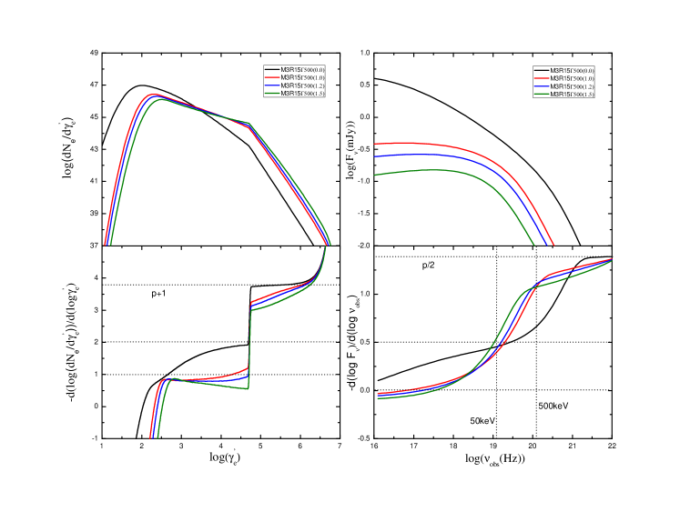
We solve the continuity equation of electrons in the energy space (Eq. 7). The fully implicit difference scheme proposed by Chang & Cooper (1970) and Chiaberge & Ghisellini (1999) is adopted. To test our code, we first use the same parameters as those in UZ14 and Geng18, and compare the resulting electron distributions and spectra. With the parameters listed in Table 1, we find our results are consistent with theirs (see Fig. 1 and 2). It needs to be noted that the initial MF strength in UZ14, where the GRB starts, is actually 300 G for $a=1$, not 30 G, because the MF begins to decay at $R_{0}=10^{14}$ cm while the GRB emission starts from $R_{s}=10^{15}$ cm in their model. In Fig. 3 and 4, like Geng18, we consider the case in which the two radii are equal. One can find the decaying MF indeed generates a harder spectrum in low-energy bands, similar to the Band spectrum. With the electron distribution we will calculate the PD.

In this section, we describe the method of calculating the polarization of synchrotron emission which with a large-scale order MF. A relativistic electron in the large-scale order MF will generate strong polarized synchrotron radiation. The spectral power of the electron can be divided into two different polarization states, i.e., (Rybicki & Lightman 1979)

where

and $\nu^{\prime}_{L}=q_{e}B/2\pi m_{e}c$ is the gyro-frequency. The synchrotron polarization from the electron can be calculated by (Rybicki & Lightman 1979)

For an electron population with a distribution of $dN^{\prime}_{e}/d\gamma^{\prime}_{e}$, the total polarization degree is

Consider the GRB jet has an half opening angle of $\theta_{j}$ and assume the jet is dominated by the toroidal magnetic field. The synchrotron polarization for a given observed frequency $\nu$ from the burst can be derived by calculating the Stokes parameters, i.e.,

where $\chi$ is the polarization position angle in the observer frame. $\nu^{\prime}=(1+z)\nu/\delta$ is the comoving frequency and $\delta=1/[\Gamma(1-\beta\cos\theta)]$ are the Doppler factor. For the given observed wavebands [$\nu_{1},\nu_{2}$], the degree of linear polarization of the jet emission is given by

where $t^{\prime}=t_{\textrm{obs}}\delta/(1+z)$ is the jet comoving time and $t_{\textrm{obs}}$ is the observed time. Note that $U=0$. Following Toma09, here we define several variables, $y\equiv(\Gamma\theta)^{2}$, $y_{j}\equiv(\Gamma\theta_{j})^{2}$, and $q\equiv\theta_{v}/\theta_{j}$, where $\theta_{v}$ is the viewing angle. $f$ is a function of $y$. During an observed GRB pulse, the polarization degree varies with time. We thus calculate the instantaneous and time-integrated polarizations over the pulse. The observed pulse can be generated when a thin relativistic shell emits photons within a radius range of $R_{s}$ to $R_{\textrm{off}}$, i.e., the emission starts at $R_{s}$ and turns off at $R_{\textrm{off}}$. Note that the turning off of the emission does not mean the observed emission sharply stops, because the higher latitude emission arrives at the observer at later time. Take the time when a testing photon emitted from the origin (the center of the GRB central engine) arrives at the observer as the observed time zero point. The starting times of the GRB pulse are $t_{\textrm{obs0}}=R_{s}(1+z)[1-\beta]/(\beta c)$ and $t_{\textrm{obs0}}=R_{s}(1+z)[1-\beta\cos(\theta_{v}-\theta_{j})]/(\beta c)$ for the on-axis and off-axis cases, respectively. The turn-off times of the GRB pulse are defined as $t_{\textrm{off}}=R_{\textrm{off}}(1+z)[1-\beta]/(\beta c)$ and $t_{\textrm{off}}=R_{\textrm{off}}(1+z)[1-\beta\cos(\theta_{v}-\theta_{j})]/(\beta c)$ for the on-axis and off-axis cases, respectively, where $R_{\textrm{off}}$ is set to be $R_{\textrm{off}}=10R_{\textrm{s}}$. For the time-integrated polarization, $f(y)=(1+y)^{-2}$ while for the instantaneous polarization, $f(y)=(1+y)^{-3}$ (Nakar & Piran 2003). Other variables can be described by (Toma09)

where $s=\theta/\theta_{v}$.

Fig. 5 shows the instantaneous polarization evolution and the corresponding normalized (normalized to the peak flux) light curves for the constant MF model of M1R14$\Gamma$300(0.0) (see Table 2 for detailed parameters) and for different viewing angles. Here we take the jet opening angle as a typical value of $0.1$ and all the PDs are calculated in the observed energy band of 50-500 keV, which is roughly the energy range of the current GRB polarimeters such as POLAR. Fig. 6 and 7 are for models M2 and M3 (constant and decaying MF models with different initial radii), respectively. One can find generally the PDs in various models for both the on-axis and off-axis cases have similar behaviors, i.e., they first decrease steeply at the beginning, then approximately remain a constant (plateau) before the turn-off time $t_{\textrm{off}}$ and decrease rapidly after $t_{\textrm{off}}$, except that in Fig. 6 and 7, there is a rising at the very beginning. It is also noted that the PD evolution is nearly independent of the initial radius and that the off-axis PD decreases with the increase of the viewing angle.

The PD curves are different in details (see Fig. 5, 6 and 7). The off-axis PD is higher than the on-axis PD at the beginning of the pulse. This can be understood as follows. In the very early phase, the polarization is approximately the local physical polarization since only a very tiny angular region is observed and the MF can be seen as parallel lines. The intrinsic energy band contributing to the given observed band would be higher in the off-axis case than in the on-axis case due to the Doppler effect. So at an early time, the off-axis PD can be from the -p/2 spectral segment of the synchrotron emission and thus is as large as $\sim 0.78$ (p=2.8), while the on-axis PD is from the combination of 1/3 and -1/2 spectral segments and is in the range of $0.5-0.7$. If the electron cooling is relatively slow (e.g., for weaker MF in Fig. 6 and 7), the injected minimum-energy electrons has not cooled yet at enough early time. The PD will evolve from 1/3 spectral segment dominated to -1/2 and then to -p/2 dominated. Bear in mind that the electrons contributing to the given energy band would move toward higher energies due to the MF decay. So we find there is a rising phase in Fig. 6 and 7 With the electron cooling, both the electron distribution changes and the geometric effect that larger angular region with curved MF enters the line of sight will work and thus the PD begins to decrease.

For each model, there is a plateau before $t_{\textrm{off}}$ in the PD curves. The PDs in the plateau are $\sim 0.6$ in the on-axis case, in contrast to $\sim 0.2$ in the off-axis case. For the on-axis case ($q=0.1$) the PD plateaus of the decaying MF models are a little higher than those of the constant MF models, while for the off-axis case the results are the opposite. The formation mechanism of the plateau is due to the fact that before $t_{\textrm{off}}$, the dominated emission is from the same angular areas around $\theta\sim 0$ for the on-axis case or around $\theta\sim\theta_{v}-\theta_{j}$ for the off-axis case but from different radii. Thus the same MF configuration in the areas produces the same PDs. After $t_{\textrm{off}}$, the emission of the pulse is from the high latitudes ($\theta>0$ for on-axis case or $\theta>\theta_{v}-\theta_{j}$ for off-axis case). The PDs are partly cancelled out due to the increasing curvature of the MF (see Fig. 8) and thus produces a rapidly decreasing net PD.

It is noteworthy that the off-axis PD changes from positive to negative shortly after $t_{\textrm{off}}$, suggesting the PA varies by an angle of 90^∘, and turns to rise at more late time. This can be understood from Fig. 8. At the beginning in the off-axis case, the MF is horizontal direction dominated (area 1) and thus the net polarization is in the vertical direction, while at a late time, the MF turns to the vertical direction dominated (area 2) and thus the net polarization is in the horizontal direction. At a later time the horizontal MF is again dominated (area 3) so that the polarization is in the vertical direction. Actually, this behavior of the PA also happens in the on-axis case, if only the line of sight (LOS) is not right on the axis of the jet symmetry. But for the on-axis case, the flux from the nearby region of the LOS is much larger than that from the high latitude region, rendering the polarization detection in the high latitude not easy.

Regarding the light curves in Fig. 5, 6 and 7, we can find for the constant MF, their peaks are consistent with $t_{\textrm{off}}$, while for the decaying MF, their peaks appear much earlier than $t_{\textrm{off}}$ and depend on the MF decaying indexes. For on-axis cases, the larger MF decaying indexes, the earlier peak times, which are consistent with the results of Uhm & Zhang (2016) or Uhm et al. (2018). The light curve before $t_{\textrm{off}}$ is determined by three factors: the spectral power of electrons, the number of the emitting electrons contributing to the observed band and the spectral evolution in the given observed energy band. The number of the emitting electrons increases with time due to enhancing emission from larger angles from the LOS. This factor will lead to a rise of light curves. The spectral power of electrons declines from the beginning of the pulse due to the MF decay and lead to a decline of light curves. At the beginning, the spectral peak ($E_{p}$) is in the observed band (50-500 keV) and roughly lead to an unchanged flux. However, with the decrease of $E_{p}$ and its crossing the observed band ($<50$ keV), the light curve will decline because the observed band enters the high energy band in which the flux steeply declines with energy. The combined effect of the three factors gives rise to the light curves in the figures. The different light curve peaks in the decaying MF case mainly arise from the spectral peak energy $E_{p}$ crosses the observed energy band. We verified this by adopting a wider spectral range such as 1-500 keV and finding the peak appears later.

For the off-axis cases, $E_{p}$ have crossed the observed band ($<50$ keV) since the beginning of light curves and thus the light curves arrive at their peaks very early. Combining the light curves and the PD curves, we can find that: the early steep decline of PDs corresponds to the rise of light curves; the plateaus corresponds to the time between the light curve peak and $t_{\textrm{off}}$; the steep decline following the plateaus corresponds to the light curve decline due to the high-latitude emission (curvature effect), which suggests the PD evolution after $t_{\textrm{off}}$ is due to the curvature effect.

Fig. 9 and Fig. 10 show the time-averaged PD within a pulse as a function of the viewing angle (normalized to the jet opening angle) for model M2 and M3. The PD profiles are similar to those of Toma09 or Gill et al. (2020). But the PD are systematically higher than those of Toma09. The difference is due to the fact that the decaying MF produces spectrum with gradually changing from $-p/2$ to $\sim 0$ toward lower energies ($F_{\nu}$ spectrum), while the slopes of the low and high energy bands is set as fixed values in Toma09. One can find the time-averaged on-axis PDs are $\sim 0.6$ and $\sim 0.5$ for the decaying and constant MF cases, respectively, while the off-axis PDs in both cases sharply decrease down to $\sim 0.1$. The on-axis PD in the decaying MF case is significantly higher than that in the constant MF case. This is due to the fact that the comoving energy band contributing to a given energy band is different for the two cases. For the constant MF case, the comoving energy band contributing to the given observed energy band of $50-500$ keV is mainly in the spectral segment of $-1/2$, while for the decaying MF case, the dominating contribution is from the combination of $\sim 0$ and $-p/2$ with increasing contribution of $-p/2$ with time due to the MF decay.

References

- Band D., et al. (1993) Band D., et al., 1993, ApJ, 413, 281
- Böttcher M., Mause H., Schlickeiser R. (1997) Böttcher M., Mause H., Schlickeiser R., 1997, A&A, 324, 395
- Burgess J. M., Bégué D., Greiner J., Giannios D., Bacelj A., Berlato F. (2020) Burgess J. M., Bégué D., Greiner J., Giannios D., Bacelj A., Berlato F., 2020, Nature Astronomy, 4, 174
- Burgess J. M., Kole M., Berlato F., Greiner J., Vianello G., Produit N., Li Z. H., Sun J. C. (2019) Burgess J. M., Kole M., Berlato F., Greiner J., Vianello G., Produit N., Li Z. H., Sun J. C., 2019, A&A, 627
- Chang J. S., Cooper G. (1970) Chang J. S., Cooper G., 1970, Journal of Computational Physics, 6, 1
- Chang P., Spitkovsky A., Arons J. (2008) Chang P., Spitkovsky A., Arons J., 2008, ApJ, 674, 378
- Chattopadhyay T., et al. (2019) Chattopadhyay T., et al., 2019, ApJ, 884, 123
- Chiaberge M., Ghisellini G. (1999) Chiaberge M., Ghisellini G., 1999, MNRAS, 306, 551
- Deng W., Zhang H., Zhang B., Li H. (2016) Deng W., Zhang H., Zhang B., Li H., 2016, ApJ, 821
- Finke J. D., Dermer C. D., Böttcher M. (2008) Finke J. D., Dermer C. D., Böttcher M., 2008, ApJ, 686, 181
- Geng J.-J., Huang Y.-F., Wu X.-F., Zhang B., Zong H.-S. (2018) Geng J.-J., Huang Y.-F., Wu X.-F., Zhang B., Zong H.-S., 2018, ApJS, 234 (Geng18)
- Ghisellini G., Celotti A., Lazzati D. (2000) Ghisellini G., Celotti A., Lazzati D., 2000, MNRAS, 313, L1
- Giannios D., Spitkovsky A. (2009) Giannios D., Spitkovsky A., 2009, MNRAS, 400, 330
- Gill R., Granot J., Kumar P. (2020) Gill R., Granot J., Kumar P., 2020, MNRAS, 491, 3343
- Götz D., Laurent P., Lebrun F., Daigne F., Bos̆njak (2009) Götz D., Laurent P., Lebrun F., Daigne F., Bos̆njak., 2009, ApJ, 695, L208
- Granot J., Königl A. (2003) Granot J., Königl A., 2003, ApJ, 594, L83
- Gruzinov A. (1999) Gruzinov A., 1999, ApJ, 525, L29
- Gruzinov A., Waxman E. (1999) Gruzinov A., Waxman E., 1999, ApJ, 511, 852
- Jones F. C. (1968) Jones F. C., 1968, Physical Review, 167, 1159
- Kaneko Y., Preece R. D., Briggs M. S., Paciesas W. S., Meegan C. A., Band D. L. (2006) Kaneko Y., Preece R. D., Briggs M. S., Paciesas W. S., Meegan C. A., Band D. L., 2006, ApJS, 166, 298
- Keshet U., Katz B., Spitkovsky A., Waxman E. (2009) Keshet U., Katz B., Spitkovsky A., Waxman E., 2009, ApJ, 693, L127
- Lan M.-X., Wu X.-F., Dai Z.-G. (2016) Lan M.-X., Wu X.-F., Dai Z.-G., 2016, ApJ, 816
- Lan M.-X., Wu X.-F., Dai Z.-G. (2018) Lan M.-X., Wu X.-F., Dai Z.-G., 2018, ApJ, 860
- Lan & Dai (2020) Lan M.-X., Dai Z.-G., 2020, ApJ, 892, 141
- Lazzati D. (2006) Lazzati D., 2006, New Journal of Physics, 8, 131 Longair M. S., 2011,
- Mao J., Wang J. (2018) Mao J., Wang J., 2018, ApJ, 854, 51
- Medvedev M. V., Loeb A. (1999) Medvedev M. V., Loeb A., 1999, ApJ, 526, 697
- Nakar E., Ando S. i., Sari R. e. (2009) Nakar E., Ando S. i., Sari R. e., 2009, ApJ, 703, 675
- Nakar E., Piran T., Waxman E. (2003) Nakar E., Piran T., Waxman E., 2003, Journal of Cosmology and Astro-Particle Physics, 2003
- Preece R. D., Briggs M. S., Mallozzi R. S., Pendleton G. N., Paciesas W. S., Band D. L. (2000) Preece R. D., Briggs M. S., Mallozzi R. S., Pendleton G. N., Paciesas W. S., Band D. L., 2000, ApJS, 126, 19
- Pe’er & Zhang (2006) Pe’er A., Zhang B., 2006, ApJ, 653, 454
- Rees M. J., Mészáros P. (1994) Rees M. J., Mészáros P., 1994, ApJ, 430, L93
- Rossi E. M., Lazzati D., Salmonson J. D., Ghisellini G. (2004) Rossi E. M., Lazzati D., Salmonson J. D., Ghisellini G., 2004, MNRAS, 354, 86
- Rybicki G. B. Lightman A. P. (1979) Rybicki G. B., & Lightman A. P., 1979,
- Sari R. e. (1999) Sari R. e., 1999, ApJ, 524, L43
- Sari R. e., Piran T., Narayan R. (1998) Sari R. e., Piran T., Narayan R., 1998, ApJ, 497, L17
- Schlickeiser R. (1985) Schlickeiser R., 1985, A&A, 143, 431
- Sharma V., et al. (2019) Sharma V., et al., 2019, ApJ, 882
- Spruit H. C., Daigne F., Drenkhahn G. (2001) Spruit H. C., Daigne F., Drenkhahn G., 2001, A&A, 369, 694
- Stawarz Ł., Petrosian V. (2008) Stawarz Ł., Petrosian V., 2008, ApJ, 681, 1725
- Tavecchio F., Ghisellini G., Celotti A. (2003) Tavecchio F., Ghisellini G., Celotti A., 2003, A&A, 403, 83
- Toma K., et al. (2009) Toma K., et al., 2009, ApJ, 698, 1042
- Uhm Z. L., Zhang B., Hascoët R., Daigne F., Mochkovitch R., Park I. H. (2012) Uhm Z. L., Zhang B., Hascoët R., Daigne F., Mochkovitch R., Park I. H., 2012, ApJ, 761
- Uhm Z. L., Zhang B. (2014) Uhm Z. L., Zhang B., 2014, Nature Physics, 10, 351 (UZ14)
- Uhm & Zhang (2016) Uhm Z. L., Zhang B., 2016, ApJ, 825, 97
- Uhm, Zhang, & Racusin (2018) Uhm Z. L., Zhang B., Racusin J., 2018, ApJ, 869, 100
- Wang X.-Y., Li Z., Dai Z.-G., Mészáros P. (2009) Wang X.-Y., Li Z., Dai Z.-G., Mészáros P., 2009, ApJ, 698, L98
- Waxman E. (2003) Waxman E., 2003, Nature, 423, 388
- Yan D., Zhang L., Zhang S.-N. (2016) Yan D., Zhang L., Zhang S.-N., 2016, MNRAS, 459, 3175
- Yonetoku D., et al. (2012) Yonetoku D., et al., 2012, ApJ, 758
- Yonetoku D., et al. (2011) Yonetoku D., et al., 2011, ApJ, 743
- Zhang B., Yan H. (2011) Zhang B., Yan H., 2011, ApJ, 726
- Zhang B.-B., Uhm Z. L., Connaughton V., Briggs M. S., Zhang B. (2016) Zhang B.-B., Uhm Z. L., Connaughton V., Briggs M. S., Zhang B., 2016, ApJ, 816
- Zhang S.-N., et al. (2019) Zhang S.-N., et al., 2019a, Nature Astronomy, 3, 258
- Zhang S., et al. (2019) Zhang S. -N., et al., 2019b, Science China Physics, Mechanics, and Astronomy, 62
- Zhao X., Li Z., Liu X., Zhang B.-b., Bai J., Mészáros P. (2014) Zhao X., Li Z., Liu X., Zhang B.-b., Bai J., Mészáros P., 2014, ApJ, 780