The stochastic porous medium equation in one dimension
Abstract
We study the porous medium equation (PME) in one space dimension in presence of additive non-conservative white noise, and interpreted as a stochastic growth equation for the height field of an interface. We predict the values of the two growth exponents and using the functional RG. Extensive numerical simulations show agreement with the predicted values for these exponents, however they also show anomalous scaling with an additional ”local” exponent , as well as multiscaling originating from broad distributions of local height differences. The stationary measure of the stochastic PME is found to be well described by a random walk model, related to a Bessel process. This model allows for several predictions about the multiscaling properties.
Introduction. The porous medium equation (PME) describes the evolution of a conserved scalar field in a dimensional non-linear medium Vazquez (2006). As such it appears ubiquitously in physics, e.g. to model heat transfer in presence of non linear thermal conductivity, or density flows of an ideal gas in porous media with non-linear equations of state Barenblatt (1952); Zel’dovich and Kompaneets (1950). The PME equation was proved to arise as an hydrodynamic limit of interacting particle systems Varadhan (1991); Oelschläger (1990), in kinetically constrained lattice gases Gonçalves et al. (2007); Cardoso et al. (2023). It also arises in the conserved dynamics of magnetic interfaces Spohn (1993a, b) and in sandpile models Bántay and Jánosi (1992). More recently it was found to describe superdiffusion of energy in non integrable Luttinger liquids Bulchandani et al. (2020). The PME is often studied for a power law, the case being the logarithmic PME Pedron et al. (2005). For general it admits special front solutions, known as Barenblatt’s solutions Barenblatt (1952); Zel’dovich and Kompaneets (1950); Vazquez (2006), spreading as subdiffusively for , and superdiffusively for .
In this Letter we study a stochastic version of the porous medium equation (SPME) in presence of additive non-conservative noise. We will consider it as a model for the growth of an interface of height with evolution equation
| (1) |
where is a Gaussian white noise uncorrelated in time and space, is an increasing function of , and the Laplacian term can also be written as with , i.e. in the power law case. For it reduces to the celebrated Edwards-Wilkinson (EW) equation Edwards and Wilkinson (1982), i.e. the simplest linear equation describing the equilibrium growth of an interface. In that case the height fluctuations scale as with roughness exponent , while the space-time scaling corresponds to dynamical exponent . For the non-linearities make the problem non-equilibrium, as for the Kardar-Parisi-Zhang equation Kardar et al. (1986), although here the universality class is different since the equation is conservative.
An anisotropic version of the SPME in space dimension has been studied before in the context of erosion of tilted landscapes Pastor-Satorras and Rothman (1998a, b); Antonov and Kakin (2017); Birnir and Rowlett (2013); Pelletier (1999) and of continuous models for self-organized criticality Hwa and Kardar (1989). More recently the stochastic PME has also been studied in the context of the Wilson-Cowan equation in critical neural networks models of the brain dynamics Tiberi et al. (2022) as well as in active matter spe . Furthermore the stochastic PME has also been studied in mathematics Barbu et al. (2016) where existence of solutions was obtained both for the additive noise Da Prato and Röckner (2004); Kim (2006) and multiplicative noise Barbu et al. (2009); Dareiotis et al. (2021).
Despite these works, there is no quantitative theory for the SPME in , unlike the KPZ equation. The aim of the present work is thus to determine the scaling exponents and , and to numerically check whether standard scaling applies to this highly non-linear stochastic growth equation nag . Surprisingly, we find that the scaling for is anomalous, suggesting the presence of a second roughness exponent . Although anomalous scaling has been observed in other systems López (1999); Krug (1994); Bernard et al. (2024); Lopez and Schmittbuhl (1998), its origin is fundamentally different in the context of SPME.
In particular, we consider the following discrete version of the SPME in with additive white noise:
| (2) |
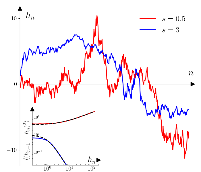
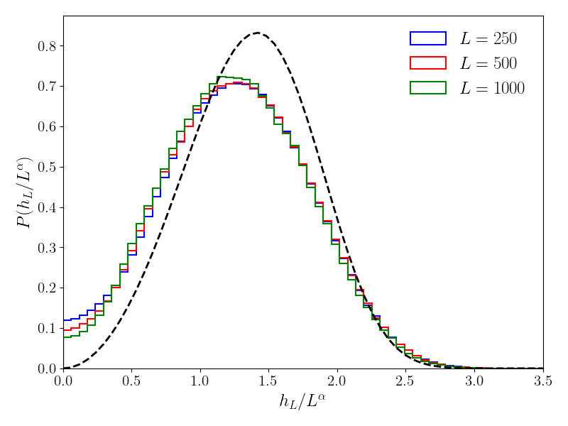
Note that in the above equation, the time dependence of is kept implicit. This equation represents the time evolution of a spring chain characterized by non-homogeneous and -dependent elastic constants . Different behavior of can be considered with the only constraint that . In this paper, we study the power-law case, for large with and even. At the origin, the behavior is regularized with (See SM for the precise form of used in numerical simulation). In Fig.1, we show two interfaces in the stationary regime. The interface with is flatter compared to the case . Indeed, for large , since the springs become stiff when and soft when . One of the main result of this paper is the following prediction for the roughness and dynamical exponents
| (3) |
This prediction verifies the exact exponent relationWolf and Villain (1990)
| (4) |
valid for conservative dynamics with non conserved noise 111Indeed, integrating the SPME equation (1) over the system volume leads to , and thus to the exponent relation.. First, we perform a functional RG calculation and find stable fixed points that preserve the same power law behavior at large . This leads to the prediction Eq. (3) for , obtained to first order in a expansion, but argued to be exact for . However, we also find that local observables exhibit anomalous scaling. For instance, for and , the moments of the stationary equal time height-to-height correlation read:
| (5) |
where indicates the average over the noise. In Eq.(5), is commonly referred to as the local roughness exponent López (1999); Krug (1994); Bernard et al. (2024); Lopez and Schmittbuhl (1998) and can depend on the value of . The anomalous scaling arises due to the presence of inhomogeneous increments, , along the interface.
Third, in the final part of the Letter, we show with heuristic arguments and numerical simulations, that the stationary interface of the SPME, provided that is large, has the same statistical properties as the following random walk:
| (6) |
where is a centered unit Gaussian random variable, independent of . Using this mapping, we can recover the roughness exponent from Eq.(3) as well as the anomalous scaling. In particular, we predict that for while for , one has
| (7) |
with .
Renormalization group. To perform the RG analysis of the SPME (1) we use the Martin-Siggia-Rose dynamical field theory in space dimension , near the upper critical dimension , in a perturbative expansion in . The RG analysis of this model was first performed in Antonov and Vasil’Ev (1995) within a polynomial expansion of the function keeping only first few terms. Here we analyze it in the full functional form, that is necessary to identify all possible fixed points which are determined by the large behavior of . We introduce an infrared renormalization scale (an inverse length scale which can be taken as ). We denote the bare potential in the dynamical action by , where is the bare diffusivity, and the -dependent renormalized potential at scale by , defined from the effective action. The functional RG flow to one loop (i.e. to first order in ) then reads SM
| (8) |
We introduce so that for and in . Let us denote the running at the scale by . The RG equation can be put in the form
| (9) |
which, interestingly, is itself a logarithmic PME. We can look for scale invariant fixed point solutions of the RG flow in the form
| (10) |
Once we find such a fixed point solution, since , one can identify where is the anomalous scaling dimension of . The corresponding time scale is where is the renormalized diffusivity, leading to with . Hence the exact relation follows and there is a single exponent (as the noise is not corrected under RG) see SM for details. Inserting (10) into (9) we obtain the following fixed point equation for with
| (11) |
Since here we consider only the case where is finite at and even, we must have . Moreover, if is solution of (11), so is for any . We therefore choose . We have found through analytical and numerical analysis that there are four types of such solutions to the equation (11):
(i) a line of fixed points with and .
(ii) a special solution associated to .
(iii) associated to .
(iv) solutions diverging at finite as for and for .
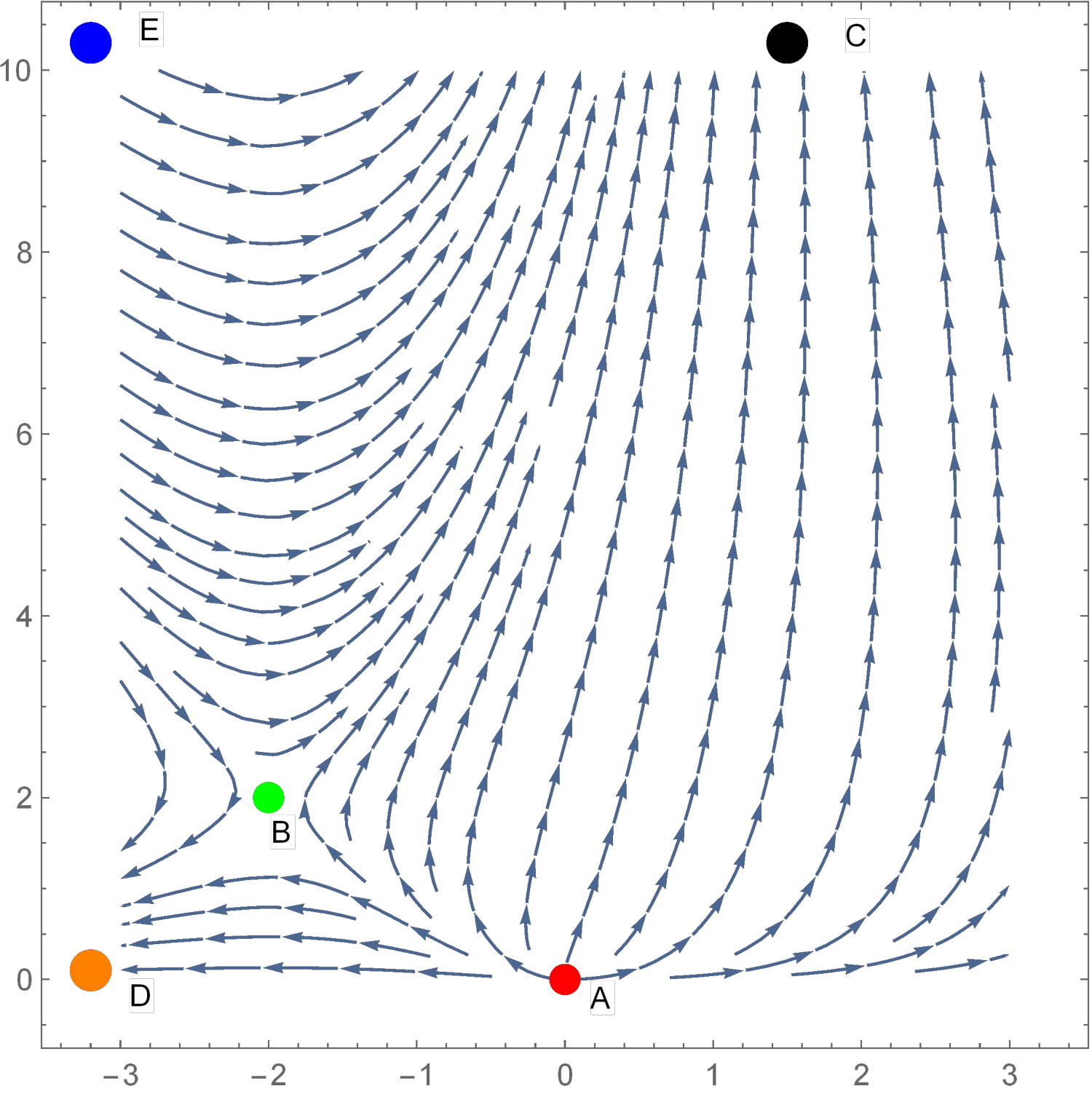
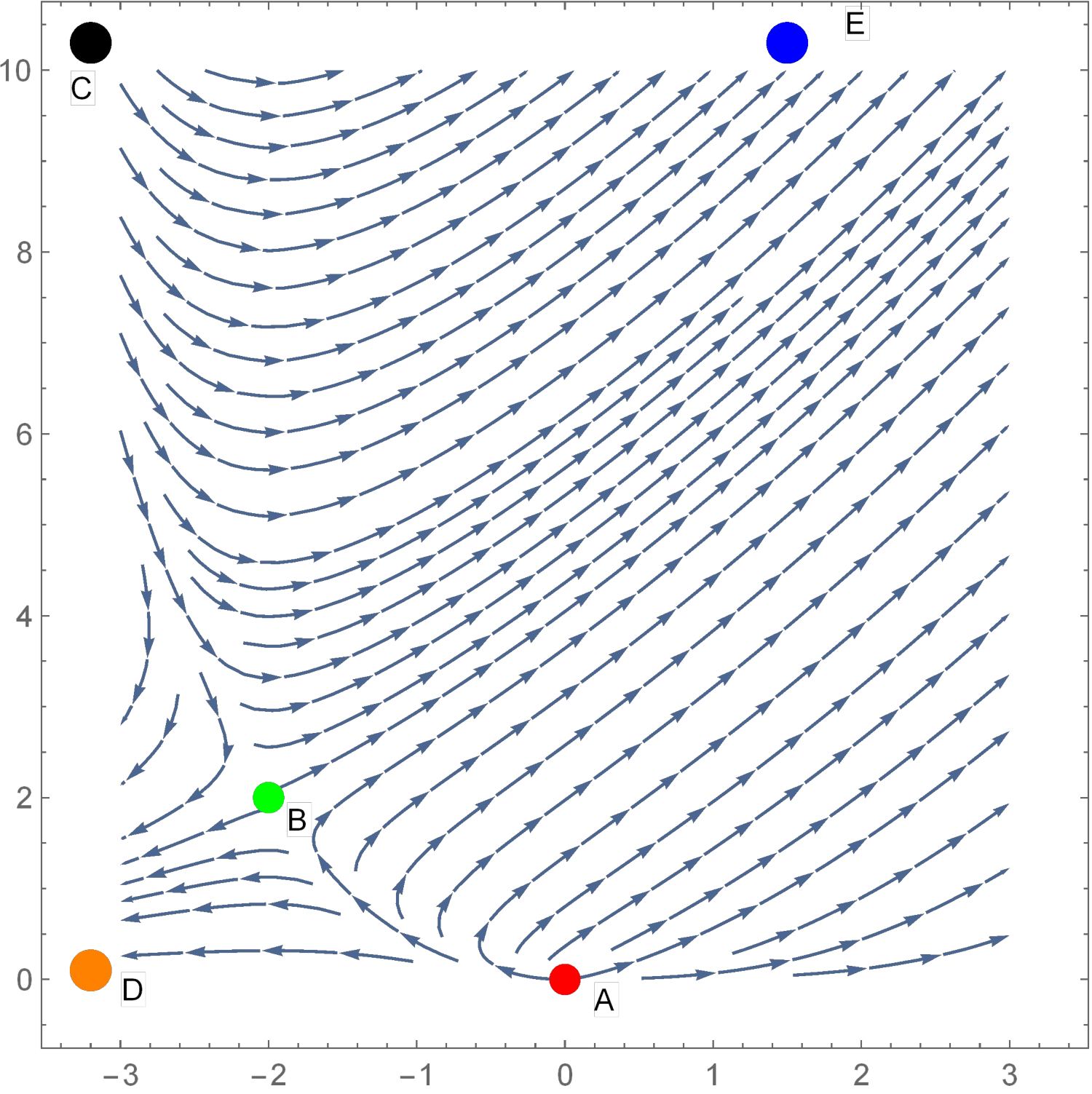
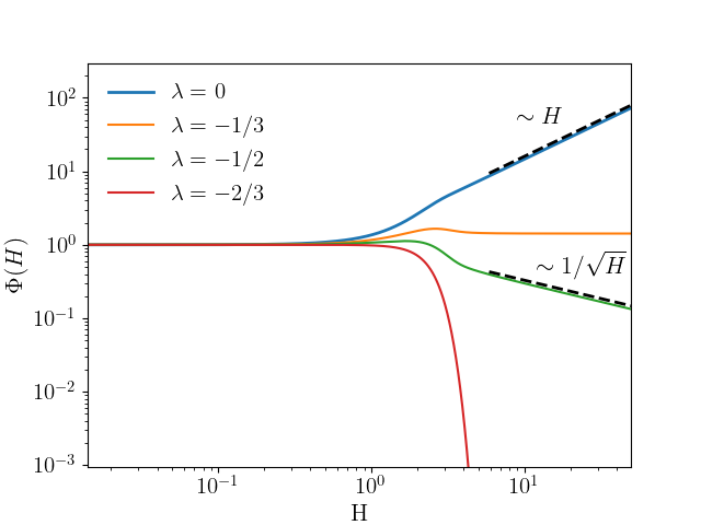
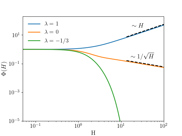
We show by linear stability analysis, see SM , that the solutions (i) which are relevant for this paper correspond to attractive fixed points of the RG flow Eq.(9). In order to study in more details the basin of attraction of these fixed points, we solve Eq.(9) with several initial conditions (See Fig.2). For , the large behavior of is conserved by the RG flow, which converges towards the FP (i) with . Finally, one can argue that the higher order loop corrections to the RG equations (8) and (11) cannot change the large behavior of for , leading to our conjecture that the prediction (3) for the exponents is exact.
Numerical results. We use an Euler scheme to integrate Eq.(2), from a flat initial condition, see SM for details and for our choice of function . We fix and let the right boundary free (). We first compute the time evolution of the width , where denotes the center of mass. Fig.3 shows a very good agreement with Family-Vicsek scaling:
| (12) |
Here the values of the exponents and are the values predicted by the RG (Eq.(3)). The scaling function depends on the boundary conditions, with for and for . Indeed, the interface is rough up to a length , and is flat above this scale. As a consequence, at short times (), the width , as well as the typical height , grow as .
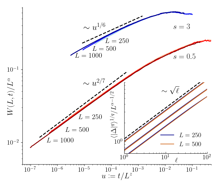
The width is a global observable which probes the behavior of the entire interface. We have also computed local observables, particularly the -th moments of the stationary height-to-height equal-time correlation. In the inset of Fig. 3, we show, for , that it exhibits anomalous scaling behavior for , as displayed in Eq.(5), with the exponent . Here, the average is taken over both the noise but also over . Although Eq.(5) holds for the stationary state, the anomalous scaling can be extended to finite times by replacing by . We will argue that for , while for it depends explicitly on (See Eq.(7)). Finally, we have also studied the structure factor of the height field which also displays the anomalous scaling SM .
Connection to the random walk. To clarify the relation between the random walk (RW) model defined in Eq.(6) and the stationary interfaces of the SPME, we recall that if the spring constants were independent of , i.e. for the EW model, the stationary limit would be described by the equipartition theorem. This theorem predicts Gaussian increments with zero mean and variance . This reasoning can be extended to cases where varies slowly along the -axis, namely . Using a Taylor expansion, we can rewrite the latter condition as a condition for the increments:
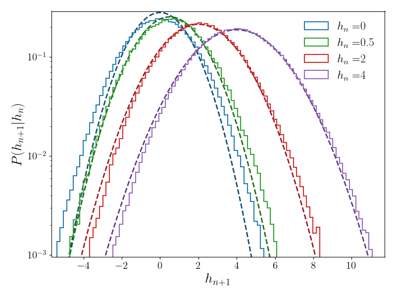
| (13) |
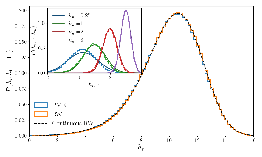
where the asymptotic behavior holds only for large . For small increments, the distribution of conditioned to becomes Gaussian of mean and variance . For large increments, deviations from the Gaussian behavior are observed. However, as can be seen in the inset of Fig.4, these deviations disappear when , in which case the condition (13) is satisfied 222The condition Eq.(13) for the increments can be rewritten as a condition for . Indeed, for small increments, we expect , hence from Eq.(13), the condition becomes . This condition is satisfied for .. This is also confirmed in the inset of Fig.1, where we show that for large . In the stationary regime, for , the height of the interface scale as , hence, in the limit of large system size, we may expect that the statistical properties of the SPME are described by the random walk model of Eq.(6) at all scales. This is indeed what we observe, as detailed in SM and illustrated in Fig. 4.
This RW model allows for several predictions that we now detail. Since the are i.i.d one obtains the second moment of the height difference (removing the tilde symbol)
| (14) |
At large , we assume the scaling , where is the Hurst exponent and is the rescaled height, a random variable independent of . Using we obtain for (see SM for details)
| (15) |
To determine we consider , in which case the r.h.s behaves as while the l.h.s behaves as . Equating the two gives for the RW model, which coincides with the prediction (3) for the SPME in . Furthermore, one can study the local behavior for . From (15) we obtain
| (16) |
which shows that the RW model exhibits anomalous scaling with .
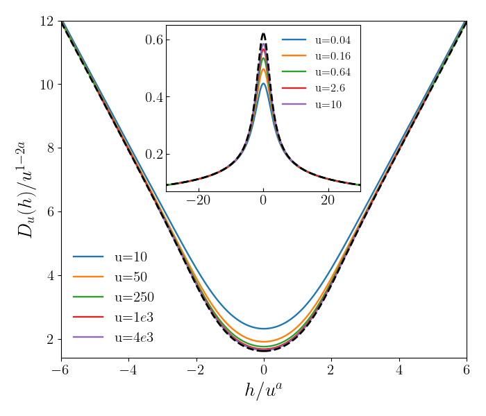
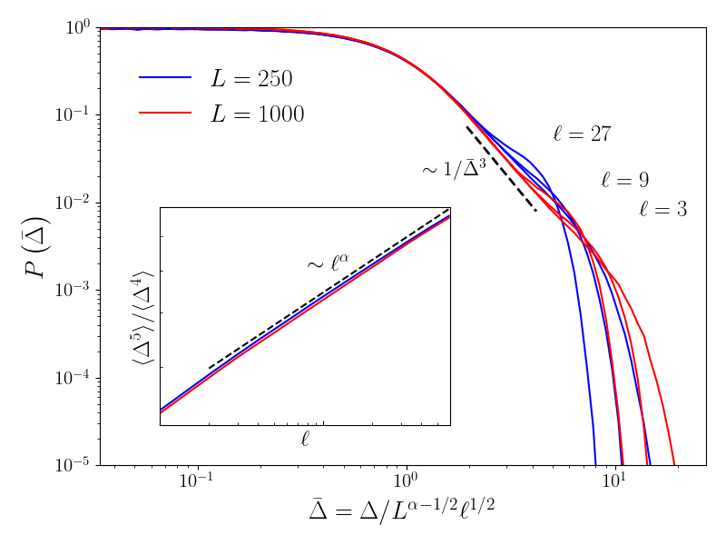
To obtain all the moments of the height difference we need the distribution of the rescaled height at large . This distribution can be obtained using the continuum version of the RW model, analyzed in SM . There we show that this continuum model is related to a Bessel process in the variable . It allows to compute the distribution of the height difference, for given and SM . Its expression depends on the value of . For , it behaves as
| (17) |
with a typical value and an upper cutoff . From (17), we can calculate the -th moment, which shows a multiscaling behavior
| (18) |
with . Indeed, for , the average is dominated by the typical values, namely , while for , it is dominated by the upper cutoff . For , the power law decay of for is replaced by a stretched exponential decay. As a consequence the moments do not display multiscaling and behave as
| (19) |
Averaging over , we obtain for , while, for , we recover the multifractal given in (7). The continuum model enables further predictions, including the determination of the one-point distribution of the rescaled height (see also Fa and Lenzi (2003); giu )
| (20) |
For , this distribution exhibits an integrable divergence at the origin. Conversely, for , the distribution vanishes at the origin and develops a bimodal shape. Furthermore, the two-point height probability, derived in Eq. (S76), is depicted in Fig. 4 and shows excellent agreement with the SPME. This mapping thus provides a detailed characterization of the statistical properties of the stationary interface.
Conclusion. In summary, we have studied the scaling behavior of the stochastic porous medium equation with a diffusion coefficient for , and obtained the critical exponents. We have predicted and verified numerically that it obeys anomalous scaling with non-trivial multiscaling properties for . We have found that the stationary interfaces are remarkably well described by a random walk model, which enables many analytical predictions. Its large scale continuum limit is related to a Bessel process, allowing for calculation of, e.g., the stationary height distribution as well as the multifractal exponents. Using functional RG method we have shown that for arbitrary even functions there exists only four families of fixed points finite at . While only one of them is relevant for the scaling behavior of the SPME, the others could also have applications. In particular, our functional RG equation can be used to study the models of brain dynamics, such as considered in Tiberi et al. (2022).
Acknowledgments: We thank Bjorn Birnir for discussions. AAF acknowledges support from the ANR Grant No. ANR-18-CE40-0033 (DIMERS), AR from the ANR Grant No. ANR-23-CE30-0031-04 and PLD from the ANR Grant ANR-23-CE30-0020-01 (EDIPS). This work was performed using HPC resources from GENCI-IDRIS (Grant 2024-AD011015488).
References
- Vazquez (2006) J. V. Vazquez, The Porous Medium Equation: Mathematical Theory (Oxford Science Publications, 2006).
- Barenblatt (1952) G. Barenblatt, Prikl. Mat. Mekh 16, 67 (1952).
- Zel’dovich and Kompaneets (1950) Y. B. Zel’dovich and A. Kompaneets, Collection of Papers Dedicated to 70th Birthday of Academician AF Ioffe, Izd. Akad. Nauk SSSR, Moscow , 61 (1950).
- Varadhan (1991) S. R. S. Varadhan, Communications in Mathematical Physics 135, 313 (1991).
- Oelschläger (1990) K. Oelschläger, Journal of Differential Equations 88, 294 (1990).
- Gonçalves et al. (2007) P. Gonçalves, C. Landim, and C. Toninelli, Annales De L Institut Henri Poincare-probabilites Et Statistiques 45, 887 (2007).
- Cardoso et al. (2023) P. Cardoso, R. d. Paula, and P. Gonçalves, Nonlinearity 36, 1840 (2023).
- Spohn (1993a) H. Spohn, Journal de Physique I 3, 69 (1993a).
- Spohn (1993b) H. Spohn, Journal of Statistical Physics 71, 1081 (1993b).
- Bántay and Jánosi (1992) P. Bántay and I. M. Jánosi, Physica A: Statistical Mechanics and its Applications 185, 11 (1992).
- Bulchandani et al. (2020) V. B. Bulchandani, C. Karrasch, and J. E. Moore, Proceedings of the National Academy of Sciences 117, 12713 (2020).
- Pedron et al. (2005) I. Pedron, R. Mendes, T. Buratta, L. Malacarne, and E. Lenzi, Physical Review E 72, 031106 (2005).
- Edwards and Wilkinson (1982) S. F. Edwards and D. Wilkinson, Proceedings of the Royal Society of London. A. Mathematical and Physical Sciences 381, 17 (1982).
- Kardar et al. (1986) M. Kardar, G. Parisi, and Y. C. Zhang, Phys. Rev. Lett. 56, 889 (1986).
- Pastor-Satorras and Rothman (1998a) R. Pastor-Satorras and D. H. Rothman, Phys. Rev. Lett. 80, 4349 (1998a).
- Pastor-Satorras and Rothman (1998b) R. Pastor-Satorras and D. H. Rothman, Journal of Statistical Physics 93, 477 (1998b).
- Antonov and Kakin (2017) N. V. Antonov and P. I. Kakin, Theoretical and Mathematical Physics 190, 193 (2017).
- Birnir and Rowlett (2013) B. Birnir and J. Rowlett, International Journal of Nonlinear Sciences and Numerical Simulation 14, 323 (2013).
- Pelletier (1999) J. D. Pelletier, Journal of Geophysical Research: Solid Earth 104, 7359 (1999).
- Hwa and Kardar (1989) T. Hwa and M. Kardar, Physical Review Letters 62, 1813 (1989).
- Tiberi et al. (2022) L. Tiberi, J. Stapmanns, T. Kühn, T. Luu, D. Dahmen, and M. Helias, Physical Review Letters 128, 168301 (2022).
- (22) N. Papanikolaou, T. Speck, Dynamic renormalization of scalar active field theories, arXiv:2404.09999.
- Barbu et al. (2016) V. Barbu, G. Da Prato, and M. Röckner, Stochastic porous media equations, Vol. 2163 (Springer, 2016).
- Da Prato and Röckner (2004) G. Da Prato and M. Röckner, Journal of Evolution Equations 4, 249 (2004).
- Kim (2006) J. U. Kim, Journal of Differential Equations 220, 163 (2006).
- Barbu et al. (2009) V. Barbu, G. D. Prato, and M. Röckner, Communications in Mathematical Physics 285, 901 (2009).
- Dareiotis et al. (2021) K. Dareiotis, M. Gerencsér, and B. Gess, in Annales de l’Institut Henri Poincaré (B) Probabilités et Statistiques, Vol. 57 (Institut Henri Poincaré, 2021) pp. 2354–2371.
- (28) The stochastic PME has been studied numerically in Nagatani (1991). However the result is inconsistent with our results, and may be the consequence of an incorrect discretization procedure.
- López (1999) J. M. López, Phys. Rev. Lett. 83, 4594 (1999).
- Krug (1994) J. Krug, Phys. Rev. Lett. 72, 2907 (1994).
- Bernard et al. (2024) M. Bernard, P. Le Doussal, A. Rosso, and C. Texier, Physical Review E 110, 014104 (2024).
- Lopez and Schmittbuhl (1998) J. M. Lopez and J. Schmittbuhl, Phys. Rev. E 57, 6405 (1998).
- (33) See Supplemental Material.
- Wolf and Villain (1990) D. Wolf and J. Villain, Europhysics Letters 13, 389 (1990).
- Note (1) Indeed, integrating the SPME equation (1\@@italiccorr) over the system volume leads to , and thus to the exponent relation.
- Antonov and Vasil’Ev (1995) N. V. Antonov and A. N. Vasil’Ev, Journal of Experimental and Theoretical Physics 81, 485 (1995).
- Note (2) The condition Eq.(13\@@italiccorr) for the increments can be rewritten as a condition for . Indeed, for small increments, we expect , hence from Eq.(13\@@italiccorr), the condition becomes . This condition is satisfied for .
- Fa and Lenzi (2003) K. S. Fa and E. K. Lenzi, Physical Review E 67, 061105 (2003).
- (39) While this work was in completion, the continuum RW model was studied independently in Del Vecchio and Majumdar (2024).
- Nagatani (1991) T. Nagatani, Physical Review A 43, 5500 (1991).
- Del Vecchio and Majumdar (2024) G. Del Vecchio and S. N. Majumdar, (2024), arXiv:2410.22097 [cond-mat.stat-mech] .
- Wetterich (1993) C. Wetterich, Physics Letters B 301, 90 (1993).
- Morris (1994) T. R. Morris, International Journal of Modern Physics A 9, 2411 (1994).
- Balents and Le Doussal (2005) L. Balents and P. Le Doussal, Annals of Physics 315, 213 (2005).
- Schehr and Le Doussal (2003) G. Schehr and P. Le Doussal, Physical Review E 68, 046101 (2003).
- Le Doussal (2010) P. Le Doussal, Annals of Physics 325, 49 (2010).
- Duclut and Delamotte (2017) C. Duclut and B. Delamotte, Physical Review E 96, 012149 (2017).
- Duclut (2017) C. Duclut, Nonequilibrium critical phenomena : exact Langevin equations, erosion of tilted landscapes., Ph.D. thesis (2017).
- Vázquez (2006) J. L. Vázquez, Smoothing and decay estimates for nonlinear diffusion equations: equations of porous medium type, Vol. 33 (OUP Oxford, 2006).
- Balog et al. (2017) I. Balog, D. Carpentier, and A. A. Fedorenko, (2017), arXiv:2410.22097 [cond-mat.dis-nn] .
- Balog et al. (2018) I. Balog, D. Carpentier, and A. A. Fedorenko, Physical Review Letters 121, 166402 (2018).
- Wikipedia contributors (2024) Wikipedia contributors, “Bessel process,” (2024), accessed: 2024-11-07.
- Le Doussal and Wiese (2009) P. Le Doussal and K. J. Wiese, Physical Review E—Statistical, Nonlinear, and Soft Matter Physics 79, 051105 (2009).
.
The stochastic porous medium equation in one dimension
– Supplemental Material –
Maximilien Bernard,1,2 Andrei A. Fedorenko,3 Pierre Le Doussal,1 and Alberto Rosso2
1Laboratoire de Physique de l’Ecole Normale Supérieure,
CNRS, ENS and PSL Université, Sorbonne Université,
Université Paris Cité, 24 rue Lhomond, 75005 Paris, France
2LPTMS, CNRS, Univ. Paris-Sud, Université Paris-Saclay, 91405 Orsay, France
3Univ Lyon, ENS de Lyon, CNRS, Laboratoire de Physique, F-69342 Lyon, France
In this Supplemental Material, we give the principal details of the calculations described in the main text of the Letter.
I Functional RG approach
I.1 Dynamical action and field theory
We study the isotropic SPME equation in space dimension
| (S1) |
where is a Gaussian white noise with zero mean and variance
| (S2) |
Here we use the subscript zero to denote the bare quantities. We use the dynamical action, obtained by enforcing the equation of motion using an auxiliary response field , and averaging over the noise. As a result the average of any observable of the solution of (S1) over the noise can be written as a path integral
| (S3) |
where the dynamical action reads
| (S4) |
and one may include the initial conditions in the definition of the path integral if needed. An infrared cutoff is implicit everywhere to regularize the system at large distance (alternatively one may use a finite system size ). Splitting , where is the bare diffusivity and can be treated as the non-linear interaction, one sees from the quadratic part of the action that the bare dimensions of the fields are and , with scaling with , and that the non-linear part becomes relevant for . One thus expects logarithmic divergences in perturbation theory at the upper critical dimension . Since the field is dimensionless there one expects the need for functional RG to describe the flow of the full function .
One proceeds by computing the effective action functional associated to the action , using the two component field notation whenever convenient. Let us recall that one first defines the partition sum in presence of sources, . Then is the generating function of the connected correlations of the field (obtained by taking successive derivatives w.r.t ). is then defined as the Legendre transform of , i.e. . Its important property is that connected correlations of are now tree diagrams obtained from . Hence the vertices of are the dressed (or renormalized) vertices which sum up all loops. Decomposing where is the part of the action which is quadratic in the fields, it can be computed from the perturbative formula
| (S5) |
where denote an average over the field (at fixed background field ) keeping only 1-particle irreducible diagrams (i.e. connected diagrams in the vertices which cannot be disconnected by cutting a propagator from ). The RG analysis then proceeds by considering the leading dependence of in the IR cutoff as , which is related to the analysis of the divergences in the 1PI diagrams (loop diagrams).
I.2 Effective action and RG flow
The calculation of associated with the action (S4), the analysis of the divergences, and the ensuing RG analysis was pioneered in Antonov and Vasil’Ev (1995). Here, we thus only sketch the main ideas, and refer the interested reader to that paper for details, as well as to the subsequent paper Antonov and Kakin (2017), which discusses an anisotropic version of the model studied in the context of erosion.
There it was found that to one loop it takes the same form as the action (S4)
| (S6) |
up to terms which are irrelevant near (higher gradients). Indeed, one can check that the term is not corrected, and that, furthermore, the term is also not corrected, so that (and we choose below). It is easy to see since a shift by a uniform constant in (S4) produces only quadratic terms, up to boundary terms. Equivalently, the term can be integrated by part into hence no correction to the uniform part of can be produced. As a consequence, no wave-function renormalization, i.e. no renormalization of the field , is needed and the only quantity which flows is , the -dependent renormalized potential.
In Antonov and Vasil’Ev (1995) it was shown that the divergent part of the one loop contribution to the effective action reads, near , with
| (S7) |
where is the IR regulator (renormalization mass) and . Note that in Antonov and Vasil’Ev (1995) the one loop correction (S7) was used to study the RG flow only for the first few coefficients in the Taylor expansion of , see below. However, in order to identify all possible fixed points, it is necessary to consider the full functional flow of , which is done in this work. To that end we compute the one-loop correction to the full potential expressed in terms of the functional diagram
| (S8) |
corresponding to the lowest order correction in (S5). Here the black square stands for the vertex and the solid line for the correlation function of in the presence of the background field ,
| (S9) |
where we include the IR cutoff . Evaluating the integrals and expanding in we arrive at
| (S10) |
Taking a derivative w.r.t. at fixed , and then replacing , we obtain the RG flow for the full potential to leading order in as
| (S11) |
This equation can alternatively be obtained from the exact RG functional equation for .
The general exact RG method was developed in Wetterich (1993); Morris (1994) and
leads to an exact RG equation for the functional (see also Section 3 in Balents and Le Doussal (2005)
for a simplified summary).
To arrive at (S11) requires
truncations, which can be performed in a systematic way in a multilocal expansion Schehr and Le Doussal (2003); Le Doussal (2010),
and within a controlled dimensional expansion near . These truncations can be performed more
generally within the non-perturbative FRG approach, which was applied to the anisotropic version of the model (erosion)
in
Duclut and Delamotte (2017); Duclut (2017). Here we consider perturbative FRG applied to the isotropic model.
Comparison with the RG flow of Antonov and Vasil’Ev (1995). Let us now compare our functional RG flow (S11) to the one displayed in Antonov and Vasil’Ev (1995). To this aim we define a scaled potential via
| (S12) |
where the are the dimensionless couplings defined in Antonov and Vasil’Ev (1995). Note that implicitly depend on . By definition one has and . Taking derivatives at of the RG flow equation (S11), and using (S12), we first obtain the flow of the diffusivity as
| (S13) |
which coincides (23a) in Antonov and Vasil’Ev (1995). Using (S13) and (S12), taking into account that also depends on via (S13) we obtain
| (S14) | |||
| (S15) |
which is in agreement with (23b) in Antonov and Vasil’Ev (1995) (their functions have by definition the opposite sign and there is an obvious sign misprint in the first term of their ).
It was argued in Antonov and Vasil’Ev (1995) that the infinite-dimensional space of the couplings has a two dimensional surface of fixed points parameterized by the values of and , and the conclusion was that studying the nature of these fixed points is a difficult task. The authors of Antonov and Vasil’Ev (1995) summarize: ”The general conclusion is pessimistic: the problem of building a satisfactory microtheory of the given phenomenon remains unresolved.” In fact this problem can not be resolved once one truncates the as done in Antonov and Vasil’Ev (1995). Indeed, as we show below, the fixed point is selected by the large behavior of the bare and to identify it one needs to consider the full functional flow.
I.3 Critical exponents
The critical exponents are associated to scale invariant solutions of the RG flow. Let us first examine the form that these solutions can take. To analyze (S11) let us replace the variable by the variable
| (S16) |
where is the bare IR cutoff, and we are interested in the limit . In that limit we see that for , and in . As we pointed out in the main text, the running derivative of the potential, which we denote (indicating the explicit dependence) satisfies (taking in (S11)) a logarithmic PME
| (S17) |
As we will discuss in Sec. II this equation admits the so-called self-similar solutions of the form
| (S18) |
where is a fixed function with finite, and the exponent takes some given value (depending on , see below). Since the self-similar solutions of the form (S18) lead to scale-invariant behavior and can act as attractors in the large limit, they can be referred to as fixed points of the RG flow.
Recalling that where is the IR cutoff, we have where is the system size. The form of the fixed point solution (S18) implies the scaling behavior
| (S19) |
Let us recall that the bare two point height correlator reads in Fourier, from the second derivative in (S4) (or equivalently from (S1))
| (S20) |
The exact (renormalized) correlator is similarly obtained from the second derivative matrix and takes the scaling form (setting ) for small
| (S21) |
where as follows from (S18)
| (S22) |
This implies that the dynamical exponent defined by is
| (S23) |
and obeys the general relation given in the text. Furthermore from (S21) we see that in real space the equal time correlation
| (S24) |
consistent with the prediction for the roughness exponent given by (S19).
II Functional RG flow: fixed points and their stability
The RG flow equation (S17),
| (S25) |
is itself a logarithmic fast diffusion equation, which represents a limiting case () of the fast diffusion equations, i.e. PMEs with , see Chap 8. in Vázquez (2006) for details and applications. The solutions of these non-linear diffusion equations are expected to asymptotically approach, for large , a self-similar solution, independently of the initial condition . In the RG picture this self-similar solution corresponds to a fixed point. We consider the forward or type I self-similar solutions of the form (S18),
| (S26) |
with independent of for large , which we denote . The RG flow for reads
| (S27) |
where primes mean the derivative w.r.t. . A self-similar solution is given by function which satisfies Eq. (11),
| (S28) |
Note that if is a solution of this equation, then is also a solution for any .
For the problem studied in this paper we will eventually restrict to solutions where is finite and positive for all and even in . However we will first study the most general solutions of (S28).
II.1 Classification of fixed points: Phase-plane formalism
In order to classify all possible self-similar solutions and identify their properties, we can apply the phase-plane formalism see e.g. Section 3.8.2. in Vázquez (2006). To that end, we rewrite equation (S28) for as an autonomous system of two first-order differential equations for the functions and , which does not explicitly depend on ,
| (S29) | |||||
| (S30) |
where and so on. Each solution to the system (S29)-(S30) corresponding to a self-similar solution can be represented by an integral curve in the phase plane . Only one integral curve passes through each point in the phase plane. The system (S29)-(S30) has several singular points in the phase plane and each solution corresponds to an integral curve connecting two of them. Expansion around singular points provides us the asymptotic behavior of for (in the case of starting point) and (in the case of ending point). Thus the analysis of the singular points of the system gives exhaustive list of all fixed points with their asymptotic behavior for large and small .
One can rewrite the system (S29)-(S30) as a single differential equation,
| (S31) |
We consider the fixed points with , and thus, we look only at the integral curves in the upper plane . The integral curves connecting different singular points in the phase plane for and are shown in Fig. 5. The system has two finite singular points in the plane : and whose position does not depend on , and three points at infinity: , , .
We now study the asymptotic behavior at each of these singular points, and identify among them repeller and sink points which can be only starting or ending points for the integral curves.
(A) Expanding the system of equations (S29)-(S30) around point A we obtain
| (S32) | |||||
| (S33) |
Diagonalizing it, we find the eigenvalues . Thus the point A is a repeller and the integral curves can only start at it. Equation (S33) implies for small , where is a constant. This leads to at for all solutions which start at point A.
(B) Expanding around point B: and we obtain to linear order
| (S34) | |||||
| (S35) |
Computing the eigenvalues we find for all . Thus the point B is a saddle point: there are integral curves starting and ending at the point B. Close to B the solution behaves as for small if it is a starting point and for large is it an ending point.
(C) Close to the singular point C the solution has the form
| (S36) | |||||
| (S37) |
This point is a sink point for with the asymptotic behavior for large , and a repeller point for with for small . In the latter case the solution diverges at the origin since for .
(D) Close to the point D the system can be simplified to
| (S38) | |||||
| (S39) |
This point is a sink. The solution in its vicinity is given by and with constants . The corresponding solutions have the asymptotic behavior of the form for large .
(E) Close to the point E the system can be simplified to
| (S40) | |||||
| (S41) |
whose solution, and , diverges at finite . The singular point E is a sink for and a repeller for . Thus, for the corresponding self-similar solution is defined for with and diverges in the limit , while for it is defined for and diverges in the limit . The above form of and implies the asymptotic behavior slightly below for and above for . Expanding it in a Laurent series near the pole , we obtain . The coefficient in the leading term is exact, as we checked numerically at fixed .
For the system (S29)-(S30) simplifies to
| (S42) | |||||
| (S43) |
whose solution is and
. This leads to an exact self-similar solution . This solution is negative for and decays as for large . For it diverges at finite , as .
We are now in the position to analyze all possible self-similar solutions. Here we restrict ourselves to the solutions which are finite in the vicinity of the origin . Only the solutions represented by the integral curves starting at point satisfy this condition. There are four different classes of such solutions corresponding to the integral curves connecting the point A with points B,C, D or E:
() This solution decays as for large .
() This solution exists only for and behaves as for large .
() This solution decays as for large .
() This solution exists only for and diverges at finite .
Let us give here some additional properties, as well as a few exact solutions which can be obtained for some values of
For there is a special solution
| (S44) |
which is a limiting case of a more general family of solutions for
| (S45) |
which however are not even in , except in the limit where one recovers (S44).
For there is a solution of the form
| (S46) |
which is even but diverges at . As discussed above, there are additional solutions, which however are not even or not positive.
Remark. For the fixed point behaves at large as with . One can check that it takes the form , where the function satisfies a closed differential equation. Solving in an expansion at large , one finds with , , and so on (up to the rescaling ). Most notably we find the leading correction is always , with a universal coefficient (i.e independent of ). This remark helps to understand the structure of the flow towards the fixed point, see below.
II.2 Numerical calculation of fixed points
We now study numerically the solutions of (S28). Since the flow (S25) preserves the parity of , and the initial conditions considered in this paper are even functions, it follows that we should focus on even, positive, with finite and . Moreover, if is a solution to Eq. (S28), then is also a solution. Hence, we can impose the condition . To perform numerical integration, we first transform equation (S28) into a system of two first-order differential equations for and :
| (S47) | |||
| (S48) |
Starting from the chosen initial conditions, and , we employ a fifth-order Runge-Kutta integration scheme to solve the system numerically.
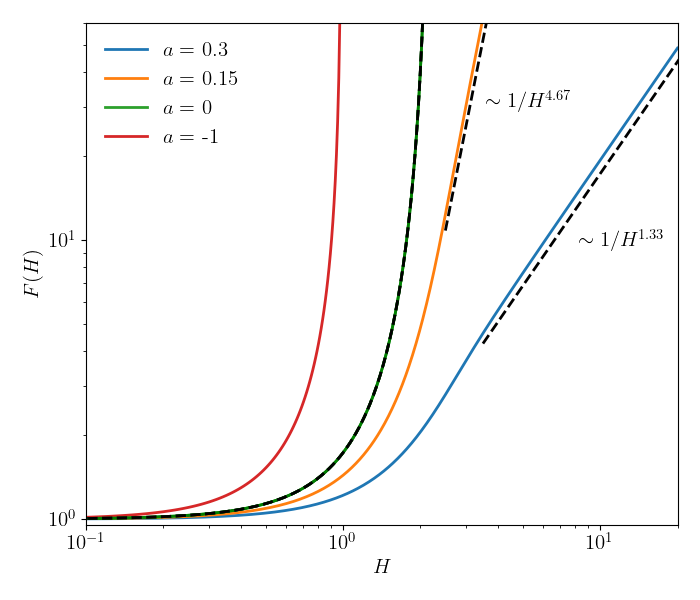
According to the classification of possible fixed points performed in Sec. II.1 we expect four different types of solutions. In Fig. 6 Left, we recover two of them:
-
•
the class (). For , diverges at finite , and for , we recover the exact solution .
-
•
the class (). Shown here for , the solutions exhibit an asymptotic behavior .
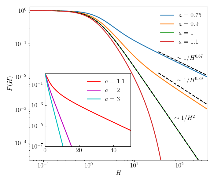
In Fig. 6 Right, we recover the remaining cases:
-
•
the class (). Shown here for when decreases with
-
•
the class (). For , we recover the exact solution .
-
•
the class (). For , we find solutions that decay exponentially.
Note that the behavior of changes qualitatively at and .
II.3 Linear stability analysis
Finding the fixed points alone is insufficient, as they may not be relevant. Therefore, we analyze their stability to determine whether the fixed points are attractive. Here will restrict the analysis to the power law case () , although some of the equations below are more general. We examine the linear stability of the fixed point using the flow equation (S25). To achieve this, we linearize the equation (S25) around the fixed point by introducing a perturbation , defined as:
| (S49) |
where is the eigenvalue that we aim to estimate. We must restrict to perturbations which are smaller or at most of order at large . Indeed, if it is not the case these will flow to another fixed point characterized by a smaller value of . The fixed point will be stable if no such perturbation exist with a strictly positive eigenvalue. By substituting (S49) into the flow equation (S25) and expanding to linear order in , we derive the following linear differential equation for :
| (S50) |
Equivalently, the flow of a perturbation of the fixed point is given by and we want to find the spectrum of , i.e. its eigenvalues and associated eigenvectors , such that .
We have studied the equation (S50) analytically and numerically. From parity one must choose , and since it is a linear equation we can choose . For the numerical integration, we simultaneously solve for and by converting the two second-order equations into a system of four first-order equations for , , , and . As previously done for , we use a Runge-Kutta integration scheme. The only parameter is .
We have found the following results:
- •
-
•
The second symmetry is , which gives the exact eigenvalue corresponding to the eigenvector . It behaves at large as .
-
•
There is a continuum spectrum with eigenvectors which behave as power laws with eigenvalue and . This value of can be simply verified by injecting the large behavior in (S50). The existence of these eigenvectors is easily checked numerically.
-
•
In addition to the continuum spectrum there is a discrete spectrum which correspond to eigenvectors with fast decay at large (stretched exponential). The most relevant one has eigenvalue . It can be found exactly as follows. Consider the change of function
(S51) Then (S50) is equivalent to the Schrodinger problem
(S52) (S53) Hence must be a zero energy eigenvector of the Schrodinger problem in the potential . For the case , we see that has the familiar form which arises in supersymmetric quantum mechanics, and an eigenvector is then
(S54) which has a fast decay at infinity. Hence we have found an exact eigenfunction , associated to the eigenvalue , of our original problem. Interestingly it behaves at large as , reminiscent of the behavior of in (S66) (although we could not see any obvious relation). Next, since one can write with , we see that no fast decaying eigenvector can exist for since then must have a positive spectrum. Finally note that in the variable the linearized flow equation reads .
We have confirmed the above result by computing numerically the eigenvector for , and we have other fast decaying eigenvector for a set of discrete values of , which are all smaller than . In order to identify these eigenvalues numerically, we note that is a smooth function of as the differential equation is linear. Therefore, when , we have , where is a smooth function of . Therefore, to find a function with exponential decay, must hold. One can then assume that changes sign near this root.
Finally, we have shown that, for , eigenvectors are associated to negative eigenvalues, provided they decay faster than at large . Hence these fixed points are stable.
II.4 Basin of attraction
We previously showed that the fixed points found of the form are stable for . A more precise test consists in starting from the initial conditions and checking that the RG flow indeed converges towards the self-similar solutions obtained earlier. To evaluate numerically the flow equation
| (S55) |
we consider a large finite grid of spacing : . We evaluate the discrete Laplacian using . At the boundaries, we take the Laplacian to be equal to the one evaluated in respectively and . We then integrate with respect to using a Euler scheme with an integration step .
We focus on the case . In particular, in the main text, we considered and . For , we take the initial condition , which is analytic in , and . For , we consider and . For large , since one has , it is necessary to use a smaller integration step . In Fig. 2 of the main text, we show that, in both cases, under the RG flow equation (S55) the asymptotic behavior at large is preserved, and that converges towards the self-similar fixed point with the asymptotic behavior (), and the corresponding parameter . This confirms that the fixed points studied previously are stable, and more importantly, that they attract the functions of the form chosen in this paper.
Thanks to linear stability analysis, we can elucidate the approach to the fixed point, by determining the largest eigenvalue and the form of its corresponding eigenvector . Apart from a discrete set of eigenvectors that decay exponentially fast, with the largest eigenvalue being , all other eigenvectors exhibit power-law decays. There are potentially two relevant power-law eigenvectors.
-
•
Starting from initial conditions of the form , the second term will be corrected during the flow and decay with eigenvalue (given that ).
-
•
Recall that the fixed point takes the form . The second power law will arise during the flow and is associated to the eigenvalue .
Therefore, the largest eigenvalue is either , or . However, the latter is always irrelevant since . Ultimately, we find that the largest eigenvalue and the form of its corresponding eigenvector depend on the values of and . For , , and the largest eigenvalue is , leading to decaying as a power-law. For , the largest eigenvalue is , and the leading eigenvector decays exponentially fast in . This is illustrated in Fig. 8. On the left, starting from initial conditions , corresponding to and , we expect the largest correction of to scale as . The eigenvector is given by (S54), up to a constant, chosen to match the behavior at . indeed decays exponentially in , although there is a slight difference with the analytical solution, likely caused by the finite . On the right panel, the initial condition is , corresponding to and . In this case, , and the largest eigenvalue is . Its corresponding eigenvector behaves as in the limit . Both these properties are checked numerically in Fig. 8.
III Predictions from the random walk model
The random walk model allows for very detailed predictions. We will study the discrete random walk model but at large scale one can use a continuum description which we will also study.
III.1 Second moment, scaling and anomalous scaling
We consider the random walk model
| (S56) |
for , where the are i.i.d Gaussian random variables with unit variance. The trajectory of the walker can be identified with an interface in the stationary regime, and its position corresponds to the height of the interface. We recall that at large one has . The increments being independent the variance of the height differences is equal to
| (S57) |
This relation is exact for any . We now consider a random walk with an initial position . At large , we assume the scaling relation , where is the Hurst exponent and is the rescaled height, a random variable that is independent of . The one point distribution of is discussed in Section III.2. Now we determine the exponent using a self-consistent argument. Using (S57) one obtains
| (S58) |
For and for large , we can estimate the r.h.s as
| (S59) |
while the l.h.s. behaves as . Equating both determines and gives a relation between the moments of
| (S60) |
Note that the exponent of the random walk model coincides with our result for the global roughness exponent for the interface, given in the text. Furthermore, we now demonstrate that the random walk exhibits anomalous scaling behavior, as observed numerically for the stationary interface in Figure 3 of the main text. Let us evaluate the variance of the height difference using (S57). In the right hand side we can write for and any
| (S61) |
where is the Hurwitz zeta function. There are two regimes.
In the first regime , which is relevant for the study of local properties, one can neglect the dependence in in the sum in (S61) and one finds an anomalous scaling:
| (S62) |
This corresponds, for all , to a local roughness exponent for the random walk:
| (S63) |
In the second regime, , one recovers the global scaling, more precisely
| (S64) |
We observe that the two regimes match when .
III.2 Distribution of the increments and multiscaling
In order to obtain the local roughness exponents for any and the multiscaling properties of the random walk, one must study the distribution of the increments. To this aim we more information about the distribution of the scaled height . At large it becomes well described by a continuum model for a height field which obeys the Ito stochastic equation where is a Brownian motion. The one point PDF of , satisfies the Fokker-Planck equation
| (S65) |
This equation and the stochastic process are studied in Section, where we show that at large , using with initial condition , the PDF takes the scaling form
| (S66) | |||
| (S67) |
which is normalized as while . One can check explicitly that the moment relation in (S60) holds exactly for this scaled variable . Hence we can identify this variable in the discrete and the continuum model.
Distribution of the local increment
We start by computing the distribution of the increment of length in the discrete model for large . In this case, the discrete setting is particularly convenient as this increment is exactly Gaussian for a given , hence its distribution is given by
| (S68) |
where we use the continuum formula (S66) for the PDF of with . Depending of the value of the region in which dominate the integral are different. Let us consider first the case where the integral is dominated by values of so that we can replace . Inserting (S66) we obtain
| (S69) |
Upon rescaling one obtains
| (S70) | |||
| (S71) |
For and in the large limit, the integral is dominated by small and one can neglect the second term in the exponential. One finds that the function has a power law tail
| (S72) |
where we used . This power law tail is valid for , and the tail exponent diverges as . In summary we thus obtain for
| (S73) |
Note that the power law extends up to an upper cutoff of the order , which is determined by (assuming here that is an increasing function of ).
For , is a decreasing function of , and one can evaluate S71 using a saddle point method. Upon the change of variable one can rewrite
| (S74) |
The function has a single minimum at , and one obtains at large the saddle point estimate
| (S75) |
Hence for the decay is a stretched exponential with an exponent .
While the distribution of the increments of length 1 provides insights into the behavior of the random walk, it is necessary to also compute the distribution of the increments of arbitrary small length to obtain the multiscaling properties, to which we now turn.
Distribution of the height differences
To compute the distribution of the height differences and their moments we will again resort to the continuum model defined above, which becomes exact for large . The correspondence is and . In section LABEL: we derive the propagator of the continuum process with , which is simple when considering the absolute value . Its expression reads
| (S76) |
which is the probability that the absolute value of the height is at , given that it is at . It is normalized to unity when integrating from to . One can check that has a limit when which coincides exactly with the one-point PDF of given in (S66).
This setting is convenient to compute the probability of the increment of the absolute value of the height, , which we do below. We consider the regime , in which case, as we argue below, and typically share the same sign, such that the increments of and of have similar distributions. Using the Markov property of the process, and choosing the initial condition , we can write
| (S77) |
We recall the asymptotics, for , and for .
The contribution of the integral for takes the form
| (S78) |
Consider now , one can expand in and this contribution becomes
| (S79) |
which, for and is exactly the result in (S69), obtained for the discrete model. We verify below that this indeed represents the relevant contribution for . This result indicates that for with , the function typically maintains the same sign. Consequently, the distribution of the increments of and of are similar. Hence, for , the scaling function is given by
| (S80) |
where the function has been calculated in the previous section, see Eq. (S71).
To obtain the behavior for large , we need to examine the contribution from small to the integral in (LABEL:eq:expprobdiff). We focus first on for clarity. Since in that regime one has one can expand the argument of the exponential in small which gives an upper cutoff on of order . This implies that the argument of the Bessel function is small, and we can use the asymptotic form for . Recalling that we consider here , we obtain the contribution
| (S81) |
First note that for , this term is indeed negligible compared to (S80), Indeed, it is of order , which is precisely the same order as is reached in (S80) far in the tail for as can be checked using the asymptotics (S72) of the scaling function . This justifies a posteriori the above claim that the integral in (LABEL:eq:expprobdiff) is dominated by when .
Returning to the case , we see that in the region of integration, , we can expand to first order in . By making the change of variable , we obtain
| (S82) |
where we have used that which holds since we consider the case , . Note that, whether we consider the region of integration or , there is an exponential cutoff at . Therefore, the first region is the relevant one.
In summary we find that the PDF of the increments, , takes schematically the form, for and
| (S83) |
with a stretched exponential decay given by (S82) for larger than the cutoff . Note that in the case , we can see from Eq.(LABEL:eq:expprobdiff) that making the change of variable leads to the same equation as for , except that the last term is replaced by . However, as we assumed , the dependence in in this term turns out to be irrelevant in all the regimes that we considered. This is presumably a signature that for there are essentially no sign changes of .
For there is no power law behavior for the increment distribution and one finds instead a stretched exponential form
| (S84) |
where the stretched exponential constant is given by .
Moments of the height differences
We can now compute the moments of order of the height increments, , from its distribution in the case . For , there are two regimes in .
In the first regime, for , one can use (S80) which leads to
| (S85) |
where is a -dependent amplitude equal to the -th moment of the scaled distribution given in (S80) and (S71). We recall that . Since this distribution has a power law tail , see (S72), this can only hold for , as diverges as .
For the moment is instead dominated by the cutoff of the distribution of , which has a fast stretched exponential decay, see (S82) which leads to
| (S86) |
For , note that, using (S80), one retrieves exactly (S62) obtained in the discrete setting. Recalling that the local roughness exponent is defined by , one thus finds for
| (S87) |
For , one has and thus retrieving the standard EW scaling.
IV Solution of the continuum random walk model
The continuum model is defined by the Ito stochastic equation for
| (S89) |
where is a positive even function of with finite.
IV.1 Mapping to a Langevin equation
One can transform this equation into one with additive noise. We introduce the function . We consider the process . Then using Ito rule, we obtain that it obeys the stochastic equation
| (S90) |
Inverting as , the process satisfies now the following Langevin equation with additive noise and with a drift
| (S91) |
which describes thermal motion (at temperature ) in the potential .
Equivalently, one can perform the same transformation on the Fokker Planck equation. The PDF of satisfies (S65). Defining the PDF of as , one obtains the relation . Inserting in (S65) and using , one obtains the Fokker Planck equation for
| (S92) |
where is given in (S91). This is indeed the FP associated to the process (S91).
Note that it admits formally a zero current equilibrium Gibbs measure , i.e. , which however is normalizable only if decays faster than , i.e. ., which is not the regime considered here.
IV.2 Power law and mapping to a Bessel process
Let us now specialize to the power law case . In that case one has
| (S93) |
The potential is then . It is thus repulsive for and attractive towards for . In both cases however for , undergoes unbounded diffusion in the potential , and obeys the stochastic equation
| (S94) |
Thus one finds that up to its sign, is a Bessel process. More precisely
| (S95) |
Here is a Bessel process Wikipedia contributors (2024), which is defined as the Euclidean norm of the dimensional Brownian motion . One has
| (S96) |
where is the -dimensional BM. Thus one finds that is recurrent for any , since and crosses infinitely often the origin.
To use the properties of the Bessel process we will study . The propagator of the Bessel process, , is known and reads for (i.e. for )
| (S97) |
where is the modified Bessel function. One can check that the current near
| (S98) |
vanishes for , which corresponds to reflecting boundary conditions.
Finally, using that , we readily obtain the propagator in the variable, which is given in (S76).
Remark. Note that the above continuum model (S89) was studied previously
in Fa and Lenzi (2003), where the one-point distribution was obtained, as well
as very recently in Del Vecchio and Majumdar (2024),
although by different methods, and focusing on different observables, such as first passage and occupation times.
Remark The present model is also related to the ABBM model of avalanches, see e.g. Eq (213) in Le Doussal and Wiese (2009). The identification is thus and
| (S99) |
Our present RW model corresponds to the limit . The avalanche exponent (231) for the ABBM model is
| (S100) |
Here it describes the distribution of the where the process returns to zero (up to some small cutoff, see discussion in (232) there).
V Numerical results
V.1 Numerical details
We use an Euler integration scheme to integrate Eq.(2), namely
| (S101) |
where is a Gaussian random variable with unit variance, and is the integration step. To ensure numerical stability, the integration step should be small compared to . This requires a small when , large. Knowing that and , we therefore take for
| (S102) |
For , we set .
One possible choice for is
| (S103) |
with . This choice preserves the parity of and regularizes its behavior at the origin with . While is non-analytic at , this poses no numerical issues. In particular, we verified that it satisfies the scaling relations from the RG.
In order to reach a stationary state, we must consider a situation where the center of mass of the interface remains confined. This is not the case under periodic boundary conditions, as the center of mass undergoes diffusion. Instead, we consider the case where one extremity of the interface is fixed (i.e., ) while the other extremity, , is free (i.e., ). In this setup, the center of mass of the interface will scale as at large times.
V.2 Numerical evidence for the correspondence between stationary interface and the random walk model
In the following, we study the correspondence between a stationary interface, with the right boundary fixed at and the left boundary free, and the random walk model defined by:
| (S104) |
As mentioned in the main text, we expect this correspondence to hold when the interface varies slowly, i.e.
| (S105) |
When this condition is met, and, considering the chosen form (S103) of , this leads to the condition:
| (S106) |
This condition is always satisfied for sufficiently large values of . However, it can also hold for small if is large enough for , or small enough for .
In Fig. 9 (Left), we test the validity of the condition (S105). For small increments, the distribution of conditioned to becomes Gaussian of mean and variance . For large increments, deviations from the Gaussian behavior are observed. However, these deviations disappear when , in which case the condition (S105) is satisfied. Numerically, the distribution of is obtained by considering a small window around . In practice, we take for ; for ; for ; for .
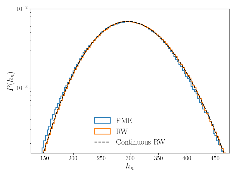
In Fig. 9 (Right), we show the distribution of (with ) for an interface with the left boundary fixed at for . We choose and sufficiently small such that . Under these conditions, we expect the SPME interfaces to be well-described by the random walk model. The prediction from the continuous RW (S76)) is for the process , but which is equivalent to the process here as remains positive. The random walk model provides a good approximation, although some discrepancies appear for smaller values of .
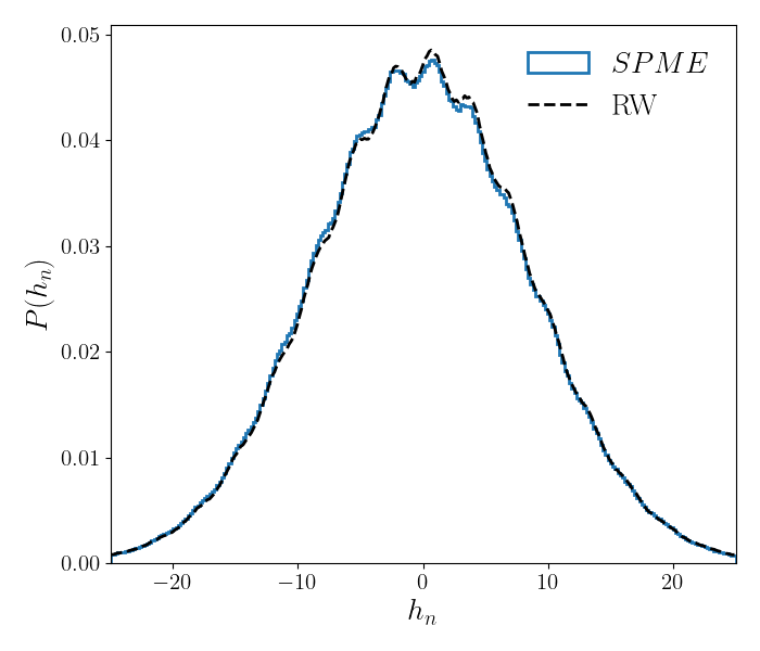
The SPME/RW mapping is expected to be satisfied for any function that varies slowly, i.e., satisfies the condition (S105). As an example, in Fig. 10, we show the distribution of for an interface starting from and with , and observe a good agreement with the random walk obtained numerically. We use the discretization of the Laplacian with .
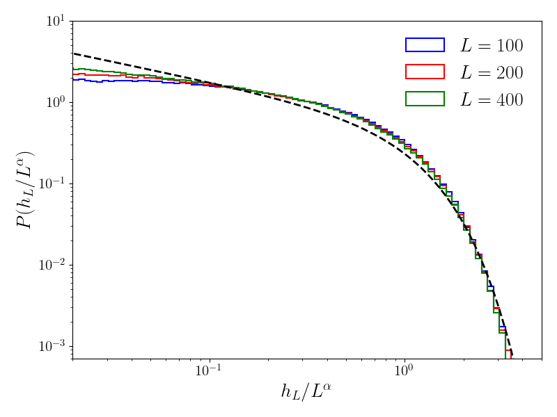
We have shown that when the condition (S105) is satisfied, the mapping between the RW and the stationary SPME is excellent. Now we study cases where the condition (S105) only in the asymptotic limit and deviations are expected when the interface is close to the origin. In particular, this is the case flr the rescaled height for an interface starting at the origin . In Fig. 11, we show that the rescaled height differ from the prediction of the RW, both for and . The behavior is qualitatively correct, but even at and , we are still far from the asymptotic prediction, presumably because is not large enough (in particular for , since ).
In Fig. 12, we also study the distribution of the height differences for for which the multifractal behavior of is expected. We correctly recover the behavior of the typical height difference and its cutoff . The power law decay, predicted in (S83), is underestimated as we find instead of . Larger interfaces are needed to reach the asymptotic limit.
V.3 Structure Factor
The structure factor is a crucial measure that probes the spatial correlations of interface heights. It is defined as:
| (S107) |
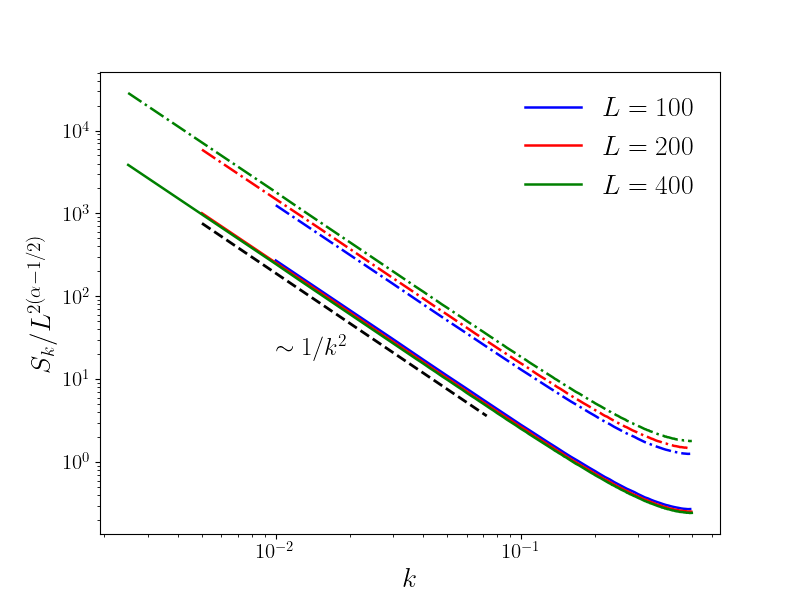
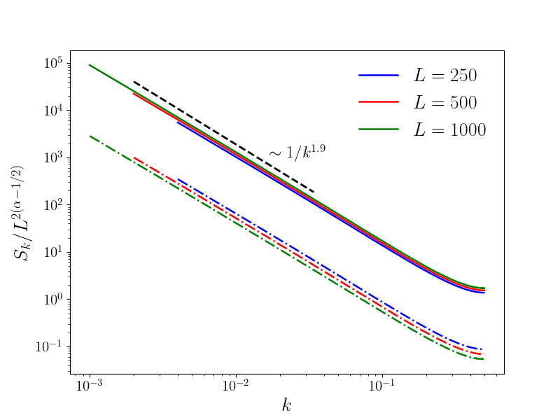
where denotes the Fourier transform of the height profile . The standard scaling behavior in the stationary regime is where is the spatial dimension and the roughness exponent. However, from the mapping to the random walk, we expect the SPME to display anomalous scaling properties. This leads to the prediction, for ,
| (S108) |
with for all since . We thus expect:
| (S109) |
for . This can be seen in Fig. 13. For (Left), this scaling is satisfied. For , the collapse for several improves as increases and the slope is , slightly smaller than the predicted . This is likely due to the finite size effects already observed in the distribution of the jumps in Fig. 12.
VI Fokker-Planck equation for the discrete PME
Consider the discrete SPME equation, for
| (S110) |
and recall that we choose to i.i.d white noises with . We focus here on the case where is fixed and free, which amounts to set .
Denoting the probability density function evolves according to the Fokker-Planck equation
| (S111) | |||
| (S112) |
where is the current. The current vanishes exactly when detailed balance is obeyed, which is not the case here since we are dealing with a non equilibrium system.
With the above boundary conditions, our trial ansatz for the stationary measure corresponds to the probability distribution of for the RW model introduced in the text (S56). We recall that it is defined by the recursion
| (S113) |
This leads to the probability distribution of . It reads with
| (S114) |
We will thus take this trial probability as our initial condition, and see how it evolves. Hence we consider the evolution of starting from
| (S115) |
The current at time is then, for
| (S116) |
with and . One can check that does not vanish exactly for finite , hence the trial ansatz is not an exact stationary measure for finite . However we claim that it becomes an increasingly good approximation of the true stationary measure of the SPME in the large limit upon some appropriate rescaling. This is strongly supported by our numerical simulations and we now provide a rationale for this claim.
It turns out that one can compute exactly the time derivative (at time ) of certain observables with the initial condition given by the trial stationary measure.
Consider an observable and define . One has, for general initial condition
| (S117) |
Applying this at with the initial condition (S115)
| (S118) |
where here we denote by denote an expectation value with respect to our trial measure (S114). Hence (S118) gives a formula for the time derivative at time zero of observables when the system starts at time zero with the trial stationary measure.
Let us consider the observable where is given. For the RW model, and hence at here, from (S113) we see that it corresponds to the increment , which is of order and independent of for . One can thus, at , rewrite:
| (S119) |
One also has:
| (S120) |
One obtains the sum in (S118) as a sum of two terms
| (S121) |
The first one is
| (S122) | |||
| (S123) |
where we have used (S113), (S119), since we are computing expectation values at time with respect to the random walk. We also used that is independent of and is a standard centered Gaussian random variable, hence . The second one is
| (S124) |
since is independent of the other variables and .
In total we have shown that, starting from initial condition one has
| (S125) |
This is not zero, as it would be if the trial distribution was the exact stationary measure.
However we now show that the r.h.s of (S125) vanishes at large as a power of . To determine this power let us choose of order and consider the the probability distribution of . We need to evaluate
| (S126) |
To take into account that there is a cutoff region at , with a finite we can use as an example the form . As we discussed in Section III for the distribution takes the scaling form , which furthermore displays a power law behavior for . Hence the above integral contains two separate regions, and there are two cases.
(i) for the integral is dominated by the region and the integral behaves as
| (S127) |
(ii) for the integral is dominated by the region and the integral behaves as
| (S128) |
At the transition between the two cases i.e. for the decay is .
In summary we have shown that, starting from the random walk probability measure there is an observable which is of order at and whose time derivative vanishes at time zero in the limit of a large system . This is a strong indication that the random walk measure describes well the stationary state of the SPME. Of course it is not a proof, unless we could show that a similar result holds for a much larger class of observable.
Remark. For some observables the time derivative at time zero vanishes exactly. Indeed, let us return to (S118) for a general observable. It reads
| (S129) |
An immediate consequence is that the time derivative (at time zero) of any function of the height at one point, for a given , vanishes since
| (S130) |
Hence the one point marginal distribution of is unchanged in an infinitesimal time interval starting from .