The Steady-State Multi-TeV Diffuse Gamma-Ray Emission Predicted with GALPROP and Prospects for the Cherenkov Telescope Array
Abstract
Cosmic Rays (CRs) interact with the diffuse gas, radiation, and magnetic fields in the interstellar medium (ISM) to produce electromagnetic emissions that are a significant component of the all-sky flux across a broad wavelength range. The Fermi Large Area Telescope (LAT) has measured these emissions at GeV -ray energies with high statistics. Meanwhile, the High-Energy Stereoscopic System (H.E.S.S.) telescope array has observed large-scale Galactic diffuse emission in the TeV -ray energy range. The emissions observed at GeV and TeV energies are connected by the common origin of the CR particles injected by the sources, but the energy dependence of the mixture from the general ISM (true ‘diffuse’), those emanating from the relatively nearby interstellar space about the sources, and the sources themselves, is not well understood. In this paper, we investigate predictions of the broadband emissions using the GALPROP code over a grid of steady-state 3D models that include variations over CR sources, and other ISM target distributions. We compare, in particular, the model predictions in the VHE (100 GeV) -ray range with the H.E.S.S. Galactic plane survey (HGPS) after carefully subtracting emission from catalogued -ray sources. Accounting for the unresolved source contribution, and the systematic uncertainty of the HGPS, we find that the GALPROP model predictions agree with lower estimates for the HGPS source-subtracted diffuse flux. We discuss the implications of the modelling results for interpretation of data from the next generation Cherenkov Telescope Array (CTA).
keywords:
gamma-rays: diffuse backgrounds – Galaxy: structure – ISM: cosmic rays – ISM: magnetic fields1 Introduction
Cosmic ray particles are injected by sources, propagating over millions of years and eventually pervading the Galaxy. This process results in a ‘sea’ of CRs that produce broadband all-sky emissions due to energy losses with the other components of the diffuse ISM: the interstellar gas, the interstellar radiation field (ISRF), and the Galactic magnetic field (GMF). The leakage into the ISM from the individual CR sources also produces localised enhancements of the particle intensities on top of the background ‘sea’, which also contribute to the broadband non-thermal sky brightness. The diffuse emissions by the CRs therefore encode critical information on their sources, how they are injected into the ISM and their propagation history, as well as the spatial distributions of the other ISM components. Observations of their non-thermal emissions can be used to provide essential insights for understanding how the CRs are accelerated up to the highest energies within the Galaxy.
At GeV -ray energies the sky is dominated by the emissions produced by the CR sea throughout the Milky Way (MW), which have been measured and studied extensively with the Fermi–LAT (Ackermann et al., 2012). Recovering individual CR source characteristics at these energies relies on extracting them from the much brighter diffuse fore-/background emissions that they are embedded within. Determination of these fore-/background emissions using a physically motivated methodology is desirable as it enables a more reliable estimate of the true source characteristics. Furthermore, residuals resulting from the subtraction of the fore-/background emissions can be interpreted as true features of physical interest. Generally, analyses of the Fermi–LAT data employ physically motivated interstellar emissions models (IEMs) based on gas tracers and other templates modelled using the GALPROP code (e.g. Acero et al., 2016a; Ajello et al., 2016; Acero et al., 2016b). Systematic studies using such IEMs have been employed for extracting source properties, in particular, for various supernova remnants (SNRs) that are the putative major CR source class (Acero et al., 2016b).
For the VHE range, the emissions about source regions are brighter than the diffuse emission. The recent release of the H.E.S.S. Galactic plane survey (Abdalla et al., 2018) shows localised, extended regions embedded in lower-intensity, broadly distributed emissions – similar to but not exactly the same as the Fermi–LAT data at lower energies. This is due to combined effects. The VHE CRs are more concentrated about the sources. Also, H.E.S.S. uses ‘off source’ fields for background estimation, which likely removes some diffuse emissions and does not enable probing lower fluxes. Recovering source properties for dimmer sources requires proper assessment and accounting for the diffuse emissions.
The VHE diffuse emission is currently observed with low significance by H.E.S.S. (Abramowski et al., 2014), and the spectral extrapolation of a Fermi–LAT IEM indicates a general compatibility with the TeV flux observed by ARGO-YBJ (Bartoli et al., 2015). There is a connection between the GeV and TeV energy ranges, but the energy dependence of the mixture of emissions from the general ISM (true ‘diffuse’), those emanating from the relatively nearby interstellar space about the sources, and the sources themselves, is not well understood. Looking forward, accurately determining their relative contributions will be essential for the next generation of facilities that will have a significantly enhanced sensitivity. An example is the Cherenkov Telescope Array (CTA; CTA Consortium et al., 2019), which is currently under construction.
CTA will have a much larger field of view (10∘) than H.E.S.S., an improved angular resolution (by a factor 5), and will be at least an order of magnitude more sensitive (Actis et al., 2011). The lower flux levels that CTA will reach, and its much larger field of view, will make it extremely sensitive to the details of the diffuse emissions. CTA will also detect hundreds of new -ray sources. Consequently, source confusion, together with the other emissions, will likely be a significant issue that will need to be addressed. Distinguishing between the diffuse and general ISM related emissions, and extended emission coming from the 10s–100s pcs region surrounding the sources, will be critical for accurate recovery of the embedded source properties (Dubus et al., 2013; Acero et al., 2013; Ambrogi et al., 2016).
In this paper, we use the GALPROP CR propagation package to model the diffuse emission into the VHE range for a grid of models that are categorised by CR source density and ISM target density distributions. The models are all spatially 3D and the CR intensity distributions through the ISM are solved for the steady-state case with the propagation parameters optimised to reproduce local CR data. We compare the model predictions with the HGPS observations, carefully accounting for the survey characteristics. We investigate the variation of the predictions for the diffuse emissions across this model grid and use it to estimate the modelling uncertainty. The GALPROP predictions are comparable to lower limits on the diffuse emission at TeV energies inferred from the HGPS observations, when accounting for current estimates of the unresolved source fraction in the data. We discuss also how the accurate modelling of the diffuse emissions and creation of TeV IEMs will be a critical element for maximising the scientific return from the more sensitive observations by facilities such as CTA.
2 GALPROP Modelling
The GALPROP framework (Strong & Moskalenko, 1998; Moskalenko & Strong, 1998) is a widely employed CR propagation package that now has over 25 years of development behind it. For this paper, we use the latest release (v57), where an extensive description of the current features is given by Porter et al. (2022).
2.1 Model Setup
For an assumed propagation phenomenology, the critical inputs for a GALPROP run are the CR source density distribution, together with the distributions of the other ISM components that result in the energy losses and corresponding secondary particle and emissions production. The CR source distribution is subject to considerable uncertainty, and we construct a representative set of 3D models varying the respective content of sources distributed in the Galactic disc and spiral arms. Meanwhile, GALPROP has well developed 3D models for the interstellar gas and radiation fields, and a collection of GMF models taken from the literature. We fix the interstellar gas model and make predictions for combinations of the interstellar radiation and magnetic field distributions over the CR source density distributions. We describe in detail below these elements for our calculations.
2.1.1 The Interstellar Gas
The ISM gas consists mostly of H and He with a ratio of 10:1 by number (Ferrière, 2001). It can be found in the different states, atomic (H i), molecular (H2), or ionised (H ii), while He is mostly neutral. H i is 60% of the mass, while H2 and H ii contain 25% and 15%, respectively (Ferrière, 2001). The H ii gas has a low number density and scale height few 100 pc. The H2 gas is clumpy and forms high density molecular clouds.
For this paper, we use the 3D gas density distributions for the neutral ISM developed by Jóhannesson et al. (2018). They were obtained using a maximum-likelihood forward model folding method to the LAB H i-survey (Kalberla et al., 2005) and the CfA composite CO survey (Dame et al., 2001). These neutral gas models include a warped and flaring disc, four spiral arms, and a central bulge. For the H ii we employ the NE2001 model (Cordes & Lazio, 2002, 2003; Cordes, 2004) with the updates by Gaensler et al. (2008). The CR energy losses and fragmentation (for nuclei) depend on the spatial density distribution for the interstellar gas.
For calculating gas-related -ray intensities we use the gas column-density maps based on the HI4PI survey (HI4PI Collaboration et al., 2016) and the composite CO survey, with a correction for the contribution of missing so-called ‘dark gas’ (Grenier et al., 2005) using a map of optical depth at 353 GHz based on Planck data (Planck Collaboration et al., 2016). The gas column density maps for atomic and molecular hydrogen are split into Galactocentric radial bins using a rotation curve (Ackermann et al., 2012) due to the limited kinematic resolution of the data. The line-of-sight integration uses the gas density model to accurately weight the CR flux over the extent of the individual rings. This enables the use of the full resolution of the CR intensity solutions that determine the secondary emission emissivities. Helium and heavier elements are assumed to be identically distributed and are accounted for by correction factors.
2.1.2 The CR Source Distributions
While the SNRs are believed to be the principal CR source class, pulsar wind nebulae (PWNe) and other types likely contribute at some level, but the relative amount is poorly known. For the purpose of this paper, we do not specify the individual source classes that are typically given according to 2D Galactocentric averaged distributions (e.g. Ackermann et al., 2012). Instead we construct a set of synthetic distributions with systematic gradation of the proportion between disc and spiral arm components to investigate the effect of the 3D source distribution on the VHE -ray emissions.
We follow Porter et al. (2017) and Jóhannesson et al. (2018) using the disc-like distribution from Yusifov & Küçük (2004) and four spiral arms. The spiral arms have the geometry of those for the R12 ISRF model (see below), but with equal weighting for their normalisations. Our CR source distributions start with a purely disc-like distribution (that we term SA0), and increase with relative contribution by the spiral arms until the distribution is purely due to the spiral arms (termed SA100). Consequently, we have the SA0, SA25, SA50, SA75, and SA100 distributions corresponding to 0, 25, 50, 75, and 100%, respectively, for the source luminosity contained in the spiral arms, with the remaining source luminosity in the disc-like component. The primary CR source spectra and other parameters are determined for each model by the optimisation procedure described below.
2.1.3 The Interstellar Radiation and Magnetic Fields
The CR electrons and positrons lose energy via Compton and synchrotron interactions with the interstellar radiation and magnetic fields. Into the VHE range, these processes strongly influence the CR spectral intensities and correspondingly affect the intensity distribution for the rays. Because there is still uncertainty for the ISRF and GMF distributions, we employ representative models that are available within the GALPROP framework.
The ISRF encompasses the electromagnetic radiation within the Galaxy, including emission from stars, infrared light from interstellar dust radiating heat, and the cosmic microwave background (CMB). The state-of-the-art 3D ISRF models for the MW were developed by Porter et al. (2017) based on spatially smooth stellar and dust models. They have designations R12 and F98 that correspond to the respective references supplying the stellar/dust distributions (Robitaille et al., 2012; Freudenreich, 1998). They similarly reproduce the data, but neither is an overall best match. The R12 model provides better correspondence toward the spiral arm tangents, but does not display the asymmetry associated with the bar (R12 has an axisymmetric stellar bulge), and the stellar disc scale length is incompatible with the near-IR profiles. Meanwhile, the F98 model has the disc scale-length in better agreement with the near-IR data, incorporates the bulge/bar asymmetry, but has none of the structure associated with the spiral arms.
Both R12 and F98 models are providing equivalent solutions for the ISRF distribution. At least toward the inner Galaxy, where the ISRF intensity is most uncertain, they are providing lower and upper bounds as determined by pair-absorption effects on sources toward the Galactic centre (GC) (Porter et al., 2018).
The GMF consists of the large-scale regular (Beuermann et al., 1985) and small-scale random (e.g. Sun et al., 2008) components that are about equal in intensity. The random fields are mostly produced by the SNe and other outflows, which result in randomly oriented fields with a typical spatial scale of 100 pc (Gaensler & Johnston, 1995; Haverkorn et al., 2008). Also, there may be the anisotropic random (‘striated’) fields that are a large-scale ordering originating from stretching or compression of the random field (Beck, 2001). This component is expected to be aligned to the large-scale regular field, with frequent reversal of its direction on small scales. GALPROP includes multiple large-scale MW GMF models (Sun et al., 2008; Sun & Reich, 2010; Pshirkov et al., 2011; Jansson & Farrar, 2012; Jaffe et al., 2010).
In this paper we use the bisymmetric spiral GMF model from Pshirkov et al. (2011), that we refer to as PBSS, as a representative model with a spiral structure. We also employ the GALPROP axisymmetric exponential distribution (GASE; Strong et al., 2000). It has the functional form for Galactocentric coordinates :
| (1) |
where is the magnetic field strength, kpc is the IAU recommended distance from the GC to Earth (Kerr & Lynden-Bell, 1986), and kpc and kpc are the scale heights for the radial and height components, respectively. This distribution is a simple, exponentially decreasing field in both Galactocentric radius and height above the plane, and does not include the spiral arms. Although there are more modern GMF distributions that have better agreement with radio data, including those mentioned above, the GASE GMF is still commonly used throughout the literature (e.g. Korsmeier & Cuoco, 2022; Qiao et al., 2022). The use of the GASE GMF in this work is therefore to allow us to better characterise the variation between commonly used GMF distributions.
2.1.4 Parameter Optimisation
For this paper we assume a diffusive-reacceleration propagation model with isotropic and homogeneous spatial diffusion coefficient111Note that the spatial diffusion coefficient for the CR propagation can be linked to the GMF strength distribution in GALPROP (Ackermann et al., 2015), but we do not use this functionality for the present paper.. The consistency condition is that each combination of the inputs described above reproduces the local CR spectra. To ensure this, we optimise the propagation parameters and source spectra as described below.
The CR propagation calculations use a 3D right-handed spatial grid with the solar system on the positive -axis and kpc defining the Galactic plane with kpc for the distance from the Sun to the GC. For runtime efficiency we use the non-uniform grid functionality included with the v57 GALPROP release (Porter et al., 2022) for solving the propagation equations. We employ the tangent grid function where the parameters for the transformation function are chosen so that the resolution nearby the solar system is 30 pc, increasing to 1.2 kpc at the boundary of the Galactic disc, which is at 20 kpc from the GC. In the -direction the resolution is 15 pc in the plane, increasing to 0.6 kpc at the boundary of the grid at kpc (Jóhannesson et al., 2016). The kinetic energy grid is logarithmic from 1 GeV to 1 PeV with ten planes per decade.
We follow the procedure in Porter et al. (2017) and Jóhannesson et al. (2018), with the CR data from Jóhannesson et al. (2019) (see their table 1). For each of the source distributions, an initial optimisation of the propagation models is made by fitting to the observed CR spectra from AMS-02 and Voyager 1 in the GeV energy range, where the CR sea is the dominant source of CRs. This procedure is performed for the CR species: Be, B, C, O, Mg, Ne, and Si. These are kept fixed, and the injection spectra for electrons, protons, and He are tuned together. As the proton spectrum impacts the normalisation of the heavier species, and therefore also impacts their propagation parameters, this process is performed iteratively until convergence. As we are extrapolating outside the energy range of the data, the best-fit model for the source distributions is determined via a test, and then its local CR spectra are used to re-optimise the CR data for the other source distributions. This is to ensure that all five source distributions give the same local CR spectra, reducing inconsistences between the distributions due to limited data statistics and coverage over the modelled energy range. Examples between the model and data agreement are provided in Porter et al. (2017) up to 1 TeV/nucleon. For higher energies, the spread of the observations is larger, and a range of spectral indices can be consistent with the measurements. For example, for protons with energies around GeV the difference between experiments in the measured fluxes with uncertainties is approximately an order of magnitude (Choi et al., 2022). The parameters that vary with the source distributions are shown in Table 1.
The CR injection spectra are given by the power-law with two spectral breaks, and is defined separately for electrons, protons, Helium, and a single spectral form for all CR species heavier than Helium. The proton and electron spectra are normalised at the Solar position to and at the energies GeV and GeV respectively, with heavier elements normalised relative to the proton spectrum at 100 GeV/nuc. The CR spectral breaks are given by the rigidities and , and the spectral indices are given by for rigidities , for rigidities , and for rigidities . The diffusion coefficient is given by the power-law , and is normalised to at the rigidity GV with the spectral index given by . The normalisation rigidity, spectral breaks, and spectral index after the break are held constant across all models. Finally, as the -ray spectrum at a given energy always depends on more energetic CRs, we set the nuclei cut-off energy () to 1 PeV/nuclei across all models to ensure the correct treatment of the -ray spectrum up to 100 TeV.
Although there are hints for a cut off in the local (i.e. post propagation) electron spectrum above 10 TeV (e.g. Aharonian et al., 2009; DAMPE Collaboration et al., 2017), local measurements are unable to constrain the CR electron spectrum across the entire MW due to the short (1 kpc) travel distances of multi-TeV electrons. As electrons are known to be accelerated in the MW up to PeV energies by PWNe, no artificial cut off is applied to the CR electron injection spectrum for our models.
| Parameter | SA0 | SA25 | SA50 | SA75 | SA100 |
|---|---|---|---|---|---|
| [] | 4.36 | 4.39 | 4.55 | 4.67 | 4.66 |
| 0.354 | 0.349 | 0.344 | 0.340 | 0.339 | |
| 17.8 | 18.2 | 18.1 | 19.8 | 19.1 | |
| [] | 4.096 | 4.404 | 4.113 | 4.329 | 4.394 |
| [] | 3.925 | 4.444 | 3.994 | 4.428 | 4.502 |
| 1.616 | 1.390 | 1.488 | 1.455 | 1.521 | |
| 2.843 | 2.756 | 2.766 | 2.763 | 2.753 | |
| 2.493 | 2.460 | 2.470 | 2.447 | 2.422 | |
| 6.72 | 5.27 | 5.14 | 5.54 | 5.29 | |
| 52.4 | 81.6 | 67.7 | 70.7 | 79.7 | |
| 1.958 | 1.928 | 1.990 | 1.965 | 2.009 | |
| 2.450 | 2.464 | 2.466 | 2.494 | 2.481 | |
| 2.391 | 2.411 | 2.355 | 2.374 | 2.414 | |
| 12.0 | 12.3 | 12.2 | 14.5 | 13.5 | |
| 202 | 157 | 266 | 108 | 125 | |
| 1.925 | 1.886 | 1.956 | 1.937 | 1.971 | |
| 2.417 | 2.421 | 2.432 | 2.467 | 2.443 | |
| 2.358 | 2.369 | 2.320 | 2.347 | 2.376 | |
| 12.0 | 12.3 | 12.2 | 14.5 | 13.5 | |
| 202 | 157 | 266 | 108 | 125 | |
| 1.328 | 1.519 | 1.426 | 1.630 | 1.624 | |
| 2.377 | 2.390 | 2.399 | 2.399 | 2.418 | |
| 2.377 | 2.390 | 2.399 | 2.399 | 2.418 | |
| 3.16 | 4.21 | 3.44 | 4.61 | 4.50 | |
| [] | 5.00 | 5.00 | 5.00 | 5.00 | 5.00 |
is the power-law index before the first break, between the first and second, and after the second break.
[GV] is the rigidity of the first break, and [GV] is the rigidity of the second break.
The diffusion coefficient () is measured in cm2 s-1, the Alfven velocity () in km s-1, and the CR normalisation constants ( and ) are measured in MeV-1 cm-2 s-1 sr-1.
2.2 Interstellar Emissions Modelling Predictions
The propagation model parameters for each source distribution (Table 1) are used to calculate steady-state CR intensity solutions across the Galaxy using GALPROP. The spatial grid used for the CR propagation calculations is also employed for determining -ray emissivities. The -ray intensity maps at the solar system location are obtained by line-of-sight (LOS) integration of the -ray emissivities for the standard processes (-decay, IC scattering), where the emissivities are determined for a logarithmic grid from 1 GeV to 100 TeV using five bins per decade spacing. We use a HEALPix (Górski et al., 2005) order 9 isopixelisation for the skymap generation222This gives a pixel size of , which is similar to the point-spread function of H.E.S.S. ().. All calculations of the IC component use the anisotropic scattering cross section (Moskalenko & Strong, 2000), which accounts for the full directional intensity distribution for the R12/F98 ISRF models. The attenuation that affects the -ray intensities mainly 10 TeV, is included in the LOS integration, where the optical depth calculation includes the directionality of the ISRF (Moskalenko et al., 2006; Porter et al., 2018). For the R12/F98 ISRF models, the relevant precomputed optical depth maps included with the v57 GALPROP release are employed.
Fig. 1 shows the predicted fluxes from 1 GeV to 100 TeV averaged over different Galactic quadrants about the plane and within of the north/south polar regions. For clarity, we show only the modelled fluxes for the SA0 and SA100 distributions for the R12/PBSS ISRF/GMF combination (other combinations display qualitatively similar trends). Along the plane, for the central longitudes () and central latitudes () the IC emission starts to account for a large fraction of the total -ray emission around 100 GeV, and dominates the TeV Galactic emission after 10 TeV, for all source distributions. For the outer-Galactic region, where there are fewer CR sources (), the IC provides a strong relative contribution until 10 TeV energies, when there is less variation overall between the SA distributions. Meanwhile, towards the polar regions () there is a much lower column density for the ISM gas, which results in a reduction of the -decay emissions intensity. Because the scale height of the ISRF is larger than that of the gas, the IC emission is reduced to a lesser degree over these parts of the sky. This results in it being the strongest component of the -ray sky brightness for all SA distributions across the entire spectrum, from 1 GeV to 100 TeV.


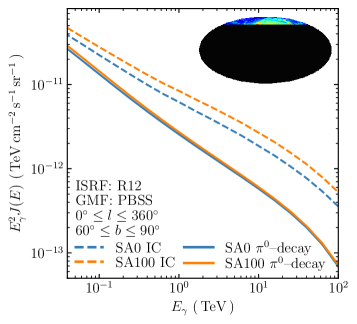


Fig. 2 shows the total flux for the various SA distributions averaged over the HGPS analysis region ( and ). As the cooling time for VHE CR electrons is short, the impact of the source distribution is most easily seen for the IC emission contribution. Source density distributions with a higher weighting for CR sources in the arms generally boost the IC signal. This is due to the greater concentration of CR injection about the arms together with the higher ISRF/GMF densities that are also similar in distribution to the sources. This ‘density squared’ effect (Porter et al., 2017) enhances the emissions over the more smoothly distributed model combinations. The impact is such that for the SA100 distribution the IC flux at 100 TeV is a factor 2 brighter than that from the SA0 distribution.

Enhancements due to the ISRF distribution mainly affect the IC emissions for energies 10 TeV. In Fig. 3 we show predicted fluxes over the HGPS region with variation for the ISRF model. Below 100 GeV the stronger optical ISRF about the spiral arms in the R12 model enhances the IC emissions when compared to the F98 model. At higher energies the Klein-Nishina (KN) suppression reduces this effect, and the predictions for both become closer due to how the IR component of the respective ISRF models is distributed relative to the CR electrons. For energies 1–2 TeV the IC emission for the SA0 distribution varies 10% between the R12 and F98 ISRFs, while there is little variation switching between the ISRF models for the SA100 distribution. This variation for the SA0 distribution is due to the peaking of the source density about the GC. There is a correspondingly higher electron intensity across the inner Galaxy that can produce IC emissions. While for the SA100 distribution there is little variation as the inner cut-off for the spiral arms effectively produces a central ‘hole’ in the electron intensity distribution. Therefore, there is much less IC emission coming from the inner Galaxy for this source density distribution. For energies 10 TeV even the IR component becomes KN supressed as well, and only scattering of the CMB is contributing to the emission. The result is a negligible difference between the ISRF models at higher energies, where the different predictions is due solely to the varying source density distributions.

Fig. 4 shows the variation of the IC flux when the GMF model is varied for fixed ISRF distribution. Varying the GMF distribution has a significant effect on the IC emission as energy increases into the VHE range due to the synchrotron losses dominating the cooling time scale for the electrons. At 1 TeV the difference in the IC emission between the PBSS and GASE distributions is approximately 30%, increasing to 100% by 100 TeV. For synchrotron emission, the energy radiated by TeV electrons over time () is proportional to the square of the magnetic field strength () of the medium that they diffuse through and the energy of the particle, i.e. . As the radiative losses of electrons depends strongly on the magnetic field strength, regions with higher GMF energy density will rapidly be depleted of high energy electrons. The GASE distribution has the most intense region of the field at the GC, leading to the IC emission being greatly reduced in the GC when compared to the PBSS distribution.

Fig. 5 shows the longitudinal profile of the IC and -decay emission for the various source distributions for energy levels between 0.1 TeV and 100 TeV. The -decay dominates the -ray emission for all longitudes for the energies 1 TeV. Because the energy losses for CR nuclei are slow and the diffusion is relatively fast, the propagated distributions for them are fairly smoothly distributed over all source distributions. There is, correspondingly, minimal impact on the -decay component in the longitudinal profiles. Meanwhile, the IC emission becomes dominant for 10 TeV energies. Because the energy losses are much faster for the electrons, its contribution to the profiles is much more sensitive to changes in the source distribution over most of the Galactic plane. As the majority of the spiral arms are located between Earth and the GC, with one of the arms located in close proximity to the Earth, we see that for a larger fraction of CRs being injected into the spiral arms (e.g. SA100) the IC component becomes more intense for the central region (i.e. ). The IC emission is also boosted along the spiral arm tangents located at . For the negative longitudes between the anti-centre and perpendicular to the GC, i.e. for , the IC emission decreases with an increasing fraction of CR injection in the spiral arms, and the difference between the source density distributions increases with increasing energy.
Across the entire plane for all source distributions the IC emission dominates the -ray emission at 100 TeV. It is not a surprise that the spiral structure in the source density distributions including arms is evident in the profiles. However, at these energies there also appears to be structure for the SA0 density distribution IC profile similar to those models including arms that is not apparent at lower energies. Because of the KN suppression for the optical and IR components of the ISRF, the only photon field is the (uniform) CMB for IC processes. The energy density of the GMF varies, but is much higher than that for the CMB about the spiral arms, and hence determines the energy loss time scale affecting the electron distribution. The observed structure in the 100 TeV IC profile for the SA0 distribution is therefore entirely due to that encoded in the PBSS GMF distribution, with its influence imprinted on the electron energy density.
For the spiral arms in the source distributions, the closest arm in the sky region is the Perseus arm located 3 kpc away. For the source distributions with a high fraction of CR injection in the spiral arms (e.g. SA75 and SA100), there is a large void of electron sources between the Solar System and the Perseus arm, resulting in reduced TeV IC emission in that direction. However, as the Galactic disc component of the source distributions is smoothly varying, the source distributions with a low fraction of CR injection in the spiral arms (e.g. SA0 and SA25) have boosted TeV IC emission in these regions, as CRs are injected in the voids between the Solar System and the Perseus arm. This is not seen in the positive longitudes far from the GC ( ) as the Perseus arm is close enough to the Solar System such that there is no void in the electron densities in any of the source distributions. The proximity of the Perseus arm leads to a lower degree of variation in the IC emission in this region of the Galactic plane across the SA distributions. Figs. 4 and 5 therefore show that the source distributions with a larger fraction of sources in the spiral arms show increased IC emission along the arm tangents, with the IC emission dominating over the pion-decay at 1 TeV along the arms.

Fig. 6 shows the envelope of longitudinal profiles at 1 TeV of all the GALPROP runs across our model grid, i.e. any combination of the source distribution, ISRF, and GMF. Due to using a mix of distributions that include the spiral arms and those that do not (e.g. combining the SA0 with the PBSS distribution), no single GALPROP run describes the lower or upper bound of the envelope. However, from the upper/lower bounds we infer that there is a % variation over the entire grid of GALPROP predictions for models that are consistent with the local CR data. Changing the source distribution alone tends to alter the longitudinal profile most significantly toward the spiral arm tangents, where the variation can be up to 40% when comparing SA0 to SA100. Toward the inner Galaxy there are smaller differences, due to both the lower number of sources about the GC for distributions with spiral arms, and to the smoothing from the LOS integration over the long path lengths for these directions. For similar reasons, changing the ISRF model impacts the results only modestly (up to 4%) around the central plane . Meanwhile, changing the GMF model has the strongest effect around the central where the impact can be up to 20% variation. We show overlaid in Fig. 6 two individual results – one with no spiral arms in the CR injection distribution, ISRF, or GMF (i.e. the SA0, F98, and GASE configuration), and the other having spiral arms in all three (i.e. the SA100, R12, and PBSS configuration). The variation between the predictions is generally driven by the increasingly complex 3D structures for the respective components of the models that we have considered.
3 Comparing the HGPS to GALPROP
The HGPS represents the most comprehensive survey of the Galactic plane at TeV energies to date. Extraction of an estimate for the HGPS diffuse contribution requires accounting for the treatment of the CR background in the data. For this H.E.S.S. used the adaptive ring method, with a set of exclusion zones that cover approximately two thirds of the Galactic plane, such that no -ray sources are considered as part of the CR background estimate. However, this may subtract the diffuse rays that are captured in the background regions. The HGPS observations also include both discrete and unresolved sources, neither of which are part of the diffuse emission. We briefly describe how we address these issues below, with the full details given in Appendix A.
Our analysis of the HGPS uses the survey sky map with an integration/containment radius of such that we are as sensitive as possible to the TeV diffuse -ray emission. We then use a sliding window method with parameters suitably optimised to reveal the longitudinal structure of the diffuse emission (see Appendix A). The sliding window is applied after the masking of known catalogued sources, which either subtracts the catalogued source component of the emission or excludes the catalogued source region from the analysis. It is also necessary to account for the unresolved sources, i.e. the ensemble of -ray sources below the detection threshold of H.E.S.S.. Although they are not individually resolved, these unresolved sources still contribute to the total observed Galactic emission, providing an extended low surface brightness contribution to the observed flux. As they are not part of the truly diffuse emission, their contribution must be subtracted. We use estimates for the unresolved source component from Steppa & Egberts (2020) (SE20) and Cataldo et al. (2020) (C20) who give relative contributions to the HGPS of 13%–32% and 60%, respectively. We combine them with the systematic uncertainty in the H.E.S.S. fluxes to provide lower and upper limits for the diffuse -ray emission.
Fig. 7 shows the source-subtracted flux obtained with our method, together with the bounding estimates employing the different unresolved source contributions. This is shown together with the longitudinal profile of the HGPS sensitivity in units of %Crab333Units of %Crab are generally used in VHE -ray astronomy. We use the definition (Aharonian et al., 2006). There is a large-scale -ray emission along the plane, similar to that found previously by Abramowski et al. (2014). Its brightness varies over the survey area, with the lowest level 2–3 times below the point source sensitivity of the HGPS.

We apply the same sliding window procedure to the GALPROP predictions over our model grid (Section 2) to enable a comparison with the HGPS diffuse flux estimates. Our GALPROP results were converted into units of %Crab deg-2 to allow comparisons to the HGPS sensitivity, which is given in units of %Crab. As GALPROP predicts only the diffuse interstellar emissions, the masking of catalogued and subtracting of the unresolved source component is not required. Fig. 8 shows the comparison between the HGPS longitudinal profile for the range of the GALPROP predictions (see Fig. 6) after the averaging window has been applied. Also shown are the HGPS estimates with subtraction of the SE20 and C20 unresolved source fractions and HGPS sensitivity profile.

Our GALPROP-based models generally underpredict the large-scale TeV emission estimated from the HGPS. This is due to the HGPS data containing a large number of unresolved sources that artificially inflate the large-scale emission to levels above the TeV diffuse emission. Subtracting the unresolved sources from the large-scale emission via the estimates from SE20 or C20 provides a lower limit on the Galactic diffuse TeV emission. Accounting for this contribution, the GALPROP predictions broadly agree with the diffuse -ray emission estimate obtained by subtracting an unresolved source fraction from C20. However, this is not true across the whole longitude range where, e.g. around , we can find better agreement with estimated diffuse flux using the unresolved source fraction from SE20. It is therefore likely that the unresolved source contribution lies between those determined by SE20 and C20 across the region spanned by the survey, but it is not clear where either of the models is most applicable.
For Galactic longitudes the GALPROP predictions are below the lower-limit for the TeV diffuse emission. However, this region of the Galactic plane is well below the sensitivity of the HGPS, making it difficult to draw any conclusions on the diffuse emission. The disagreement could be due to poor statistics in the region, or that the GALPROP models are insufficiently optimised toward these directions.
4 Discussion
4.1 Interstellar Emission Model Predictions into the TeV Energy Range
Our work is the first systematic study using the GALPROP framework to predict the diffuse emissions into the TeV energy range for a grid of physical modelling configurations. For the steady-state models that we have considered, generally the -decay component produced by the CR nuclei interactions with the interstellar gas has only a small variation over the HGPS survey area (Fig. 2). Because the energy losses of these CRs are slow, they are distributed fairly smoothly across the MW with only mild imprints of the source density distribution. However, this is not the case for the IC emissions. Averaged over the HGPS survey area there is a much stronger variation due to the choice of source distribution. The energy losses for the CR electrons are much more rapid than those for the nuclei. The concentration of the ISRF and GMF energy densities about the spiral arms combines to affect the -ray intensities toward those regions, because they approximately coincide toward where the source densities with arms tend to also be enhanced. Into the TeV energy range, the IC emissions have much higher sensitivity to the ISRF and GMF energy density distributions.
There are three composite source density distributions in our source density model grid (both Galactic disc and spiral arm components: SA25, SA50, and SA75). For a fixed target density distribution (i.e. holding the ISRF/GMF constant), comparing the 1 TeV -ray longitudinal profiles for these three composite source density distributions shows a variation of 10%. When comparing all five source density distributions, we find a much larger variation up to 50%. Altering the target densities as well as the source density distributions, as is done in Fig. 6, shows a variation up to 100%. The effect of progressively more complex 3D structures for the source density and ISRF/GMF components leads to more variation for the TeV emissions from the CR electrons for the propagation model phenomenology that we have used in this paper. However, the envelope of model predictions resulting from variations in the target densities is larger than that from solely changing the source density distribution. While our current understanding of the spatial distributions of the ISM components that are the targets for producing the VHE emissions is incomplete, we have used models for them that are reasonably agreeing with data. The GALPROP predictions from our study are therefore representative of the likely uncertainty associated with current modelling for the VHE diffuse emissions.
We have used a grid of source density models where the normalisation is obtained by requiring consistency of the propagated CR intensity distributions with the data obtained at the solar system. This is a well-motivated normalisation condition, given the considerable uncertainties associated with correctly defining CR source population characteristics. However, there is an effective CR ‘horizon’ beyond which additional components may be added without any noticeable effect when normalising to the local CR data. For example, CRs injected about the GC likely have a negligible impact on the intensities at the solar system location. Correspondingly, a source density localised about the inner Galaxy, e.g. distributed similar to the stellar bulge/bar (Porter et al., 2017; Macias et al., 2019), will have its injected CR power as a free parameter. Such additions localised about the inner Galaxy require tuning at other frequencies, e.g. the GeV energy data, to correctly optimise parameters for use as a ‘background’ in the VHE regime. While the uncertainty band for the diffuse emissions that we estimated above is below the 5 significance level of the HGPS (see Fig. 8), such additional components have the possibility to also contribute toward the inner Galaxy. At the moment it is likely that a unique solution is not possible for precise estimation of the diffuse background for the HGPS data.
Our modelling has also shown that the IC emissions across the plane starts to become dominant over the -decay above 10 TeV (Fig. 5). The profiles for 10 TeV -ray energies display structure in the leptonic component that is due to the combination of the spatial distributions employed for our models. However, at the higher energies (100 TeV) the situation becomes simpler, because the complications of the uncertainty in the ISRF distribution effectively disappear by the KN suppression of the optical and IR components. Only the GMF and source density distributions are determining the structure visible in the longitudinal profiles for these energies. Currently, the GMF models for the MW are poorly constrained, and are most commonly constructed by using rotation measures of extragalactic sources. Given that the GMF structure is observable at 100 TeV, the future VHE/UHE -ray observations provide an interesting possibility to constrain the GMF configurations. However, -ray emission is created by the convolution of the source density distribution and the target density distributions. The alignment of the GMF and source density distribution is not complete, which is not surprising given that the different tracers for the Galactic spiral structure show offsets (e.g. Vallée, 2020). Therefore using -ray observations to constrain the GMF will likely require -ray facilities many times more sensitive than what is currently available.
We note that for this paper we have only considered steady-state models. Into the TeV energy range the time-dependent solutions, particularly for the CR electrons, are likely necessary (Porter et al., 2019). For example, the Tibet AS data indicate that many of the rays detected within their , window (Amenomori et al., 2021) are not close on the sky to known VHE -ray sources. The observational data from Tibet AS appears inconsistent with the simple models of Lipari & Vernetto (2018) and Cataldo et al. (2019)444These efforts do not use propagation codes, instead employing simple parametrizations for the CR spectra assuming steady-state conditions, and do not consider the 3D structure of the CR sources and ISM., and a discrete origin has been suggested (e.g. Dzhatdoev, 2021; Fang & Murase, 2021). Recent results from Vecchiotti et al. (2022) found that the discrepancy between models and the Tibet AS flux could be due to a population of unresolved PWNe, which would likely increase the leptonic component of the TeV rays. PWN halos have also been proposed as a large contributor to the unresolved sources for both H.E.S.S. and HAWC (Martin et al., 2022), further suggesting that electrons contribute to the diffuse emission. The increasing contribution by the leptonic component with energy that we have shown in this paper, and its likely significant fluctuations, may help explain the lack of correlation between the PeV rays observed by Tibet AS and neutrinos seen along the Galactic plane. We also have results from HAWC (Abeysekara et al., 2017) and LHAASO (Zhao et al., 2021) that show for energies 10 TeV the localisation of emissions about individual sources is stronger. Incorporating time-evolution into the modelling seems to be necessary next step to accurately connect the GeV to 100s TeV energies emissions that are presumably coming from a common origin.
4.2 Application to CTA and Other TeV Facilities
CTA will perform a Galactic plane survey (GPS) over its first ten years of operation, which will cover Galactic latitudes in the range and all Galactic longitudes, averaging 32 hours of observation per square degree (CTA Consortium et al., 2019). The CTA GPS will have an energy range from 100 GeV to 100 TeV, with a resolution of around for energies above 1 TeV. The point source sensitivity of CTA’s proposed 10-year survey will reach 1.8 mCrab for the inner and 3.8 mCrab for the outer Galactic longitudes. For comparison, the HGPS has a point source sensitivity of 4–20 mCrab between with an average of 146 hours of observation per square degree. The sensitivity of the proposed CTA GPS after adjusting for a containment radius of is also shown in Fig. 8.
As CTA is expected to detect and resolve on the order of a thousand of new sources (Actis et al., 2011), these exclusion regions will grow to encapsulate a significant fraction of the Galactic plane, if not the entire plane. Allowing nearby sources to contaminate the background, such as would be very likely along the Galactic plane without careful consideration, would significantly reduce the sensitivity of the observations (Ambrogi et al., 2016).
CTA presents a leap forward in terms of the angular resolution it will achieve, with a PSF reaching approximately for -ray measurements at 1 TeV. The all-sky H i and CO survey data that is used for building the neutral ISM model used in this work have resolutions of and , respectively. This is adequate for comparisons to the HGPS, but not to CTA’s expected Galactic plane survey. New high-resolution ISM surveys, such as Mopra CO (Braiding et al., 2015, 2018) in the Southern hemisphere, and Nobeyama 45m CO (Minamidani et al., 2015; Umemoto et al., 2017) and THOR H i/OH (Beuther et al., 2016; Wang et al., 2020) in the Northern hemisphere have become available. High-resolution ISM surveys that can observe the small, dense clumps at comparable or better angular resolution to CTA will become a necessary modelling ingredient for future high-resolution comparisons to its GPS. Due to the high density of these clumps it will also become necessary to adapt the diffusion coefficient to the density of the ISM gas (e.g. Gabici et al., 2007, 2009).
From Fig. 8 we can see that CTA-South should be able to detect the TeV diffuse -ray emission to the 5 level given even our conservative estimates of the diffuse -ray emission predicted in this paper for the central of longitude (). As has already been seen with the sensitive Fermi-LAT data at lower energies, it will therefore be necessary to develop accurate models for the diffuse emission to separate individual source characteristics from it. This will be essential for resolving and detecting faint, extended TeV emissions such as those such as those expected from PWN haloes, and for probing complex morphological structures of TeV sources. This will potentially allow the identification of currently unidentified sources in the HGPS and other current and future observations, such as those from CTA.
For the Galactic longitudes open to Northern-hemisphere observations, i.e. , our estimates state that the diffuse emission flux at 1 TeV is below 5 mCrab/deg2. This emission is below the extended source sensitivity for CTA-North, which is planned to perform the deepest Galactic plane survey of any IACT in the Northern hemisphere at 1 TeV (CTA Consortium et al., 2019). It is therefore unlikely that any IACT in the Northern hemisphere, such as VERITAS (Vassiliev, 1999) and MAGIC (Aleksić et al., 2012), will observe the diffuse emission. Ground-level particle detectors in the Northern hemisphere, such as LHAASO (Sciascio, 2016), HAWC (Abeysekara et al., 2013), and Tibet AS (Sako et al., 2009), are optimised for multi-TeV to PeV observations. This has allowed Tibet AS to successfully detect extended, presumably diffuse, emission at PeV energies (Amenomori et al., 2021). However, as these particle detectors are optimised for multi-TeV to PeV observations, it is unlikely they will observe this diffuse emission around 1 TeV within their first ten years of operation. The Northern hemisphere detector ARGO-YBJ was constructed to be more sensitive at TeV energies, and has measured the diffuse emission at 1 TeV after five years in the region . The emission predicted by our GALPROP models is within the uncertainty band estimated for these data (Bartoli et al., 2015).
Observation of the Galactic diffuse emission below the PeV regime (e.g. around 1 TeV) will likely remain difficult with the current and the next generation of -ray observatories. For the Southern hemisphere, the planned ground-level particle detector SWGO (Albert et al., 2019) has the possibility of observing the Galactic diffuse emission at 1 TeV around the GC within the first ten years of operation, complementing the higher-resolution CTA-South observations.
5 Summary
We have made a systematic comparison of the predicted diffuse TeV -ray emission over a grid of steady-state models generated using the GALPROP framework. For the models that we consider, the variations in source density, ISRF, and GMF distributions can have a significant effect on the predicted IC emissions at VHEs. The magnitude of the variation on the IC emissions around 1 TeV toward the GC can be 50–60%. This increases to 100% for 100 TeV energies. The influence of differing ISRF distributions is most important for energies 1 TeV, modest for 1–10 TeV, and vanishes 40–50 TeV due to the KN suppression that removes all but the CMB as a target photon field for Compton scattering processes at the highest energies. For energies 20–30 TeV, the CR source density and GMF distributions have the most significant impact on the predicted -ray emissions. Generally the energy losses at VHEs for the CR electrons are most strongly influenced by the GMF distribution. The structure of the GMF is imprinted on the CR electron intensity distribution and hence the VHE diffuse emissions produced by them. This is seen in the IC emissions, with the GMF structure becoming more pronounced as energy increases into the 100 TeV range.
Towards the inner Galaxy () we found that the leptonic component of the diffuse -ray emission begins to become an important consideration around 1 TeV, with the hadronic component dominating for most of the Galactic plane. At 10 TeV the leptonic emission begins to dominate over the hadronic emission for the inner Galaxy, while the leptonic component is approximately equal in magnitude to the hadronic emission for the region (). For the 100 TeV energy range, our results show that the IC emission dominates the total diffuse -ray emission across the entire plane for all models that we considered. With the GMF structure imprinted on the IC emission in this energy regime, observations of the diffuse -ray emission are in a unique position to constrain the GMF structure. Furthermore, our GALPROP predictions and the importance of leptonic emissions for -ray energies 100 TeV may provide some insight on comparisons between the PeV diffuse -ray emission and neutrino fluxes. Due to how rapidly electrons in the 100 TeV to 1 PeV energy range lose their energy, our results motivate the need for a time-dependent solution for future work at these energies.
Our GALPROP predictions of the diffuse -ray emission match lower limits on the diffuse TeV emission inferred from the Galactic plane survey carried out by the H.E.S.S. collaboration, after subtracting the unresolved source fraction estimates calculated from SE20 (Steppa & Egberts, 2020) and C20 (Cataldo et al., 2020). Because the GALPROP predictions overlap the lower limits of the TeV diffuse emission inferred from the HGPS after subtracting catalogued sources and estimates of the unresolved source contribution, further optimisation of the models may not yield a meaningful impact on analysis for these data. However, the brightness of the GALPROP predictions indicates that it will be necessary to better optimise the models for the more sensitive proposed CTA GPS. The need for better, physically-motivated diffuse emission models at VHEs is further reinforced now that both LHAASO and Tibet AS (Zhao et al., 2021; Amenomori et al., 2021) have observed sources of PeV rays within the MW.
Acknowledgements
This research is supported by an Australian Government Research Training Program Scholarship. GALPROP development is partially funded via NASA grants NNX17AB48G, 80NSSC22K0718, and 80NSSC22K0477. Some of the results in this paper have been derived using the HEALPix (Górski et al., 2005) and Astropy (Astropy
Collaboration et al., 2013, 2018) packages. This work was supported with supercomputing resources provided by the Phoenix HPC service at the University of Adelaide, and we want to thank F. Voisin in particular for his many hours spent configuring the HPC service to work efficiently with GALPROP.
Data Availability
The GALPROP configuration files can be found via the GALPROP website: https://galprop.stanford.edu/, and the HGPS results can be found via the H.E.S.S. Galactic plane survey (Abdalla et al., 2018) website: https://www.mpi-hd.mpg.de/hfm/HESS/hgps/.
References
- Abdalla et al. (2018) Abdalla H., et al., 2018, A&A, 612, A1
- Abeysekara et al. (2013) Abeysekara A. U., et al., 2013, Astropart. Phys., 50, 26
- Abeysekara et al. (2017) Abeysekara A. U., et al., 2017, Science, 358, 911
- Abramowski et al. (2014) Abramowski A., et al., 2014, Phys. Rev. D, 90
- Acero et al. (2013) Acero F., et al., 2013, Astroparticle Physics, 43, 276
- Acero et al. (2016a) Acero F., et al., 2016a, ApJS, 223, 23
- Acero et al. (2016b) Acero F., et al., 2016b, ApJS, 224, 8
- Ackermann et al. (2012) Ackermann M., et al., 2012, ApJ, 750, 3
- Ackermann et al. (2015) Ackermann M., et al., 2015, ApJ, 799, 86
- Actis et al. (2011) Actis M., et al., 2011, Experimental Astronomy, 32, 193
- Aharonian et al. (2006) Aharonian F., et al., 2006, A&A, 457, 899
- Aharonian et al. (2009) Aharonian F., et al., 2009, A&A, 508, 561
- Ajello et al. (2016) Ajello M., et al., 2016, ApJ, 819, 44
- Albert et al. (2019) Albert A., et al., 2019, arXiv e-prints, p. arXiv:1902.08429
- Aleksić et al. (2012) Aleksić J., et al., 2012, Astropart. Phys., 35, 435
- Ambrogi et al. (2016) Ambrogi L., De Oña Wilhelmi E., Aharonian F., 2016, Astropart. Phys., 80, 22
- Amenomori et al. (2021) Amenomori M., et al., 2021, Phys. Rev. Lett., 126, 141101
- Astropy Collaboration et al. (2013) Astropy Collaboration et al., 2013, A&A, 558, A33
- Astropy Collaboration et al. (2018) Astropy Collaboration et al., 2018, AJ, 156, 123
- Bartoli et al. (2015) Bartoli B., et al., 2015, ApJ, 806, 20
- Beck (2001) Beck R., 2001, Space Sci. Rev., 99, 243
- Beuermann et al. (1985) Beuermann K., Kanbach G., Berkhuijsen E. M., 1985, A&A, 153, 17
- Beuther et al. (2016) Beuther H., et al., 2016, A&A, 595, A32
- Braiding et al. (2015) Braiding C., et al., 2015, Publ. Astron. Soc. Australia, 32, e020
- Braiding et al. (2018) Braiding C., et al., 2018, Publ. Astron. Soc. Australia, 35
- CTA Consortium et al. (2019) CTA Consortium et al., 2019, Science with the Cherenkov Telescope Array. World Scientific Publishing Company, Singapore, doi:10.1142/10986
- Cataldo et al. (2019) Cataldo M., Pagliaroli G., Vecchiotti V., Villante F. L., 2019, J. Cosmology Astropart. Phys., 2019, 050
- Cataldo et al. (2020) Cataldo M., Pagliaroli G., Vecchiotti V., Villante F. L., 2020, ApJ, 904, 85
- Choi et al. (2022) Choi G., et al., 2022, in 37th International Cosmic Ray Conference. p. 94, doi:10.22323/1.395.0094
- Cordes (2004) Cordes J. M., 2004, in Clemens D., Shah R., Brainerd T., eds, Astronomical Society of the Pacific Conference Series Vol. 317, Milky Way Surveys: The Structure and Evolution of our Galaxy. p. 211
- Cordes & Lazio (2002) Cordes J. M., Lazio T. J. W., 2002, arXiv e-prints, pp astro–ph/0207156
- Cordes & Lazio (2003) Cordes J. M., Lazio T. J. W., 2003, arXiv e-prints, pp astro–ph/0301598
- DAMPE Collaboration et al. (2017) DAMPE Collaboration et al., 2017, Nature, 552, 63
- Dame et al. (2001) Dame T. M., Hartmann D., Thaddeus P., 2001, ApJ, 547, 792
- Dubus et al. (2013) Dubus G., et al., 2013, Astropart. Phys., 43, 317
- Dzhatdoev (2021) Dzhatdoev T., 2021, arXiv e-prints, p. arXiv:2104.02838
- Fang & Murase (2021) Fang K., Murase K., 2021, ApJ, 919, 93
- Ferrière (2001) Ferrière K. M., 2001, Reviews of Modern Physics, 73, 1031
- Freudenreich (1998) Freudenreich H. T., 1998, ApJ, 492, 495
- Gabici et al. (2007) Gabici S., Aharonian F. A., Blasi P., 2007, Ap&SS, 309, 365
- Gabici et al. (2009) Gabici S., Aharonian F. A., Casanova S., 2009, MNRAS, 396, 1629
- Gaensler & Johnston (1995) Gaensler B. M., Johnston S., 1995, MNRAS, 277, 1243
- Gaensler et al. (2008) Gaensler B. M., Madsen G. J., Chatterjee S., Mao S. A., 2008, Publ. Astron. Soc. Australia, 25, 184
- Górski et al. (2005) Górski K. M., Hivon E., Banday A. J., Wandelt B. D., Hansen F. K., Reinecke M., Bartelmann M., 2005, ApJ, 622, 759
- Grenier et al. (2005) Grenier I. A., Casandjian J.-M., Terrier R., 2005, Science, 307, 1292
- HI4PI Collaboration et al. (2016) HI4PI Collaboration et al., 2016, A&A, 594, A116
- Haverkorn et al. (2008) Haverkorn M., Brown J. C., Gaensler B. M., McClure-Griffiths N. M., 2008, ApJ, 680, 362
- Jaffe et al. (2010) Jaffe T. R., Leahy J. P., Banday A. J., Leach S. M., Lowe S. R., Wilkinson A., 2010, MNRAS, 401, 1013
- Jansson & Farrar (2012) Jansson R., Farrar G. R., 2012, ApJ, 757, 14
- Jóhannesson et al. (2016) Jóhannesson G., et al., 2016, ApJ, 824, 16
- Jóhannesson et al. (2018) Jóhannesson G., Porter T. A., Moskalenko I. V., 2018, ApJ, 856, 45
- Jóhannesson et al. (2019) Jóhannesson G., Porter T. A., Moskalenko I. V., 2019, ApJ, 879, 91
- Kalberla et al. (2005) Kalberla P., Burton W., Hartmann L., Arnal E., Bajaja E., Morras R., Pöppel W., 2005, A&A, 440, 775
- Kerr & Lynden-Bell (1986) Kerr F. J., Lynden-Bell D., 1986, MNRAS, 221, 1023
- Korsmeier & Cuoco (2022) Korsmeier M., Cuoco A., 2022, Phys. Rev. D, 105, 103033
- Lipari & Vernetto (2018) Lipari P., Vernetto S., 2018, Phys. Rev. D, 98, 043003
- Macias et al. (2019) Macias O., Horiuchi S., Kaplinghat M., Gordon C., Crocker R. M., Nataf D. M., 2019, J. Cosmology Astropart. Phys., 2019, 042
- Martin et al. (2022) Martin P., Tibaldo L., Marcowith A., Abdollahi S., 2022, arXiv e-prints, p. arXiv:2207.11178
- Minamidani et al. (2015) Minamidani T., et al., 2015, in EAS Publications Series. pp 193–194, doi:10.1051/eas/1575036
- Moskalenko & Strong (1998) Moskalenko I. V., Strong A. W., 1998, ApJ, 493, 694
- Moskalenko & Strong (2000) Moskalenko I. V., Strong A. W., 2000, ApJ, 528, 357
- Moskalenko et al. (2006) Moskalenko I. V., Porter T. A., Strong A. W., 2006, ApJ, 640, L155
- Planck Collaboration et al. (2016) Planck Collaboration et al., 2016, A&A, 596, A109
- Porter et al. (2017) Porter T. A., Jóhannesson G., Moskalenko I. V., 2017, ApJ, 846, 67
- Porter et al. (2018) Porter T. A., Rowell G. P., Jóhannesson G., Moskalenko I. V., 2018, Phys. Rev. D, 98, 041302
- Porter et al. (2019) Porter T. A., Jóhannesson G., Moskalenko I. V., 2019, ApJ, 887, 250
- Porter et al. (2022) Porter T. A., Jóhannesson G., Moskalenko I. V., 2022, ApJS, 262, 30
- Pshirkov et al. (2011) Pshirkov M. S., Tinyakov P. G., Kronberg P. P., Newton-McGee K. J., 2011, ApJ, 738, 192
- Qiao et al. (2022) Qiao B.-Q., Liu W., Zhao M.-J., Bi X.-J., Guo Y.-Q., 2022, Frontiers of Physics, 17, 44501
- Robitaille et al. (2012) Robitaille T. P., Churchwell E., Benjamin R. A., Whitney B. A., Wood K., Babler B. L., Meade M. R., 2012, A&A, 545, A39
- Sako et al. (2009) Sako T., Kawata K., Ohnishi M., Shiomi A., Takita M., Tsuchiya H., 2009, Astropart. Phys., 32, 177
- Sciascio (2016) Sciascio G. D., 2016, Nucl. Part. Phys. Proc, 279-281, 166
- Steppa & Egberts (2020) Steppa C., Egberts K., 2020, A&A, 643, A137
- Strong & Moskalenko (1998) Strong A. W., Moskalenko I. V., 1998, ApJ, 509, 212
- Strong et al. (2000) Strong A. W., Moskalenko I. V., Reimer O., 2000, ApJ, 537, 763
- Sun & Reich (2010) Sun X.-H., Reich W., 2010, Research in Astronomy and Astrophysics, 10, 1287
- Sun et al. (2008) Sun X. H., Reich W., Waelkens A., Enßlin T. A., 2008, A&A, 477, 573
- Umemoto et al. (2017) Umemoto T., et al., 2017, PASJ, 69, 78
- Vallée (2020) Vallée J. P., 2020, ApJ, 896, 19
- Vassiliev (1999) Vassiliev V., 1999, Astropart. Phys., 11, 247
- Vecchiotti et al. (2022) Vecchiotti V., Zuccarini F., Villante F. L., Pagliaroli G., 2022, ApJ, 928, 19
- Wang et al. (2020) Wang Y., et al., 2020, A&A, 634, A83
- Yusifov & Küçük (2004) Yusifov I., Küçük I., 2004, A&A, 422, 545
- Zhao et al. (2021) Zhao S., Zhang R., Zhang Y., Yuan Q., 2021, PoS, ICRC2021, 859
Appendix A Transforming the HGPS for Comparisons to GALPROP
The HGPS comprises about 2700 hours of observations spanning over 10 years. It covers almost 180 degrees of longitude, ranging from to , and spans over the latitudes with a resolution of . The survey has a variable point-source sensitivity above 1 TeV being as low as just under 0.5% of the Crab flux (4 mCrab) for the GC, worsening to 20 mCrab as exposure time decreases at the edges of the survey. For this paper we used the flux maps available at https://www.mpi-hd.mpg.de/hfm/HESS/hgps/ from Abdalla et al. (2018).
The HGPS contains emission from discrete sources and unresolved sources on top of the diffuse -ray emission. The data also has the CR background influencing the measurements, and a variable exposure. To compare the HGPS to our GALPROP predictions, the HGPS needs to be transformed into a form more similar to the skymaps that GALPROP creates. In this appendix we detail how the HGPS transformation is made and detail our analysis method.
A requirement of our analysis is that it should not be sensitive to the method used, and needs to be applied in a fair and representative way to both the HGPS observations and our GALPROP predictions. For this we follow the analysis used by Abdalla et al. (2018) and perform a sliding window analysis. We selected the width of the window, , such that the integration area was as large as possible while not over-smoothing large-scale features such as the Galactic arms, and such that the results were robust to changes of on the order of 30%. The sensitivity of the HGPS and GALPROP results to changing the window width is shown in Fig. 9. Across most Galactic longitudes, the HGPS is most sensitive for as most of the observation time was spent in this region. These latitudes have a higher statistical significance, with latitudes outside this range having a significance below across wide areas of the Galactic plane. To ensure statistically significant data is used in our analyses, we chose the latitude bounds of the window to be defined by the height and the central latitude . Finally, we chose the spacing between the windows, , such that variation in the diffuse emission between -ray sources could be observed, as approximately 80% of the -ray sources in the HGPS are separated by more than a degree in longitude.


The HGPS is well suited for resolving smaller sources that are approximately or in radius as H.E.S.S. uses an integration radius () of either or . However, as we expect the diffuse emission to vary on scales greater than , it is likely supressed by both integration radii. Because this effect can conceal the large-scale emission, any estimate of the diffuse emission obtained from the HGPS data using must be regarded as a lower limit. Fig. 10 shows the sensitivity of the analysis to changes in . GALPROP doesn’t have a beam, and there was no impact when applying an artificial beam to GALPROP as the results are smoothly varying.


The HGPS has catalogued a total of 78 sources in TeV rays. These sources represent localised regions in -ray flux from local particle accelerators, and are not modelled by GALPROP. As the local source emission is not a part of the Galactic diffuse emission, we must mask these sources from the HGPS. The methods outlined by Abdalla et al. (2018) are followed here, with complex morphological structures such as SNRs being cut out from the image and excluded from our analyses. Simple morphological structures are assumed to have Gaussian profiles, with their surface brightness (, equation (2)) being subtracted from the image. This subtracts only the source component of the flux from the image:
| (2) |
where is the spatially integrated flux, and is the radius of the source. The offset is the radial distance from the source located at the Galactic coordinates (). A comparison between the HGPS with no source masking and the HGPS with all sources masked is shown in Fig. 11, where the results for all sources masked represents the residual emission along the Galactic plane on the scale of , after the contribution from catalogued sources has been subtracted. Also seen in Fig. 11 is that the catalogued sources within the HGPS contribute a significant fraction of the measured -ray flux along the Galactic plane. A demonstration of the source masking can be seen for an arbitrary region in the Galactic plane in Fig. 12.
H.E.S.S. is unable to detect sources below a certain -ray luminosity, having a point-source horizon between 5–14 kpc for , decreasing to a horizon of 1–4 kpc for point-sources with a flux of . The HGPS horizon also decreases with an increasing source size. The sensitivity, given by the minimum flux () that can be observed, is shown in equation (3):
| (3) |
where is the point spread function of H.E.S.S. and is the source size. Due to the sensitivity of H.E.S.S. worsening for extended sources, and as the HGPS source horizon does not cover the entire Galaxy, there are hundreds of TeV -ray sources within the MW that have not yet been resolved by H.E.S.S. (Actis et al., 2011; Abdalla et al., 2018). An estimate of the unresolved source contribution from Steppa & Egberts (2020) suggests that they contribute 13%–32% to the diffuse measurement by comparing the total flux observed in the HGPS to the total TeV luminosity produced by a distribution of sources with an estimate of the total luminosity of TeV sources based on PWNe distributions. Another estimate from Cataldo et al. (2020) states that the fraction of unresolved sources could be as large as 60% by using known SNR and PWNe spatial distributions and a luminosity distribution to calculate the number of detectable sources as well as the total -ray flux that all the sources would produce. The result of this subtraction is shown in Fig. 7.