The Splashback Mass Function in the Presence of Massive Neutrinos
Abstract
We present a complementary methodology to constrain the total neutrino mass, , based on the diffusion coefficient of the splashback mass function of dark matter halos. Analyzing the snapshot data from the Massive Neutrino Simulations, we numerically obtain the number densities of distinct halos identified via the SPARTA code as a function of their splashback masses at various redshifts for two different cases of and . Then, we fit the numerical results to the recently developed analytic formula characterized by the diffusion coefficient that quantifies the degree of ambiguity in the identification of the splashback boundaries. Our analysis confirms that the analytic formula works excellently even in the presence of neutrinos and that the decrement of its diffusion coefficient with redshift is well described by a linear fit, , in the redshift range of . It turns out that the massive neutrino case yields significantly lower value of and substantially higher value of than the massless neutrino case, which indicates that the higher masses the neutrinos have, the more severely the splashback boundaries become disturbed by the surroundings. Given our result, we conclude that the total neutrino mass can in principle be constrained by measuring how rapidly the diffusion coefficient of the splashback mass function diminishes with redshifts at . We also discuss the anomalous behavior of the diffusion coefficient found at lower redshifts for both of the cases, and ascribe it to the fundamental limitation of the SPARTA code at .
1 Introduction
The dark matter halos form through gravitational collapse of the initially overdense sites. As the gravitational collapse is a highly nonlinear process occurring after the shell crossing, the linear or even higher-order perturbation theory is not eligible for the analytical description of the halo formation. Only for the extreme case that the collapse of an isolated overdense site occurs completely in a spherically symmetry way, the halo formation can be analytically described by the top-hat spherical dynamics, which basically predicts that the virialized halos form from the sites whose linearly extrapolated density contrast exceeds a certain value, called the virial density threshold (Gunn & Gott, 1972). A unique aspect of the top-hat spherical dynamics is that the virial density threshold is independent of halo mass and quite insensitive to the initial conditions of the universe (e.g., Press & Schechter, 1974; Lahav et al., 1991; Eke et al., 1996; Pace et al., 2010).
In realistic cases where the overdense sites are usually not isolated and the gravitational collapse does not proceed in a spherically symmetric way, the simple analytical description of the halo formation in terms of a constant value of the virial density threshold is no longer attainable (Bond & Myers, 1996; Sheth & Tormen, 1999; Chiueh & Lee, 2001; Sheth et al., 2001; Tinker et al., 2008). Nevertheless, several theoretical works based on -body simulations indicated that the condition for the realistic formation of dark matter halos can still be expressed in terms of the virial density threshold by treating it as a mass-dependent stochastic variable rather than a deterministic constant value (e.g., Robertson et al., 2009; Maggiore & Riotto, 2010a, b; Corasaniti & Achitouv, 2011a; Corasaniti, & Achitouv, 2011b). The mass-dependence of the mean value of the virial density threshold stems from the departure of the gravitational collapse from the top-hat spherical dynamics, while its stochastic nature reflects the ambiguity in the identification of non-isolated halos.
In the high-mass limit corresponding to the massive cluster halos, the virial density threshold becomes less non-spherical but more stochastic (e.g., Robertson et al., 2009; Maggiore & Riotto, 2010a, b). Since the gravitational collapse of highest density peaks occur more or less in a spherically symmetric way (Bernardeau, 1994), the mean value of the virial density threshold converges to the spherical value, , (Gunn & Gott, 1972). On the other hand, the massive cluster halos often reside at the nodes of cosmic filaments and thus are more vulnerable to the disturbance from the surroundings. In consequence, it becomes more ambiguous to identify their clear-cut boundaries, which results in a higher degree of stochasticity of the virial density threshold in this limit (Maggiore & Riotto, 2010b).
Very recently, it has been suggested that the ambiguity in the cluster identification can be considerably reduced by using the splashback radius as a physical boundary instead of the virial counterpart (Ryu & Lee, 2021). The splashback radius of a DM halos was originally found in -body simulations as its outer limit where the density profile exhibits an abrupt drop (Wang et al., 2009; Wetzel et al., 2014; Diemer & Kravtsov, 2014; Adhikari et al., 2014; Diemer, 2021). It corresponds to the radial distance to the apocenter of the elliptical orbit of the latest infalling particle (Adhikari et al., 2014; More et al., 2015), distinguishing between infalling and orbiting particles, and naturally taking into account the fly-by objects (More et al., 2015). If the halo boundary is defined by its splashback radius, which is in fact a solution to the self-similar spherical infall model (Fillmore & Goldreich, 1984; Bertschinger, 1985), the unrealistic assumption of isolated overdense region is no longer required to describe the halo formation, since the splashback boundary generically incorporates the pseudo-evolution of halo mass (Diemer et al., 2013).
Noting that the self-similar spherical infall model gives a lower mean value of the splashback density threshold (Shapiro et al., 1999), Ryu & Lee (2021) substituted it for the virial counterpart in the the generalized excursion set formalism (Maggiore & Riotto, 2010a, b; Corasaniti & Achitouv, 2011a; Corasaniti, & Achitouv, 2011b) and proposed an analytic formula for the splashback mass function characterized by a single parameter, diffusion coefficient, which measures the degree of the stochasticity of the splashback density threshold. Testing the analytically derived splashback mass functions against the -body results for the Planck and WMAP7 cosmologies (Planck Collaboration et al., 2014; Komatsu et al., 2011), Ryu & Lee (2021) verified its validity in a wide mass range up to the redshift . Showing that the redshift evolution of the diffusion coefficient sensitively depends on the matter density parameter , Ryu & Lee (2021) suggested that the diffusion coefficient of the splashback mass function of dark matter halos be a sensitive probe of the initial conditions of the universe.
In this paper, we explore if the diffusion coefficient of the splashback mass function can effectively constrain the total neutrino mass, , speculating that the degree of the stochasticity of the splashback density threshold may be sensitive not only to the amount of dark matter but also to its nature. The upcoming Sections contain the following contents: a brief review of the analytic formula for the splashback mass function (Section 2); a comparison between the analytic formula and the numerically obtained splashback mass function in the presence of neutrinos and a difference in the redshift evolution of the diffusion coefficient between the massless and massive neutrino cases (Section 3); a summary and conclusion (Section 4). Throughout this paper, we will assume a cosmology where the neutrino () is present, and the cosmological constant () and cold dark matter (CDM) are dominant, i.e., CDM cosmology.
2 A brief review of the analytic model
In the original excursion set formalism (Press & Schechter, 1974; Bond et al., 1991), the virial mass function, , defined as the number densities of DM halos as a function of its logarithmic virial mass, , at redshift , can be analytically written as
| (1) |
where is the mean mass density of the universe, is the rms fluctuation of the linear density field on the mass scale of at redshift , and is the multiplicity function that counts the number of the initial density peaks whose linearly extrapolated density contrast exceeds some virial density threshold when the rms density fluctuation has the value of . The excursion set theory relates to the background cosmology through that is often computed as where is the linear density power spectrum and is the top-hat window function on the virial mass scale (Press & Schechter, 1974; Bond et al., 1991).
This original excursion set theory was generalized by Maggiore & Riotto (2010a, 2010b) (hereafter, Maggiore-Riotto) who treated the virial density threshold as a stochastic random variable whose mean value is according to the top-hat spherical model (Gunn & Gott, 1972). The resulting Maggiore-Riotto model turned out to describe very well the virial mass function of cluster halos, despite that it has only one fitting parameter, called the diffusion coefficient, which characterizes the degree of the stochasticity of the virial density threshold. Noting the limited validity of the Maggiore-Riotto formula to the cluster mass scale, Corasaniti & Achitouv (2011a, 2011b) modified it by taking into account possible variation of the mean value of the virial density threshold with mass scale. The modified formula, which has one additional parameter called the drifting average coefficient, was shown to improve the agreements with the numerical results on the galactic mass scale.
It was Ryu & Lee (2021) who for the first time proposed that the generalized excursion set theory can also be used for the evaluation of the splashback mass function. From here on, we let denote not the virial but the splashback mass of a DM halo. They put forth an idea that the splashback density threshold must be much less stochastic than the virial counterpart and that its mean value would not change with the mass scale. Then, they claimed that the splashback multiplicity function could be described by the following single-parameter formula, which is the same as the Maggiore-Riotto model but with replaced by , the mean splashback density threshold predicted in the self-similar spherical infall model (Shapiro et al., 1999):
| (2) | |||||
Here, is the incomplete gamma function, is the diffusion coefficient defined as the ratio of the variance of the splashback density threshold to the mass variance, and is related to the cross correlation of the linear density field on two different splashback mass scales and as111In the work of Ryu & Lee (2021), they adopted the same approximation of as used in Corasaniti, & Achitouv (2011b), assuming a CDM cosmology. However, in the current work, we rigorously calculate by Equation (3).:
| (3) |
Comparing Equations (1)-(3) with the numerical results from the Erebos -body experiment (Diemer & Kravtsov, 2014, 2015) and determining as a function of redshift, Ryu & Lee (2021) found the following. First, despite that it has only one parameter, the analytic formula excellently works in the splashback mass range of up to for two different CDM cosmologies. Second, the splashback mass function is characterized by a much lower value of than the virial mass function, which justifies the assumption that the splashback density threshold is less stochastic than the virial counterpart.
Third, the diffusion coefficient almost monotonically decreases with , well approximated by a linear fit, and vanishing at some critical redshift, . This result implied that the splashback mass function at can be described by the following purely analytic formula with no free parameter:
| (4) |
It was also found by Ryu & Lee (2021) that the critical redshift, , appears to sensitively depend on the initial conditions, exhibiting a tendency to have a lower value for the case of the less amount of dark matter.
3 The effect of massive neutrinos on the splashback mass function
We are going to numerically tackle the following two issues. First, is the analytic model reviewed in Section 2 still valid for the cosmology? Second, what effect does the presence of neutrinos has on the evolution of the diffusion coefficient, ? To address these issues, we utilize the snapshot data from the Cosmological Massive Neutrino Simulations (MassiveNuS) (Liu et al., 2018) for which the effect of neutrinos was incorporated into the background with the help of the analytic linear response approximation (Ali-Haïmoud & Bird, 2013). In the periodic box of linear size Mpc, the MassiveNuS contained a total of DM particles with individual mass (Liu et al., 2018).
The snapshot data from the MassiveNuS are available only for two models which share the same matter density parameter () and same large-scale amplitude of the linear density power spectrum () but different total neutrino mass, and , respectively. Table 1 lists the values of , and , for the two models. Note that has a slightly lower value in the presence of massive neutrinos due to the suppression of the small-scale powers caused by the neutrino free streaming (Lesgourgues & Pastor, 2014). The catalogs of distinct halos and their subhalos identified by the Rockstar algorithm (Behroozi et al., 2013) in the snapshot data are also publicly available at the MassiveNuS website 222http://astronomy.nmsu.edu/aklypin/SUsimulations/MassiveNuS/.
We apply the publicly available SPARTA (Subhalo and PARticle Trajectory Analysis) algorithm (Diemer, 2017) to a total of snapshots and rockstar catalogs in the redshift range of from the MassiveNuS for the two cosmologies. The redshift interval, , between the adjacent snapshots in the redshift range of is approximately . The SPARTA basically inspects the orbits of all particles in each rockstar halo over redshifts to compute the distances to the apocenters of their first orbits, , and takes the average over them, , to define the splashback radius of each halo. The SPARTA algorithm also provides several different definitions of the splashback radius, , , and , which correspond to the , , and percentiles of , respectively. The analytic formula reviewed in Section 2 was proven to describe well the splashback mass function for the case of the CDM cosmology, no matter which definition of was used. In the current work, we exclusively use for the halo splashback radius, since the linear fit approximation to the evolution of the diffusion coefficient turned out to work best for the case of (Ryu & Lee, 2021).
To determine the splashback mass function, we consider only the distinct halos that are not embedded within the splashback radii of any larger halos. Note that the criterion for a distinct halo depends on the halo finder algorithm. For example, some rockstar object classified as a distinct halo by the spherical overdensity (SO) code could be classified as a subhalo by the MORIA code, a subrouine contained in the SPARTA algorithm, as its splashback radius can be overlapped with that of a neighbor larger halo. Selecting the distinct halos with splashback masses , we split the range of into short bins with equal length of and count the number of the selected halos, , whose logarithmic masses are in the range of . Then, the splashback mass function is numerically determined as the ratio, , at each redshift, to which the analytic model, Equations (1)-(3), is adjusted by varying . Dividing the halo sample into eight subsamples of equal size, we also repeat the same calculation separately for each of the eight subsamples to obtain eight different splashback mass functions, . The one standard deviation scatter among is then determined as the Jackknife errors in the original splashback mass function. As done in Ryu & Lee (2021), the standard -statistics is employed to find the best-fit value of , while the error in is computed as the associated Fisher information.
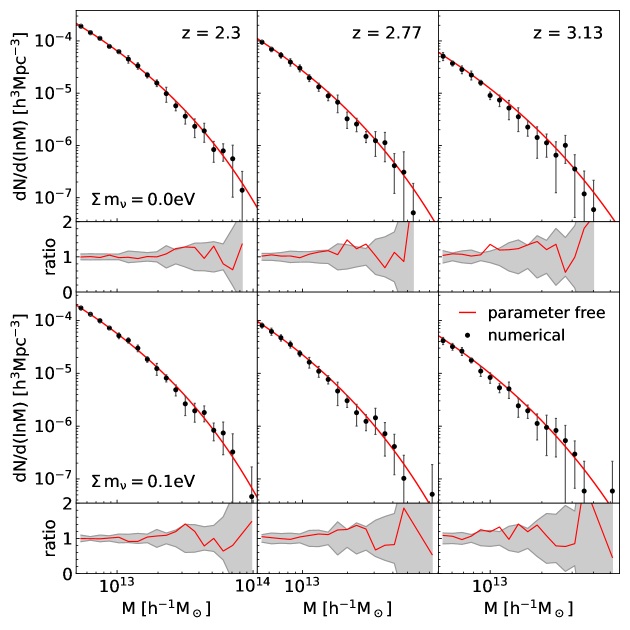
Figure 1 plots the numerically obtained splashback mass function (black closed circles) with the Jackknife errors at , and compares them with the analytic formula (red solid line) with the best-fit value of , for the two models in the first and third from the top panels. The ratios of the numerical result to the analytical formula for each model (red solid line) with one standard deviation scatter (gray area) are also shown in the third and first from the bottom panels. As can be seen, for both of the models, despite that it has only one parameter, the analytic formula excellently matches the numerical results in the wide mass range of at .
Repeating the same calculation but at higher redshifts, we trace . Figures 2-3 plot the same as Figure 1 but at and , respectively, demonstrating how well the analytic formula, Equations (1)-(3) with fixed , describes the splashback mass function even in the presence of neutrinos over a broad range of . Figure 4 shows how (black filled circles) changes with redshifts for the two cases of . As can be seen, for both of the cases, decreases almost linearly with redshifts at , showing a trend of converging to zero at some critical redshift, . If the diffusion coefficient vanishes, the analytic formula of the splashback mass function becomes parameter free. Figure 5 compares the numerical results at three edshifts beyond with the parameter-free model, Equation (4). Although the numerical results suffer from large Jackknife errors at these high redshifts due to the low number densities of massive cluster halos, the splashback mass functions agree quite well with the purely analytic model for both of the models at . These result are consistent with what Ryu & Lee (2021) found for the case of the CDM cosmology, confirming the validity of Equations (1)-(4) even in the presence of neutrinos.
As done in Ryu & Lee (2021), approximating in the range of to a linear fit, , we determine the best values of and via the standard -statistics, which are listed in Table 1 . As can be read, the two models differ in the best-fit values of and , the massive neutrino case yielding a substantially larger value of and significantly lower value of than the massless neutrino case. This result indicates that the presence of massive neutrinos has an effect of making more diffusive in this redshift range, slowing down the decrease of with . In other words, in the presence of hot DM particles like massive neutrinos that have large free streaming lengths, the DM halos experience larger amount of disturbance from the surrounding, which make it more ambiguous to precisely identify their physical boundaries.
Unlike the result of Ryu & Lee (2021) that linearly decreases with redshifts in the whole range from to , however, we find an anomalous behavior of at in the presence of neutrinos: it increases with , deviating from the linear fit at , as can be seen in Figure 4. We also note that the massive neutrino case exhibits a much more conspicuous deviation of from the linear fit than the massless case at these low redshifts. We suspect that it should be caused or at least linked closely with the inherent limitation of the SPARTA code in locating the splashback boundaries of DM halos at where the unknown future orbits of infalling particles make it impossible to determine particle apocenters (private communication with B. Diemer 2022).
4 Summary and Conclusion
We have numerically investigated the effect of neutrinos on the splashback mass functions of DM halos in the mass range of by applying the SPARTA code (Diemer, 2017) to the snapshots of MassiveNuS (Liu et al., 2018) for two different cosmologies with total neutrino mass of and . Comparing the numerically obtained splashback mass functions to the analytic single parameter formula proposed by Ryu & Lee (2021) at various redshifts, we have trailed the evolution of the single parameter, dubbed the diffusion coefficient , in the range of . It has turned out that the analytic formula with fixed splashback density threshold validly describes the splashback mass function for both of the models at redshifts up to and that the diffusion coefficient decreases almost linearly with redshifts at , evanescing at some critical redshift, which are all in consistent with the claim of Ryu & Lee (2021).
Fitting at to a linear scaling relation of for both of the models, we have determined the best-fit values of the slope, , and critical redshift, , and find that they sensitively depend on the total neutrino mass. The model with yields a significantly lower value of and a substantially higher value of than the other model with , which indicates that the diffusion coefficient decreases more slowly with in the presence of massive neutrinos. Since the diffusion coefficient of the analytic formula is a measure of the stochasticity of the splashback density threshold, this result implies that the presence of hot DM particles like massive neutrinos has an effect of disturbing more severely the splashback boundaries and making the halo identification more ambiguous. The dependence of and on also implies that the diffusion coefficient of the splashback mass function can in principle be used as a probe of the total neutrino mass.
A failure of the linear fit approximation to has been witnessed for both of the models at when the diffusion coefficient exhibit increment rather than decrement with , an anomalous tendency never detected in the absence of neutrinos for which case the linear fit always matches the diffusion coefficient in the entire range of . Given the fundamental limitation of the SPARTA code at that it is incapable of locating the apocenters of infalling DM particles whose future orbits are known (private communication with B. Diemer 2022), we suspect that the anomalous behavior of witnessed at should not be a real one caused by the presence of massive neutrinos but a spurious one caused by the inherent flaw of the SPARTA code at low redshifts.
It is, however, worth discussing a caveat that our conclusion is subject to. The MassiveNuS employed the analytic linear response approximation (Ali-Haïmoud & Bird, 2013) to mimic the presence of massive neutrinos rather than directly including the massive neutrinos as component particles. Although this approximation has been known to work quite well provided that (Bird et al., 2018), it is not guaranteed to accommodate all possible effects that the massive neutrinos would have on the nonlinear evolution of cosmic web. It will require a more rigorous and accurate treatment of the neutrino effects to investigate the true behavior in the nonlinear regime and its dependence on the total neutrino mass. It will be also quite desirable to have an analytic model for derived from the first principles, with which one can quantitatively probe the nature of dark matter including massive neutrinos. Our future work is in this direction.
References
- Adhikari et al. (2014) Adhikari, S., Dalal, N., & Chamberlain, R. T. 2014, JCAP, 2014, 019
- Ali-Haïmoud & Bird (2013) Ali-Haïmoud, Y. & Bird, S. 2013, MNRAS, 428, 3375
- Bond & Myers (1996) Bond, J. R., & Myers, S. T. 1996, ApJS, 103, 1
- Behroozi et al. (2013) Behroozi, P. S., Wechsler, R. H., & Wu, H.-Y. 2013, ApJ, 762, 109
- Bernardeau (1994) Bernardeau, F. 1994, ApJ, 427, 51
- Bertschinger (1985) Bertschinger, E. 1985, ApJS, 58, 39
- Bird et al. (2018) Bird, S., Ali-Haïmoud, Y., Feng, Y., et al. 2018, MNRAS, 481, 1486
- Bond et al. (1991) Bond, J. R., Cole, S., Efstathiou, G., et al. 1991, ApJ, 379, 440
- Bond et al. (1996) Bond, J. R., Kofman, L., & Pogosyan, D. 1996, Nature, 380, 603
- Borzyszkowski et al. (2017) Borzyszkowski, M., Porciani, C., Romano-Díaz, E., et al. 2017, MNRAS, 469, 594
- Chiueh & Lee (2001) Chiueh, T. & Lee, J. 2001, ApJ, 555, 83
- Corasaniti & Achitouv (2011a) Corasaniti, P. S. & Achitouv, I. 2011a, Phys. Rev. Lett., 106, 241302
- Corasaniti, & Achitouv (2011b) Corasaniti, P. S. & Achitouv, I. 2011b, Phys. Rev. D, 84, 023009
- Diemer et al. (2013) Diemer, B., More, S., & Kravtsov, A. V. 2013, ApJ, 766, 25
- Diemer & Kravtsov (2014) Diemer, B. & Kravtsov, A. V. 2014, ApJ, 789, 1
- Diemer & Kravtsov (2015) Diemer, B. & Kravtsov, A. V. 2015, ApJ, 799, 108
- Diemer (2017) Diemer, B. 2017, ApJS, 231, 5
- Diemer et al. (2017) Diemer, B., Mansfield, P., Kravtsov, A. V., et al. 2017, ApJ, 843, 140
- Diemer (2020a) Diemer, B. 2020a, ApJ, 903, 87
- Diemer (2020b) Diemer, B. 2020b, ApJS, 251, 17
- Diemer (2021) Diemer, B. 2021, ApJ, 909, 112
- Eke et al. (1996) Eke, V. R., Cole, S., & Frenk, C. S. 1996, MNRAS, 282, 263
- Fillmore & Goldreich (1984) Fillmore, J. A. & Goldreich, P. 1984, ApJ, 281, 1
- García et al. (2021) García, R., Rozo, E., Becker, M. R., et al. 2021, MNRAS, 505, 1195
- Gao & Theuns (2007) Gao, L. & Theuns, T. 2007, Science, 317, 1527. doi:10.1126/science.1146676
- Gunn & Gott (1972) Gunn, J. E. & Gott, J. R. 1972, ApJ, 176, 1
- Jenkins et al. (2001) Jenkins, A., Frenk, C. S., White, S. D. M., et al. 2001, MNRAS, 321, 372
- Komatsu et al. (2011) Komatsu, E., Smith, K. M., Dunkley, J., et al. 2011, ApJS, 192, 18
- Lahav et al. (1991) Lahav, O., Lilje, P. B., Primack, J. R., et al. 1991, MNRAS, 251, 128
- Lee (2019) Lee, J. 2019, ApJ, 872, L6
- Lesgourgues & Pastor (2012) Lesgourgues, J., & Pastor, S. 2012, Invited Review article for the Special Issue on Neutrino Physics, 608515; doi:10.1155/2012/608515
- Lesgourgues & Pastor (2014) Lesgourgues, J. & Pastor, S. 2014, New Journal of Physics, 16, 065002
- Lewis et al. (2000) Lewis, A., Challinor, A., & Lasenby, A. 2000, ApJ, 538, 473
- Liu et al. (2018) Liu, J., Bird, S., Zorrilla Matilla, J. M., et al. 2018, JCAP, 2018, 049
- Maggiore & Riotto (2010a) Maggiore, M., & Riotto, A. 2010a, ApJ, 711, 907
- Maggiore & Riotto (2010b) Maggiore, M., & Riotto, A. 2010b, ApJ, 717, 515
- More et al. (2015) More, S., Diemer, B., & Kravtsov, A. V. 2015, ApJ, 810, 36
- Pace et al. (2010) Pace, F., Waizmann, J. C., & Bartelmann, M. 2010, MNRAS, 1865, 1874
- Planck Collaboration et al. (2014) Planck Collaboration, Ade, P. A. R., Aghanim, N., et al. 2014, A&A, 571, A16
- Press & Schechter (1974) Press, W. H., & Schechter, P. 1974, ApJ, 187, 425
- Robertson et al. (2009) Robertson, B. E., Kravtsov, A. V., Tinker, J., et al. 2009, ApJ, 696, 636
- Ryu & Lee (2021) Ryu, S. & Lee, J. 2021, ApJ, 917, 98
- Shapiro et al. (1999) Shapiro, P. R., Iliev, I. T., & Raga, A. C. 1999, MNRAS, 307, 203
- Sheth & Tormen (1999) Sheth, R. K. & Tormen, G. 1999, MNRAS, 308, 119
- Sheth et al. (2001) Sheth, R. K., Mo, H. J., & Tormen, G. 2001, MNRAS, 323, 1
- Sheth & Tormen (2002) Sheth, R. K., & Tormen, G. 2002, MNRAS, 329, 61
- Tinker et al. (2008) Tinker, J., Kravtsov, A. V., Klypin, A., et al. 2008, ApJ, 688, 709
- Wang et al. (2009) Wang, H., Mo, H. J., & Jing, Y. P. 2009, MNRAS, 396, 2249
- Warren et al. (2006) Warren, M. S., Abazajian, K., Holz, D. E., et al. 2006, ApJ, 646, 881
- Wetzel et al. (2014) Wetzel, A. R., Tinker, J. L., Conroy, C., et al. 2014, MNRAS, 439, 2687