Further author information: (Send correspondence to J.N.A.)
J.N.A.: E-mail: [email protected]
The space coronagraph optical bench (SCoOB): 3. Mueller matrix polarimetry of a coronagraphic exit pupil
Abstract
High-contrast imaging in the next decade aims to image exoplanets at smaller angular separations and deeper contrasts than ever before. A problem that has recently garnered attention for telescopes equipped with high-contrast coronagraphs is polarization aberration arising from the optics. These aberrations manifest as low-order aberrations of different magnitudes for orthogonal polarization states and spread light into the dark hole of the coronagraph that cannot be fully corrected. The origin of polarization aberrations has been modeled at the telescope level. However, we don’t fully understand how polarization aberrations arise at the instrument level. To directly measure this effect, we construct a dual-rotating-retarder polarimeter around the SCoOB high-contrast imaging testbed to measure its Mueller matrix. With this matrix, we directly characterize the diattenuation, retardance, and depolarization of the instrument as a function of position in the exit pupil. We measure the polarization aberrations in the Lyot plane to understand how polarization couples into high-contrast imaging residuals.
keywords:
Mueller polarimetry, coronagraphy, polarization aberrations1 INTRODUCTION
Polarization aberrations are a known limiter to high-contrast imaging in the next decade. In advance of the Astro 2020 decadal survey, the LUVOIR and HabEx studies imposed constraints on the design of their OTA in order to minimize the presence of polarization aberrations that ultimately reach their coronagraphs[gaudi2020habitable, Will_polarization_luvoir]. The next-generation giant segmented mirror telescopes (GSMTs) experience considerable polarization aberration due to the large change in the angle of incidence in the telescope to fit within a reasonably-sized dome [anche2023polarization]. Much work has been done to model the polarization aberrations in astronomical telescopes; however, little is understood about the polarization aberrations at the instrument level.
To achieve contrast on a space-borne coronagraph, similar to the one on the future Habitable Worlds Observatory (HWO), the telescope will require unprecedented stability and performance. Quantifying all possible sources of error is necessary in order to achieve this target contrast. Inspired by the CDEEP mission concept[1], the Space Coronagraph Optical Bench (SCoOB )[2, 3, 4, Anche2024] is a vacuum-compatible coronagraph testbed at the University of Arizona’s Space Astrophysics Laboratory aimed at prototyping high-contrast imaging technology for space-based telescopes. SCoOB was designed to achieve high static contrast with relatively low polarization aberration[1], but the polarization aberrations of the coronagraph have never been evaluated. In this study, we construct a polarimeter around SCoOB to understand the presence of polarization aberrations at the coronagraph level.
Measurement of the polarization aberrations of a system requires an understanding of how it transforms the polarization state across a beam. Polarization aberrations are typically computed from the Jones pupil, which is a spatially varying Jones matrix at the exit pupil of an optical system. However, Jones matrices cannot be measured directly. In contrast, the Mueller pupil is a quantity that can be evaluated with a series of power measurements. This loses track of the global phase of the polarization aberration but enables an evaluation of how the polarization state is aberrated with respect to a reference phase. In this study, we seek to measure the Mueller pupil of SCoOB to gain an understanding of the degree of polarization aberration present in coronagraphic instruments. In Section 2, we outline the principle of a dual-rotating-retarder Mueller polarimeter (DRRP) that we use to measure the SCoOB Mueller matrix. In Section 3, we outline the assembly, calibration, and validation of the DRRP in the UA Space Astrophysics Laboratory. In Section 4, we show the results of placing the polarimeter around SCoOB to measure the Mueller pupil of the coronagraph. In Section 5 we evaluate what the results mean for calibrating SCoOB ’s static contrast floor, and outline a path for future investigation.
2 Dual-rotating Retarder Mueller Matrix Polarimetry
The DRRP is a commonly used device for measuring the Mueller matrix of an instrument. The DRRP was first described in Azzam 1978[5], where they describe the determination of a Mueller matrix by Fourier analysis of the detected signal from a device that modulates the polarization state sent to and observed from a unit under test. Smith 2002[6] describes the optimization of the free parameters of the DRRP for fast and precise measurement of the Mueller matrix. Chapter 7 of Chipman, Lam, and Young[7] describes a variation on the data reduction for a DRRP that is computationally simple to implement, which we reproduce in this section.
The Mueller matrices for a linear polarizer () and linear retarder () are given by Equations 1 and 2.
| (1) |
| (2) |
A DRRP can be characterized by a sequence of a source, polarization state generator (, given by Equation 3), a sample to measure, and a polarization state analyzer (, given by Equation 4). A diagram of the DRRP is shown in Figure 1.
| (3) |
| (4) |
The DRRP measures the Mueller matrix of a sample through a series of measurements where the retarders are progressively rotated. In this study, for every that the polarization state generator waveplate is stepped, the polarization state analyzer is stepped by . However, Smith[6] notes that other angular velocity ratios may be more optimal for rapid polarimetry.

Using a Mueller matrix model of the polarimeter, we construct a polarimetric data reduction matrix that is given by Equation 5,
| (5) |
where is the Kronecker product, and are the first row and column vectors of the and , respectively. The Mueller matrix is computed using the pseudo-inverse of , , multiplied by the vector of observed power , as shown in Equation 6,
| (6) |
where the result is a vector that contains the Mueller matrix.
3 Assembly and Operation of a Dual Rotating-Retarder Mueller Polarimeter
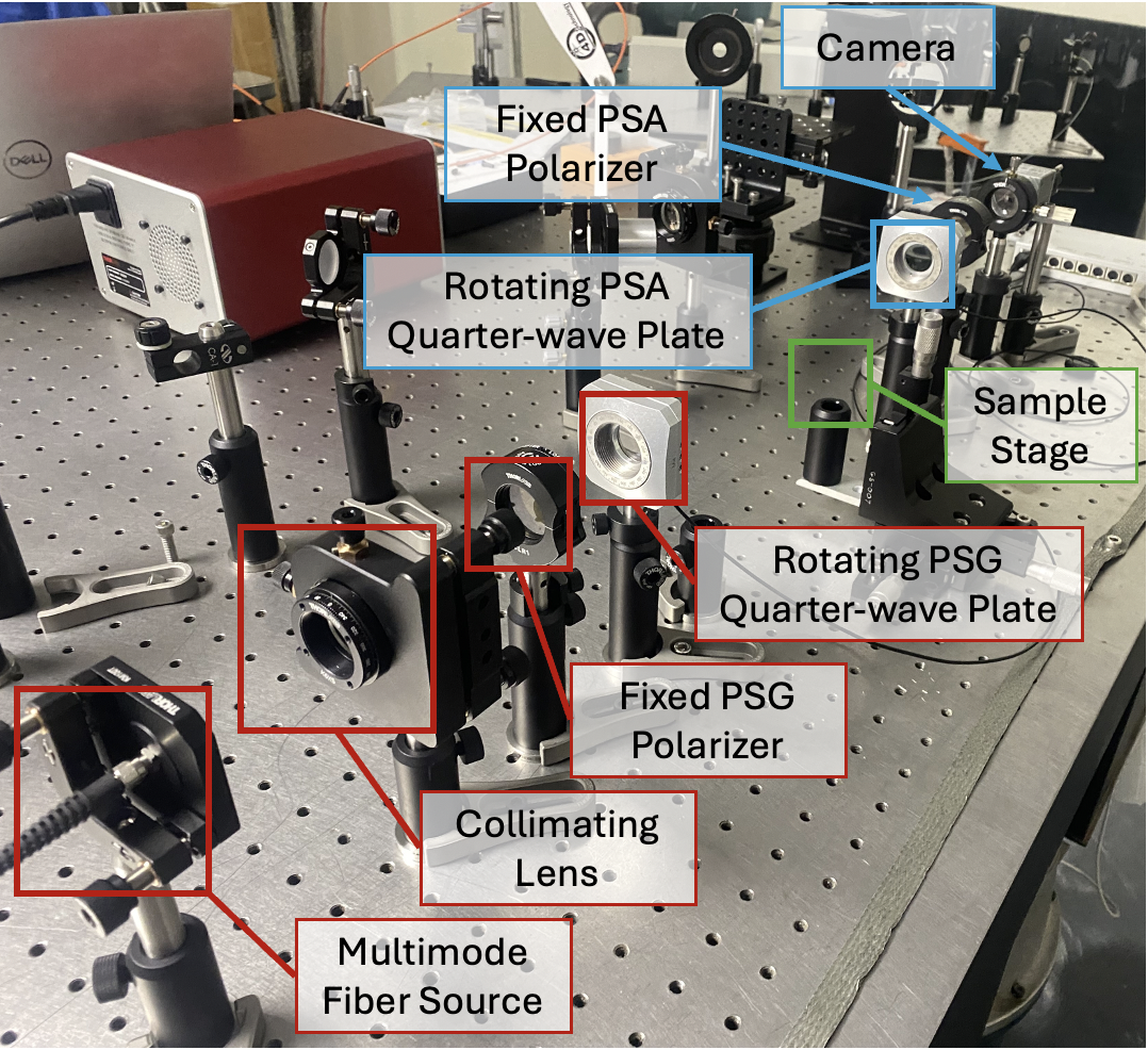
We construct the DRRP facility in the UA Space Astrophysics Laboratory (UASAL) using entirely commercial off-the-shelf components, a list of which is included in the appendix of this manuscript. Figure 2 shows the DRRP assembled in the clean tent in UASAL. We use the Newport Agilis Piezo Motor Driven Rotation Stages with the AG-UC8 controller to rotate the quarter-wave retarders used in the DRRP. These rotation stages are driven via serial communication and lack encoders that indicate their current angular position, so we must calibrate the step sizes of the stages. To provide an open-source platform for serial communication of these rotation stages, we have created the katsu Python package[Ashcraft_Katsu]. katsu utilizes the Pyserial Python package for serial communication with a more user-friendly API than the standard command string interface supplied by Newport111https://www.newport.com/mam/celum/celum_assets/np/resources/Agilis_Piezo_Motor_Driven_Components_User_Manual.pdf?1, and also contains routines for Mueller matrix modeling, polarimetric data reduction, and Mueller matrix analysis. We use katsu for the entirety of the investigations contained in this proceedings.
3.1 Polarimeter Calibration
The goal of Mueller polarimeter calibration is to determine the most accurate polarimetric data reduction matrix as possible. To begin the calibration, we first perform an air measurement. We know the Mueller matrix of air to be nearly an identity matrix, which constrains the state of our system. The Mueller matrix of the polarimeter for a given state is then given by Equation 7,
| (7) |
The or top-left element of this matrix corresponds to the power measured as a function of the six free parameters. In practice, by alignment of the polarimeter we can get close to understanding the rotation angles of the system. We should also have some idea of the diattenuation of the polarizers and retardance of the retarders based on the manufacturer’s specifications. We use the Newport Agilis series rotation mounts, whose angular steps are unknown. Therefore we also calibrate the angular steps of the mounts in the air measurement. We curve fit to the observed power at the detector plane using the scipy.optimize.minimize function with the BFGS optimizer method. The results using 24 measurements are shown in Figure 3.

| Parameter | Guess Value | Calibrated Value |
|---|---|---|
Fitting the free parameters of our polarimeter to the measured data enables a more accurate understanding of the instrument state, which in turn enables a more accurate polarimetric data reduction matrix. Repeating the same number of measurements with an updated understanding of the instrument state enables a Mueller matrix measurement, which we show in Figure 4 for the case of a simple air (left) and vertical linear polarizer (right) measurement.

4 Results
To measure the SCoOB Mueller Pupil, we disassemble the polarimeter built in the UASAL laboratory and re-construct it in the TVAC chamber. We then perform an air calibration in the TVAC chamber to calibrate the state of the polarimeter before placing the PSA in the Lyot plane of the coronagraph without the coronagraph mask in, as shown in Figure 5. Here a SuperK tunable laser is used for the source instead of the halogen lamp used for the results in Figure 4. For both the calibration and the measurement of the Mueller Pupil, we take 40 measurements in angular increments of approximately for the PSG waveplate and for the PSA waveplate. We take two measurements, one at 630nm and another at 525nm, to understand how the polarization properties change as a function of wavelength. The results for are shown in Figure 6.


While it is useful to consider the full Mueller pupil of SCoOB , in order to translate this into a diffraction model, we must separate depolarization from the Mueller pupil. Lu and Chipman famously derived an interpretation of Mueller matrices based on the polar decomposition. In this expression, the Mueller matrix can be considered a multiplication of a depolarizer, retarder, and diattenuator [Lu:96], as shown in Equation 8,
| (8) |
Here is the depolarizer, is the retarder, and is the diattenuator. The decomposition method is shown in Lu and Chipman[Lu:96], but we built the algorithm into the Katsu Python package for broader use. Applying the polar decomposition to the Mueller pupil in Figure 6 yields the data in Figures 7 - 9. From these data, we can plot the total diattenuation, retardance, and depolarization of the system. The diattenuation () is given by Equation 9,
| (9) |
The retardance () is given by Equation 10,
| (10) |
And the depolarization index () is given by Equation 11,
| (11) |
The polar-decomposed Diattenuator, Retarder, and Depolarizer of the measured Mueller pupil in Figure 6 are given in Figures 7-9. Computing the polarization aberration quantities in Equations 9-11 for the Mueller pupil enables us to view the polarization aberrations of the system across the exit pupil of the coronagraph, which we show in Figure 10. There is a diattenuation across the pupil of approximately with a standard deviation of . Furthermore, we observe nonuniform behavior in the retardance plot that has a standard deviation of approximately radians, or . The depolarization index across the pupil is very near 1, indicating a lack of depolarization in the system. The standard deviation of these data is , but much of that signal is dominated by artifacts from the dust diffraction, so the depolarization of the coronagraph should be less than that.


The mid-frequency structure that is apparent in Figures 6 - 10 is perhaps the most interesting result of this study. They are of a higher spatial order than is predicted by typical polarization ray traces of simple systems (tilt/focus-like shapes), and consequently, their origin is unknown. Note that these patterns are not present in the laboratory measurements of air and a linear polarizer in Figure 4. Most likely, we are observing the influence of imperfect coatings on the polarized exit pupil of the coronagraph. Understanding how these effects translate to the minimum achievable contrast of the coronagraph will be critical to assessing how sensitive coronagraphs are to coating nonuniformity.
For a preliminary analysis into the impact of the as-measured polarization aberrations on SCoOB ’s contrast floor, we can convert the non-depolarizing Mueller pupil into a Jones pupil and propagate it through a charge-6 vector vortex coronagraph using HCIPy[por2018hcipy]. The computation of the Jones pupil is illustrated by Equation 12,
| (12) |
Where the amplitudes are given by Equations 13-16, and the relative phases are given by Equations 17-19. Note that while the amplitudes are completely determined, the phases must be determined relative to some reference because global phase is lost when measuring intensity. The Jones matrix and corresponding focal plane after propagation through a charge-6 vector vortex coronagraph with an diameter Lyot stop is shown in Figure 11. The as-measured polarization aberrations appear to result in a degradation of the normalized intensity from , but as shown in Van Gorkom et al (these proceedings)[4], after the application of focal plane wavefront sensing and control, SCoOB is capable of reaching contrasts of . Therefore, we know that these polarized wavefront errors are not fundamentally limiting at these locations on the focal plane. In future work we will assess the influence of these as-measured polarization aberrations on a simulated SCoOB dark hole in the presence of wavefront sensing and control.
| (13) |
| (14) |
| (15) |
| (16) |
| (17) |
| (18) |
| (19) |

5 Discussion
This study introduces the dual-rotating-retarder Mueller polarimeter as a characterization methodology for assessing the polarized performance of coronagraphic optical systems. We built our methods and data reduction into an open-source Python package called katsu, which is freely available on GitHub. Using katsu, we illustrate the principle of dual-rotating-retarder Mueller polarimetry in the lab for simple optical element characterization and then apply it to the polarimetry of the SCoOB testbed. We find a nominal diattenuation of , and a retardance standard deviation of , with little depolarization. We also observe a clear mid-frequency (4-5 cycles/pupil) structure in each of the elements of the Mueller pupil and corresponding polarization aberration pupils in Figure 10. Understanding the influence of this aberration will be the subject of future work to calibrate the static contrast floor of SCoOB .
Understanding the origin of the mid-frequency aberration revealed in this study is a key next step for this work. However, characterizing film uniformity across an aperture is a non-trivial task. In principle, this could be achieved through ellipsometry. By depositing the same mirror coating used for the SCoOB mirrors on a flat substrate, the ellipsometric characteristics can be studied at multiple points across the substrate. These data can be fit to a layer model that includes a refractive index tensor to more precisely understand the degree of birefringence in the system.
Acknowledgements.
This work was supported by a NASA Space Technology Graduate Research Opportunity. The research presented in these proceedings was predominantly conducted with open-source software, including: Poke[Ashcraft_2023], Katsu[Ashcraft_Katsu], HCIPy[por2018hcipy], numpy[harris2020array], scipy[2020SciPy-NMeth], matplotlib[Hunter:2007], and IPython[PER-GRA:2007].6 Appendix:


| Vendor | Part |
|---|---|
| Thorlabs | Stabilized Tungsten-Halogen Light Source SLS201L |
| NKT Photonics | SuperK COMPACT white light laser |
| Newport | Agilis PR100-V6 |
| Newport | Agilis AG-UC8 Controller |
| Meadowlark | High-contrast Linear Polarizer |
| BVO | Quarter-wave Plate |
References
- [1] Maier, E. R., Douglas, E. S., Kim, D. W., Su, K., Ashcraft, J. N., Breckinridge, J. B., Choi, H., Choquet, E., Connors, T. E., Durney, O., Gonzales, K. L., Guthery, C. E., Haughwout, C. A., Heath, J. C., Hyatt, J., Lumbres, J., Males, J. R., Matthews, E. C., Milani, K., Montoya, O. M., N’Diaye, M., Noenickx, J., Pogorelyuk, L., Ruane, G., Schneider, G., Smith, G. A., and Stark, C. C., “Design of the vacuum high contrast imaging testbed for CDEEP, the Coronagraphic Debris and Exoplanet Exploring Pioneer,” in [Space Telescopes and Instrumentation 2020: Optical, Infrared, and Millimeter Wave ], Lystrup, M., Perrin, M. D., Batalha, N., Siegler, N., and Tong, E. C., eds., 11443, 114431Y, International Society for Optics and Photonics, SPIE (2020).
- [2] Ashcraft, J. N., Choi, H., Douglas, E. S., Derby, K., Gorkom, K. V., Kim, D., Anche, R., Carter, A., Durney, O., Haffert, S., Harrison, L., Kautz, M., Lumbres, J., Males, J. R., Milani, K., Montoya, O. M., and Smith, G. A., “The space coronagraph optical bench (SCoOB): 1. Design and assembly of a vacuum-compatible coronagraph testbed for spaceborne high-contrast imaging technology,” in [Space Telescopes and Instrumentation 2022: Optical, Infrared, and Millimeter Wave ], Coyle, L. E., Matsuura, S., and Perrin, M. D., eds., 12180, 121805L, International Society for Optics and Photonics, SPIE (2022).
- [3] Gorkom, K. V., Douglas, E. S., Ashcraft, J. N., Haffert, S., Kim, D., Choi, H., Anche, R. M., Males, J. R., Milani, K., Derby, K., Harrison, L., and Durney, O., “The space coronagraph optical bench (SCoOB): 2. Wavefront sensing and control in a vacuum-compatible coronagraph testbed for spaceborne high-contrast imaging technology,” in [Space Telescopes and Instrumentation 2022: Optical, Infrared, and Millimeter Wave ], Coyle, L. E., Matsuura, S., and Perrin, M. D., eds., 12180, 121805M, International Society for Optics and Photonics, SPIE (2022).
- [4] Gorkom, K. V., Douglas, E. S., and Ashcraft, J. N., “The space coronagraph optical bench (scoob): 4. vacuum performance of a high contrast imaging testbed,” in [Space Telescopes and Instrumentation 2024: Optical, Infrared, and Millimeter Wave (These Proceedings) ], International Society for Optics and Photonics, SPIE (2024).
- [5] Azzam, R. M. A., “Photopolarimetric measurement of the mueller matrix by fourier analysis of a single detected signal,” Opt. Lett. 2, 148–150 (Jun 1978).
- [6] Smith, M. H., “Optimization of a dual-rotating-retarder mueller matrix polarimeter,” Appl. Opt. 41, 2488–2493 (May 2002).
- [7] Chipman, R. A., Lam, W.-S. T., and Young, G., [Polarized Light and Optical Systems ], CRC Press (2018).