The Southern Hemisphere Narrow-Line Seyfert 1 Infrared Survey
Abstract
We present a near-infrared spectroscopic survey of narrow-line Seyfert 1 galaxies in the southern hemisphere (using the SOFI instrument on the ESO-NTT telescope), sampled from optical surveys. We examine the kinematics of the broad-line region, probed by the emission line width of hydrogen (Pa and H ). We observed 57 objects, of which we could firmly measure Pa in 49 cases. We find that a single Lorentzian fit (preferred on theoretical grounds) is preferred over multi-component Gaussian fits to the line profiles; a lack of narrow-line region emission, overwhelmed by the pole-on view of the broad line region (BLR) light, supports this. We recompute the catalog black hole (BH) mass estimates, using the values of FWHM and luminosity of H , both from catalog values and re-fitted Lorentzian values. We find a relationship slope greater than unity compared to the catalog values. We ascribe this to contamination by galactic light or difficulties with line flux measurements. However, the comparison of masses computed by the fitted Lorentzian and Gaussian measurements show a slope close to unity. Comparing the BH masses estimated from both Pa and H , the line widths and fluxes shows deviations from expected; in general, however, the computed BH masses are comparable. We posit a scenario where an intermixture of dusty and dust-free clouds (or alternately a structured atmosphere) differentially absorbs the line radiation of the BLR, due to dust absorption and hydrogen bound-free absorption.
keywords:
galaxies: active – galaxies: Seyfert Unified Astronomy Thesaurus concepts: Seyfert galaxies (1447), Active galactic nuclei (16), Supermassive black holes (1663), Near infrared astronomy (1093), Spectroscopy (1558)1 Introduction
Narrow-line Seyfert 1 (NLSy1) galaxies are a class of active galactic nuclei (AGN) where the broad-line region (BLR) H emission lines show characteristic velocities full-width half-maximum (FWHM) 2000 km s-1 and flux ratio of [O iii]/H 3, as well as prominent Fe II lines (Osterbrock & Pogge, 1985; Goodrich, 1989). These characteristics can be interpreted as either (a) a relatively under-massive black hole (BH) typically 106-8 M⊙(vs. 107-9 M⊙ for typical broad-line Seyfert 1s), with correspondingly high Eddington ratio/accretion rate (0.1 to 1), suggesting a young, fast-growing phase of the AGN (Viswanath et al., 2019; Berton et al., 2015), or (b) the BLR is disk-like and viewed pole on; thus Doppler broadening is suppressed and the apparent low mass of the BH is merely an inclination effect (Jolley & Kuncic, 2008). The BLR models of Goad et al. (2012), which have a bowl-shaped geometry combined with turbulence, naturally favour the second view.
Radio-loud NLSy1 galaxies (only about 7% of all NLSy1 galaxies) share some of the characteristics of blazars, including -ray emission (Abdo et al., 2009) and radio beamed jets (Foschini et al., 2015), albeit at lower luminosity and BH mass. The similarity to blazars suggest a pole-on orientation (Decarli et al., 2008, 2011); this corrects for the lower BH masses and high Eddington ratios, which are then more in line with their host galaxy scaling relationships, e.g. (e.g. Ryan et al., 2007).
We present results from an infrared spectroscopic survey of this class of objects. Our primary objective is to study the kinematics of the gas in the line emitting region, which are probed by the Pa and H emission lines. Observations in the near infra-red (NIR) have the advantage of penetrating obscuring dust; the Pa emission line flux (1875 nm) is less affected than the H flux (486.3 nm) and thus sees “deeper”.
The mass of the BH can be estimated from the luminosity and full-width half-maximum (FWHM) velocity of the broad hydrogen emission lines from the BLR (see e.g. Kim et al., 2010; Popović, 2020, and references therein). We will compare methods of estimating this mass with different emission lines, line profile models and continuum parameters.
This paper is organized as follows. In Section 2, we present the sample selection; in Section 3, we discuss the observations, data reduction and emission-line measurement methods and results and in Section 4, we estimating the black hole masses by the different methods (including comparison with optical emission lines) and calculate the extinctions in the BLR. In Section 5, we discuss our results, and in Section 6, we present our conclusions.
For consistency with the source surveys for our sample, we adopt the cosmological parameters km s-1, and .
2 Sample Selection
Our selection of galaxies are from two previous surveys. Chen et al. (2018)111http://cdsarc.u-strasbg.fr/viz-bin/qcat?J/A+A/615/A167 (hereafter C18) classified 167 southern hemisphere galaxies as NLSy1s from the Six-degree Field Galaxy Survey (6dFGS) final data release (DR3) (Jones et al., 2004, 2009)222http://www-wfau.roe.ac.uk/6dFGS/; they derived flux-calibrated spectra and found strong correlations between the monochromatic luminosity at 5100Å and the luminosities of H and [O iii] lines, with typical SMBH masses (106–108 M⊙) and high Eddington ratios (a median of 0.96) for the AGN class. The survey of Schmidt et al. (2018)333http://cdsarc.u-strasbg.fr/viz-bin/qcat?J/A+A/615/A13 (hereafter S18) (28 galaxies) was focused on [O iii] line profile asymmetries associated with outflows, confirming the correlation between the blueshift and FWHM of the line core, between the outflow velocity and the black hole mass and with the width of the broad component of H . Removing objects common to the two catalogs gave a target list of 189 galaxies with declination . The redshifts () are in the range (which corresponds to a luminosity distance range of 44 to 2855 Mpc).
Hydrogen emission line flux can come from both AGN activity and star formation (SF). To determine whether SF is significant in our sample, we use mid infrared (MIR) color-color plots from WISE satellite data. We retrieved the WISE magnitudes from the AllWISE catalog (Wright et al., 2010); Figure 1 (left panel) shows the W2-W3 vs. W1-W2 plot (overlaying the color-color diagram from Wright et al., 2010, their Figure 12), with point colors indicating the object redshift. Most galaxies are in the Seyfert/QSO locus, with some having an admixture of stellar light. None are within the starburst (SF) region, which indicates minimal, if any, star formation in our sample. The single point near (0.5,0) is due to sky contamination by galactic cirrus. We note that the plot exhibits a trend with redshift; this is expected as the spectral peak of the warm dust (with maximum in the W2 band) is red-shifted, effectively a K-correction. Figure 2 shows the trend of colors with redshift. In a similar manner, we also plotted the 2MASS JHK color-color diagram (Figure 1 - right panel); this also shows a trend with redshift as per the WISE diagram.
We also test the reliability of WISE color selection on our sample; we use the 90% reliability criterion (R90) from Assef et al. (2018), finding that our objects are selected as AGN at this reliability in 93.5% (177/189) of cases. Those that are rejected have a redshift population significantly less than those accepted; the Student’s one-tailed t-test on the redshifts shows a p-value of , i.e. we can reject the hypothesis that the populations are the same (rejected - N=12, ; selected - N=177, ). This is most likely due to contamination by galactic stellar light.


3 Methods
3.1 Observations and Data Reduction
We observed a sub-sample of these galaxies with the SofI (Son of ISAAC) near infrared (NIR) spectrometer (Moorwood et al., 1998) at the Nasmyth A focus of the ESO 3.5-m New Technology Telescope (NTT) at the European Southern Observatory (ESO) in La Silla (Chile), in the program 0103.B-0504(B) (observation dates 25–27 August 2019). To maximize efficiency, our observing strategy was to prioritize objects based on a figure of merit, which selected both on 2MASS Ks magnitude (Skrutskie et al., 2006, with sample range of 10.9–17.4 mag) and on total H flux (from erg s-1) as taken from the C18 and S18 catalogs, i.e. we selected both bright galaxies and strong emission lines.
The GRF (red) grism was used with a 1″ slit width, for a spectral range of 1495-2518 nm and a spectral resolution . For the redshift range, this allows for observation of at least one hydrogen line (Pa , Br or Pa ) plus [Fe ii] (all objects) or [Fe ii] (56/189) plus H2 (133/189). The Pa emission line falls within the atmospheric absorption band ( nm) in 12 of 171 objects where the line was within the spectral range of the instrument, but even then the Pa line is strong enough to be measured in some of these cases.
Over the three nights, 55 objects were successfully observed in the standard ABBA spectroscopic mode (the observing template ”SOFI_spec_obs_AutoNodOnSlit”), using jitter between each AB pair to reduce the effect of bad pixels. Each exposure was 150 sec for a cycle total of 10 min. Fainter objects were observed with 2 ABBA cycles.
For each galaxy, an A0 star at a similar airmass was also observed as a telluric standard and flux calibrator with a single AB pair, each frame of 10 sec exposure. Some galaxies shared the same standard star, as they were close together on sky.
The data were reduced in the standard manner using the gasgano444http://www.eso.org/sci/software/gasgano.html software with the “sofi_spc_jitter” recipe, with flat-fielding and wavelength calibration. Telluric correction and flux calibration were performed using an A0V stellar spectral template (from the ESO stellar library of Pickles, 1998). The spectra were re-dispersed to the range 1495-2518 nm, with 1 nm steps. The velocity resolution is 200 km s-1. The spectra were corrected for galactic extinction, using data from the IRSA Galactic Dust Reddening and Extinction service555https://irsa.ipac.caltech.edu/applications/DUST/ using the Schlafly & Finkbeiner (2011) values and the Cardelli et al. (1989) extinction law. Galactic extinction for the catalog objects is in the range 0.007–0.58. They were then wavelength shifted to restframe and cleaned (specifically, blanking the region between the H and K atmospheric windows and also removing single-pixel noise).
One object from the catalogs (WPV85007 = HE0036-5133) had already been observed with SOFI by Busch et al. (2016)666http://cdsarc.u-strasbg.fr/viz-bin/qcat?J/A+A/587/A138 using the same telescope setup; we incorporated the spectrum into our sample. Another object, 6dF-J070841.5-493306 (1H0707-495) had been observed with SINFONI on the VLT, with the data being retrieved from the ESO archive (program ID 092.B-0279(B), PI A.C. Fabian). After standard data reduction using gasgano, we used an aperture of 1.75″ on the resulting data cube to extract the galaxy spectrum. This aperture was determined by a curve-of-growth measurement using increasing aperture sizes.
Table 3 list a sample of the objects with coordinates, redshift, luminosity distance, galactic extinction and K magnitude, plus observation details. The complete table is available online and as supplementary material, as described below.
The pipeline does not give a noise spectrum directly; we can estimate (at least for comparative purposes) a signal-to-noise ratio from the spectrum itself by measuring the average and standard deviation over a spectral window in a “quiet” region (i.e. free of atmospheric absorption and spectral features). In general, we use a wavelength of 2000 nm with a window of 100 nm. The resulting values are also given in Table 3, and range from 5–75.
3.2 Sampling Bias
We would expect our observations to be a somewhat biased sub-sample of the source catalogs, since the observational priority was given to K-band bright objects with strong H fluxes. Figure 3 show the histograms of the observed vs. catalog distributions of redshift, W1, K magnitude and H log luminosity; the observed objects are somewhat brighter in magnitude and closer then the complete sample; the H luminosity is somewhat better sampled.

3.3 Emission Line Fitting - Gaussian vs. Lorentzian Profiles
Emission lines profiles are typically de-blended into several Gaussian components, which are then equated to individual gas masses with separate kinematics. Both C18 and S18 use multiple Gaussian fits to the observed line profiles, as do other surveys (e.g. Dopita et al., 2015, the S7 survey). These fits assume that the narrowest component(s) represents the narrow-line region (NLR) emission, with a single broad component being the BLR emission. However, a Lorentzian fit for the BLR emission (especially for NLSy1’s) is more physically motivated, both on observational (Kollatschny & Zetzl, 2013; Berton et al., 2020) and theoretical grounds (Goad et al., 2012), whose models posit a bowl-shaped BLR bounded by a toroidal obscuring region.In their models, the presence of low inclination and significant turbulence leads to narrow cores and extended broad wings in the line profiles. Similar models have been proposed by Gaskell et al. (2007) and Gaskell (2017).
As a Lorentzian fit is very similar to a 2-component Gaussian fit, this may lead to a spuriously high value for the NLR emission component. Berton et al. (2020) concludes that the line shape (either Gaussian or Lorentzian) reveals two populations with different black hole masses, Eddington ratios and [O iii] and Fe II strengths. However, for our purposes, we can use a single Lorentzian fit, since we are comparing two emission lines from each object and the estimates of M∙ will not be affected greatly by the specific line shape.
We used the QFitsView777http://www.mpe.mpg.de/~ott/dpuser/qfitsview.html (Ott, 2012) de-blending functionality to fit all emission lines; this allows for both Gaussian and Lorentzian fits with multiple components. This requires some manual input from the user to set the initial estimates of continuum, height, centre and width and uses the GSL888https://www.gnu.org/software/gsl/doc/html/index.html “gsl_multifit” routines, returning fit values and errors of each component (continuum slope, central wavelength, FWHM and flux).
As an example, we fit a single Lorentzian function vs. 2 Gaussians (1 broad + 1 narrow) to the Pa spectral line of 6dF J202557.4-482226 (= 2MASS J20255738-4822261, z=0.06707). These fits are plotted in Figure 4; the residuals are plotted as standard deviations, i.e. the value is divided by the estimated spectral noise (in this case erg cm-2 s-1). The residuals from the two fits are of the same size; Occam’s razor leads us to prefer the Lorentzian fit (apart from the physical motivation described above). Comparing the fluxes, the Lorentzian fit flux is erg cm-2 s-1, whereas the combined Gaussian broad and narrow fit flux is erg cm-2 s-1, so M∙ will be underestimated if just the broad Gaussian component is used. The dispersion (second moment) of a Lorentzian curve is just the FWHM, whereas for a Gaussian curve =FWHM/2.355.
Several authors (Brotherton et al., 1994; Crenshaw & Kraemer, 2007; Dopita et al., 2015; Schmidt et al., 2016; Spence et al., 2018) fit an intermediate velocity component in the BLR emission lines, as well as the standard broad component. Our data show no requirement for this component with Lorentzian fits. On this basis, we will fit the hydrogen broad lines with a single Lorentzian curve.

Of the 57 objects in the NIR sample, we could firmly measure Pa in 49 cases. One object (6dF J195705.3-414117) had Pa visible, as the redshift of 0.374 moved Pa out of the measurement wavelength range. In this case, the measured Pa flux was multiplied by 2.07 (the canonical ratio) to estimate the Pa flux. Two object had poor noise levels and the remaining 5 objects had the Pa wavelength in the atmospheric absorption gap between the H and J bands. We could measure one object with Pa in this band, and the line was strong enough to dominate over the noise.
A sample of the flux and FWHM measurement results are given in Table 4 with the derived luminosity, velocity dispersion and black hole mass estimates; these are calculated as discussed in Section 4. The uncertainties in the flux and FWHM values are 1 errors from the fitting routines in QFitsView. The luminosity distance is computed from the redshift using the functionality implemented in TOPCAT999http://www.star.bristol.ac.uk/~mbt/topcat/ (Taylor, 2005), which depends on the cosmological parameters given above. The velocity dispersions have been corrected for instrumental resolution (6dF (C18) , REOSC (S18) , SOFI ) and the flux values are in units of 10-15 erg cm-2 s-1. The complete table is available online and as supplementary material, as described below.
3.4 Flux Calibration of Optical Spectra
As we wish to measure the hydrogen lines in the optical regime to compare black hole mass calculations and examine extinction in the BLR, we must ensure that the optical flux calibration is accurate. The S18 catalog provided flux-calibrated spectra, but C18 used spectra from the 6dFGS survey, which are not flux-calibrated in their raw form. C18 devised a calibration procedure by comparing the 6dFGS spectra with Sloan Digital Sky Survey (SDSS) spectra of the same object; they calculated the ratio of the 6dFGS over SDSS spectra for 7 radio-quiet (therefore minimally variable) cross-matched objects and fitted the averaged spectra with a fifth-order polynomial curve, which was used to calibrate all the spectra. We performed this analysis and obtained the same result. The spectra were then adjusted for galactic extinction as described above, and shifted to restframe. The S18 spectra were also extinction-corrected (they had been shifted to restframe before publication).
As a cross-check, we compared the flux-calibrated 6dFGS spectra from C18 with the 6 cross-matched S18 spectra. In general, the match for the spectral shape was excellent, however the flux ratios were somewhat scattered over a range of 1/3 to 3, with an average ratio of 1.2. A factor of 2 error in the flux values leads to a difference of 0.25 dex in M∙.
When comparing spectra in different wavelength bands and instruments, the major systematic differences are flux calibrations and aperture effects. The SOFI observations used a 1″ slit, whereas the 6dF science fibres have an aperture of 6″.7. It would be possible to constrain the optical flux calibration by requiring that the optical and NIR spectra be smoothly continuous, but the uncertainties from aperture effects preclude this. We consider that the apertures are large enough to accommodate the (presumably) point-source BLR, and thus to capture the whole emission-line radiation.
4 Results
4.1 Black Hole Mass Estimation
4.1.1 Mass Estimate by vs. H Luminosity
In general, M∙ is estimated from a relationship which assumes virialised gas clouds in the BLR:
| (1) |
where is the radius of the BLR, is the gas velocity, is the gravitational constant and is a factor dependant on the BLR geometry. The FWHM of the H line is a proxy for the rotational velocity of the gas, and the luminosity of the continuum at 5100 Å () is a proxy for the , proportional to . Greene & Ho (2005) also showed that H (and thus H ) broad line emission has a tight relationship with .
C18 based their estimation of M∙ of their catalog objects on the continuum luminosity and the dispersion of the H broad line (Foschini et al., 2015; Bentz et al., 2013; Berton et al., 2015). S18 used the methods of Greene & Ho (2005) (i.e. based mainly on the H line attributes, their Eqns. 6 and 7); of the 28 galaxies in the catalog, 26 use the H line and 2 use the H line. Kim et al. (2010) derived black hole mass estimates from Pa lines, comparing with those derived from either reverberation mapping method or single-epoch measurement method using Balmer lines. For consistency, we will use the relationships from Kim et al. (2010).
The relationship for M∙ with emission line parameters is:
| (2) |
where and are the luminosity and FWHM of species (Pa or H ), and the constants are given in Table 1; we follow the recommendation of Kim et al. (2010) to use the relationship which has the more physical exponent of the FWHM fixed at . We note that the value of is very close to the theoretical value of 0.5.
| Pa | 2 | ||
|---|---|---|---|
| H | 2 |
As an example, we show a plot of the optical and infrared spectra of the object 6dF J2025574-482226, with the Lorentz fits on both the H and Pa lines (Figure 5). Figure 6 shows the fits compared in greater detail where the continuum is removed and the wavelength is converted to relative velocity. As can be seen, the Pa spectral line is somewhat narrower than the H line; this will be discussed below. A complete set of plots of the line fits for all the 48 objects with both Pa and H flux is available online as as supplementary material.


4.1.2 Recalculated Mass from Optical Measurements
We re-measured the H broad line with a single Lorentzian curve for all objects that had measurable Pa flux in our survey (see Section 3.1) using the QFitsView functionality, and recomputed M∙ with the measured flux and FWHM. The line widths were corrected for instrumental dispersion. We compared the catalog data with the flux, luminosity and FWHM values derived from the Lorentzian fit; Figure 7 shows this. On these plots, the diagonal lines denote the equality between the measures; while the broad component fluxes and luminosities are very similar, the FWHM measurements are somewhat more scattered. This is more prevalent in the S18 data; this is probably due to (1) measuring H instead of H , and (2) the difficulty of de-composing the H from the associated [N ii] lines.


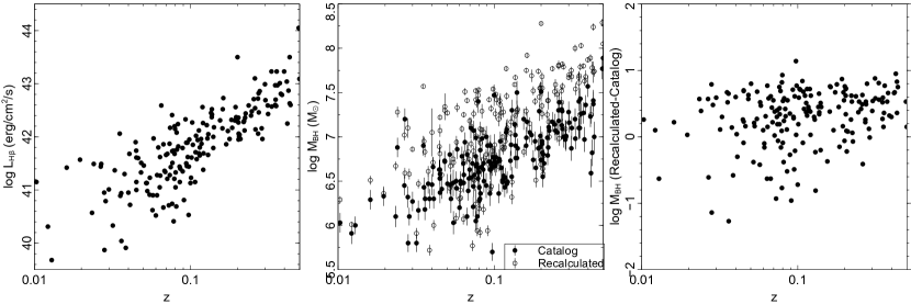
Using the catalog values of H flux and FWHM, we can re-derive the M∙ using the method given in Kim et al. (2010) and compare that with the M∙ of the original catalogs (Figure 8 - left panel).
We performed an orthogonal least squares regression analysis using the BCES method of Akritas & Bershady (1996)101010The BCES routine was from the Python module written by Rodrigo Nemmen (Nemmen et al., 2012), which is available at https://github.com/rsnemmen/BCES; this regression method is preferred because there is no independent variable and both data sets have errors. The best-fit slope for the catalog vs. recalculated M∙ (Figure 8 - left panel in black) is:
| (3) |
We note that the S18 masses are more scattered and somewhat below the fit line; this is probably due to the difficulties of measuring the H FWHM, as discussed before. If we fit just the C18 data, the fit is (Figure 8 - left panel in red):
| (4) |
This is somewhat closer to a slope of unity; see the next section for discussion of this.
4.1.3 Malmquist Biases
As noted above, the masses recalculated by the Kim et al. (2010) method (Figure 8 - left panel) are somewhat higher than the catalog values, with the slope of the fit greater than unity. A reason for this is the contamination of the by stellar light at lower redshifts. In a flux-limited survey, Malmquist biases can play an important role; as objects are further away, only the brighter objects are detected, plus with the greater volume, more extreme objects with lower space density are included. This is illustrated in Figure 9 (left panel) where both the lower and upper limits of the H luminosity increase with redshift. In a similar manner, the derived M∙ (middle panel) also shows this trend; we also show the differences between the values derived from the method, vs. the “pure” H method. The right panel shows the difference between the two methods; there is a trend to larger differences with redshift, as the objects selected have more luminous and massive AGNs, which have a greater contribution to over the stellar light.
4.2 H and Pa Line Profiles Comparison
In comparing the parameters of the H and Pa emission lines, we note that these both originate from the same upper level (transitions 4–2 and 4–3), which means they reflect the same excitation conditions. The flux ratios H /Pa for Case B depend on the temperature and density of the emitting gas; the standard values used for most AGN studies are K and cm-3, which gives a ratio of (Hummer & Storey, 1987). This ratio is a weak function of both temperature and density, and will rise to a value of at K and cm-3, more typical of BLR conditions. AT higher densities, the ratio asymptotes to 3.62, with no temperature dependence. Significantly lower measured flux ratios are, in the first instance, caused by dust extinction, which can be structurally complex in the extreme environments of AGN. The dust may be distributed throughout the central engine, or may be from galactic obscuration. The line width, however, will reflect the velocity structure of the emitting regions.
We compare the line flux, luminosity and FWHM velocity as well as M∙ from the Pa and H emission lines: this is shown in Figure 10. The luminosities are reasonably correlated, clustering around the fiducial line with the ratio Pa /H = 0.335. For reference, the lines indicating the ratios expected for the range of physical condition are plotted, from 0.756 (low density and temperature) to 0.246 (high density and temperature). The diagonal dashed arrows represent the directions of the lines for lower or higher density and temperature. The values of H luminosity that lie below the fiducial lines can be attributed to dust extinction (increasing , as indicated by the arrow). The extinction will be discussed further in section 4.3. The orthogonal least-squares fit on the computed BH masses (Figure 10 - panel 4) is:
| (7) |
This is compatible (within measurement errors) of equivalence of the calculated mass by the two methods.

We check whether the differences between the emission-line luminosity and FWHM are correlated by plotting the respective ratios, as shown in Figure 11 (left panel). The ratios are plotted in log scale, with the flux ratio adjusted to the expected fiducial ratio (with the lines indicating equality). No correlation can be observed; from which we deduce that the differences are not due to a measurement bias. The quadrants are numbered for further discussion below, with arrows representing the absorption modes and locations.
We also check the source variability; we use the WISE catalog variability flag, ranging from 0 to 9. We plot both the luminosity and FWHM ratios against this flag (Figure 11 - middle and right panels) and again find no relationship. This implies that source variability between the H and Pa measurement epochs is not the reason for any scatter in the ratios.

4.3 Extinction in the BLR
Knowledge of the reddening of AGN is crucial for studies of their nature, demographics and evolution (Gaskell, 2017). We can investigate the extinction by dust in the BLR of our objects by examining the ratios of the broad permitted hydrogen lines (H , H and Pa ) in both the optical and infrared spectra. Similar studies have been done by Kim et al. (2010) and Schnorr-Müller et al. (2016) (using H , H , H , Pa , Pa and Pa ). The observed spectra have been corrected for Galactic extinction (see Section 3.1), so any further extinction is intrinsic to the object. In general, the extinction is calculated from the ratio of the flux of two hydrogen species using the formula:
| (8) |
where are the fluxes of species 1 and 2, is a constant depending on the extinction law and the wavelengths of the two species and is the intrinsic ratio of the fluxes given the physical conditions of the emitting region.
The literature values of for the Balmer decrement (H /H ) are disparate; Schnorr-Müller et al. (2016), from their extinction study using multiple hydrogen lines, has a wide range (2.5–6.6), Kim et al. (2010) gives 3.33 (derived from their ratios H /Pa = 9.00 and H /Pa = 2.70) and Gaskell (2017) concludes, from a study of blue AGNs (which are presumably unreddened), that the hydrogen line ratios follow Case B and that H /H = 2.72. We will use the Hummer & Storey (1987) values for high density ( cm-1); these are relatively insensitive to temperature, but we will use . We will also use the Cardelli et al. (1989) extinction law, with the modifications in the functional shape in the optical from O’Donnell (1994); Table 2 gives the values for and for the emission lines. (For convenience, we use the longer wavelength line as the numerator in the flux ratio, as an increase in this ratio implies an increase in extinction).
| Species 1 | Species 2 | ||||
|---|---|---|---|---|---|
| H | H | 656.3 | 486.1 | 2.18 | 2.62 |
| Pa | H | 1875.6 | 486.1 | 0.78 | 0.269 |
Of the 57 observed objects, we could measure H from the optical spectra in 51 cases. The other 6 had the H line red-shifted beyond the spectral range. Of these, the Pa line was not measurable in 7 spectra, leaving 44 objects with H , H and Pa . The H /H and Pa /H ratios are plotted against each other in Figure 12 (left frame). We also plot the fiducial lines for no extinction for each of the references mentioned above. The derived relative extinctions from H /H () and Pa /H () are plotted in Figure 12 (right frame). For both frames, we plot the orthogonal least-squares fits with confidence intervals, as well as the locus of equal extinctions from each method (i.e. ). The fits are:
| (9) | ||||
| (10) |

We note that the fit to the extinctions gives a slope of unity from each method, within errors. There is a fair degree of scatter about the fit lines (up to 0.5 mag in ), and some points show ratios below those expected, producing un-physical ‘negative’ extinction measures for one or both methods, with minimum ratios of 0.12 (Pa /Hb) and 1.77 (H /H ). For the Pa /Hb ratio, this could be caused by flux calibration differences between the optical and infrared spectra; for the H /H ratio, this could be caused by the 6dF calibration method described in Section 3.4 or other measurement uncertainties. Alternately, the emission could be generated in physical conditions that are far from those described above. In Section 5, we present mechanisms for differential absorption. Note that we have not corrected the estimated BH masses for extinction, given the disparity of values between the two calculation methods.
4.4 Limits on NLR Emission
In the near infrared, the species [Fe ii] and H2 can be used as diagnostics of excitation mechanisms, distinguishing between photo-ionization and shock excitation. Following the limits defined in Riffel et al. (2013), excitation diagram regimes for AGNs have flux ratios of H2/Br 0.4 and [Fe ii]()/Pa 0.6. Thus, the flux values of H2 and [Fe ii] put upper limits on the hydrogen emission fluxes in the NLR. Using the standard flux ratios of [Fe ii] (Nussbaumer & Storey, 1988), Pa /Pa = 1.82 and Pa /Br = 10.6 (Hummer & Storey, 1987), we derive a limit of [Fe ii]()/Pa 0.242 and H2/Pa 0.038, in the absence of significant extinction in the IR.
None of the individual spectra had measurable [Fe ii] or H2 flux above the noise level. To confirm this, we stacked the spectra over a 200 nm window around the line wavelength. For each spectrum we subtracted a continuum fitted with a 5th order polynomial; the spectra are then averaged. This is plotted in Figure 13; an emission line is visible (with a flux of erg cm-2 s-1), but is in a region of multiple absorption (e.g. CO at 1620, 1640 and 1660 nm) and emission (Br 1611.4 nm, Br 1641 nm and Br 1681 nm), increasing the uncertainty of flux - the [Fe ii] line can blend with Br . The H2 line is not visible, with the Br line at 2166 nm prominent. The errors for the stacked spectral points are estimated from the median deviation of the flux density values at each wavelength.
We consider that the NLR emission of [Fe ii] and H2 (and thus of narrow-line hydrogen emission) is not visible because, given the nearly pole-on view of the BLR, the AGN light overwhelms the NLR light. This is the point of difference with those studies that fit both broad and narrow line emission components to the permitted BLR lines, and supports the single Lorentzian fit paradigm.

5 Discussion
5.1 Differential Absorption by Clouds
The line structure is considered to be formed by emission line clouds, moving turbulently in a gravitational potential, whose circular velocity is close to Keplerian and dominated by the SMBH. Line profiles formed at an optical depth closer to the SMBH will have a higher velocity dispersion and line width. Inspection of Figure 10 (panel 3) shows that FWHM of Pa is mostly below that of H ; this accords with the findings of Kim et al. (2010), suggesting that the Paschen and Balmer broad lines originate from a similar BLR, but with Balmer lines coming more from the inner region of the BLR.
The Pa flux is mostly close to or above that expected for H flux, as indicated by the fiducial lines.The optical depth at the relevant wavelengths for H and Pa depends on whether the optical depth down the line of sight is dominated by hydrogen bound-free (Hbf) opacity or reddening. The sense of this model is illustrated in Figure 14 (left panel), where the BLR clouds intercept the line of sight to the observer, contributing to the several absorption modes. Cases where FWHM(H ) FWHM(Pa ) can arise where the optical spectrum has lower spatial resolution (e.g. the 6.7Å fibres of 6dF), leading to a larger diversity of velocities or alternatively because the optical depth of broad line clouds in H is smaller than their optical depth in Pa . As mentioned before, we discount the former case; the latter case will occur when the dominant opacity is H bound-free and free-free opacity. Cases where FWHM(H ) FWHM(Pa ) can arise where extinction by dust is the dominant opacity. Clouds responsible for reddening do not have to be the same clouds as those emitting hydrogen line radiation; they just have to be mixed in with them. If the reddening dominates, Pa will be seen from closer to the SMBH and that line is broader. If Hbf dominates, H will be formed closer to the SMBH and is broader.

As an example, we compute the opacity from three sources: reddening caused by dust (using the Cardelli et al. (1989) extinction law), the Hbf opacity (using the ATLAS9 program of Kurucz, 1970) and H- opacity (from Mathisen (1984), following Wishart (1979) and Broad & Reinhardt, 1976). These opacities are plotted in Figure 15, and have each been arbitrarily scaled for illustrative purposes, with the relative contributions determined by the particular distribution of clouds.

From this toy model, we can compute a quantitative example of cloud sizes and distances from the SMBH. For an electron density of cm-3, matter density of 1.6 10-16 and an opacity of 1 cm2gm-1, the optical depth is approximately 1 for a path length = 0.6 1016 cm = 400 AU. For a SMBH of 10 and a line half width of 1200 km/s, the distance from the SMBH is 6000 AU (0.03 pc).
In a two dimensional plane parallel model consisting of a disk centered on the SMBH, path lengths are magnified by , where is the angle between the line of sight and the axis of the disk. That will affect the statistics of the line width ratios.
5.2 Differential Absorption by Atmosphere
Another scenario is to posit an atmosphere above the accretion disk, where the flux/velocity structure is determined by the relative radial dominance of dust or Hbf absorption. If we consider the accretion disk as radiating uniformly per unit area and with a Keplerian velocity structure, then the highest velocities (wings of the line profile) are generated towards the centre of the disk (but with low flux) and the highest flux is generated further out (but with lower velocities). The width of the line is then determined by whether the central region is dominated by the particular absorption mode. In the plot of flux and FWHM ratios (Figure 11 left panel), the numbered regimes have properties as follows:
-
1.
Hbf absorption reduces the total flux of Pa , but dust dominates in the central region.
-
2.
Dust absorption dominates overall, so H flux and widths are less than Pa .
-
3.
Hbf absorption dominates overall, so H flux and widths are greater than Pa .
-
4.
Dust absorption reduces the total flux of H , but Hbf absorption dominates in the central region.
The distribution of measurements shows that in the majority of cases, dust extinction is the main contributor to the relative absorption, but with several objects showing increased Hbf absorption in the central region. The sense of this model is illustrated by Figure 14 (right panel), where the centrally located Hbf absorption is indicated in blue, and the peripheral dust absorption in red. We recognise that measurement uncertainties may distort this picture somewhat.
6 Conclusions
We have presented a near-infrared spectroscopic survey (using the SOFI instrument on the ESO-NTT telescope) of narrow-line Seyfert 1 galaxies in the southern hemisphere. These have been sampled from the optical surveys of Chen et al. (2018) and Schmidt et al. (2018). We have examined the kinematics of the broad-line region, probed by the emission line width of hydrogen (Pa and H ). We find that a single Lorentzian fit (preferred on theoretical grounds) to the line profiles is as good (if not better) than multi-component Gaussian fits. A lack of measurable NLR emission of [Fe ii] and H2 and thus of hydrogen (overwhelmed by the pole-on view of the BLR light) supports a single Lorentzian (rather than a multiple Gaussian) fit.
The BH mass estimates from the original catalogs were calculated by either the and FWHM of H (C18) or by luminosity/FWHM of H (S18). We recomputed these using the values of FWHM and luminosity of H given in the catalogs; and found a relationship slope greater than unity compared to the original values. We ascribed this to contamination by galactic light or confusion with the [N ii] line flux. We also recomputed the BH masses by remeasuring the H line using a Lorentzian fit; this again produced a relationship slope greater than unity, compared to the catalog values. However, the comparison of masses computed by the Lorentzian and Gaussian measurements showed a slope close to unity.
We estimated the BH masses using Pa and compared them with those from the optical emission line H . This comparison of line width and flux ratios shows deviations from expected luminosity ratios and equality of line widths. We posit a scenario where an intermixture of dusty and dust-free clouds (or alternately a structured atmosphere) differentially absorbs the line radiation of the broad-line emission region, due to dust absorption and hydrogen bound-free absorption.
We also examined the extinction towards the BLR using two sets of line ratios, H /H and Pa /H . While these are correlated, the scatter indicates different origins for the optical and infra-red lines.
Acknowledgements
Based on observations collected at the European Organisation for Astronomical Research in the Southern Hemisphere under ESO program 0103.B-0504(B). This publication makes use of data products from the Wide-field Infrared Survey Explorer (WISE), which is a joint project of the University of California, Los Angeles, and the Jet Propulsion Laboratory/California Institute of Technology, funded by the National Aeronautics and Space Administration (NASA) and from the Two Micron All Sky Survey (2MASS), which is a joint project of the University of Massachusetts and the Infrared Processing and Analysis Center/California Institute of Technology, funded by the NASA and the National Science Foundation. This research has also made use of TOPCAT (Taylor, 2005) and the VizieR Astronomical Server.
Data Availability
The observational data and the tables in the appendix, as well as the complete set of plots of the Lorentzian emission line fits of Pa and H , are available as supplementary material to this paper, and also at CDS via anonymous ftp to cdsarc.u-strasbg.fr (130.79.128.5) or via https://cdsarc.unistra.fr/viz-bin/cat/J/MNRAS/???/???.
References
- Abdo et al. (2009) Abdo A. A., et al., 2009, ApJ, 707, L142
- Akritas & Bershady (1996) Akritas M. G., Bershady M. A., 1996, ApJ, 470, 706
- Assef et al. (2018) Assef R. J., Stern D., Noirot G., Jun H. D., Cutri R. M., Eisenhardt P. R. M., 2018, ApJSS, 234, 23
- Bentz et al. (2013) Bentz M. C., et al., 2013, ApJ, 767, 149
- Berton et al. (2015) Berton M., et al., 2015, A&A, 578, A28
- Berton et al. (2020) Berton M., Björklund I., Lähteenmäki A., Congiu E., Järvelä E., Terreran G., La Mura G., 2020, Contrib. Astron. Obs. Skaln. Pleso, 50, 270
- Broad & Reinhardt (1976) Broad J. T., Reinhardt W. P., 1976, Phys. Rev. A, 14, 2159
- Brotherton et al. (1994) Brotherton M. S., Wills B. J., Francis P. J., Steidel C. C., 1994, ApJ, 430, 495
- Busch et al. (2016) Busch G., et al., 2016, A&A, 587, 1
- Cardelli et al. (1989) Cardelli J. A., Clayton G. C., Mathis J. S., 1989, ApJ, 345, 245
- Chen et al. (2018) Chen S., et al., 2018, A&A, 167, 1
- Crenshaw & Kraemer (2007) Crenshaw D. M., Kraemer S. B., 2007, ApJ, 659, 250
- Decarli et al. (2008) Decarli R., Dotti M., Fontana M., Haardt F., 2008, MNRASL, 386, L15
- Decarli et al. (2011) Decarli R., Dotti M., Treves A., 2011, MNRAS, 413, 39
- Dopita et al. (2015) Dopita M. A., et al., 2015, ApJSS, 217, 12
- Foschini et al. (2015) Foschini L., et al., 2015, A&A, 575, A13
- Gaskell (2017) Gaskell C. M., 2017, MNRAS, 467, 226
- Gaskell et al. (2007) Gaskell C. M., Klimek E. S., Nazarova L. S., 2007, ArXiv, p. 0711.1025
- Goad et al. (2012) Goad M. R., Korista K. T., Ruff A. J., 2012, MNRAS, 426, 3086
- Goodrich (1989) Goodrich R. W., 1989, ApJ, 342, 224
- Greene & Ho (2005) Greene J. E., Ho L. C., 2005, ApJ, 630, 122
- Hummer & Storey (1987) Hummer D. G., Storey P. J., 1987, MNRAS, 224, 801
- Jolley & Kuncic (2008) Jolley E. J. D., Kuncic Z., 2008, MNRAS, 386, 989
- Jones et al. (2004) Jones D. H., et al., 2004, MNRAS, 355, 747
- Jones et al. (2009) Jones D. H., et al., 2009, MNRAS, 399, 683
- Kim et al. (2010) Kim D., Im M., Kim M., 2010, ApJ, 724, 386
- Kollatschny & Zetzl (2013) Kollatschny W., Zetzl M., 2013, A&A, 549, 1
- Kurucz (1970) Kurucz R., 1970, SAO Spec. Rep., 309
- Mathisen (1984) Mathisen R., 1984, Photo cross-sections for stellar atmosphere calculations - Compilation of references and data, https://inis.iaea.org/search/search.aspx?orig{_}q=RN:16033032
- Moorwood et al. (1998) Moorwood A., Cuby J. G., Lidman C., 1998, The Messenger, 91, 9
- Nemmen et al. (2012) Nemmen R. S., Georganopoulos M., Guiriec S., Meyer E. T., Gehrels N., Sambruna R. M., 2012, Science, 338, 1445
- Nussbaumer & Storey (1988) Nussbaumer H., Storey P. J., 1988, A&A, 193, 327
- O’Donnell (1994) O’Donnell J. E., 1994, ApJ, 422, 158
- Osterbrock & Pogge (1985) Osterbrock D. E., Pogge R. W., 1985, ApJ, 297, 166
- Ott (2012) Ott T., 2012, QFitsView: FITS file viewer, Astrophysics Source Code Library:1210.019, https://ascl.net/1210.019
- Pickles (1998) Pickles A. J., 1998, PASP, 110, 863
- Popović (2020) Popović L. Č., 2020, Open Astron., 29, 1
- Riffel et al. (2013) Riffel R., Rodríguez-Ardila A., Aleman I., Brotherton M. S., Pastoriza M. G., Bonatto C., Dors O. L., 2013, MNRAS, 430, 2002
- Ryan et al. (2007) Ryan C. J., De Robertis M. M., Virani S., Laor A., Dawson P. C., 2007, ApJ, 654, 799
- Schlafly & Finkbeiner (2011) Schlafly E. F., Finkbeiner D. P., 2011, ApJ, 737, 103
- Schmidt et al. (2016) Schmidt E. O., Ferreiro D., Vega Neme L., Oio G. A., 2016, A&A, 596, 1
- Schmidt et al. (2018) Schmidt E. O., Oio G. A., Ferreiro D., Vega L., Weidmann W., 2018, A&A, 615, A13
- Schnorr-Müller et al. (2016) Schnorr-Müller A., et al., 2016, MNRAS, 462, 3570
- Skrutskie et al. (2006) Skrutskie M. F., et al., 2006, AJ, 131, 1163
- Spence et al. (2018) Spence R. A. W., Tadhunter C. N., Rose M., Rodríguez Zaurín J., 2018, MNRAS, 478, 2438
- Taylor (2005) Taylor M. B., 2005, Astron. Data Anal. Softw. Syst. XIV - ASP Conf. Ser., 347, 29
- Viswanath et al. (2019) Viswanath G., Stalin C. S., Rakshit S., Kurian K. S., Krishnan U., Gudennavar S. B., Kartha S. S., 2019, ApJ, 881, L24
- Wishart (1979) Wishart A. W., 1979, MNRAS, 187, 59P
- Wright et al. (2010) Wright E. L., et al., 2010, AJ, 140, 1868
Appendix A Tables
| Object | Alt. ID | RAa | Deca | Kb | za | Lum. Dist.c | d | ABBAe | Telluric | Obs. Date | S/Nf |
| (mag) | (Mpc) | (mag) | Cycles | Star | (Aug 2019) | ||||||
| 6dF-J004039.2-371317 | 10.16321 | -37.22133 | 12.30 | 0.0360 | 158 | 0.015 | 1 | HIP005675 | 24 | 26.3 | |
| 6dF-J020349.0-124717 | 2MASX J02395613-1118128 | 30.95430 | -12.78799 | 13.37 | 0.0525 | 234 | 0.023 | 1 | HIP012055 | 24 | 15.3 |
| 6dF-J022815.2-405715 | 37.06350 | -40.95410 | 11.92 | 0.4934 | 2817 | 0.036 | 1 | HIP006806 | 24 | 12.0 | |
| 6dF-J023005.5-085953 | MRK 1044 | 37.52301 | -8.99811 | 10.83 | 0.0161 | 70 | 0.023 | 1 | HIP012055 | 24 | 7.6 |
| 6dF-J041307.1-005017 | 2MASX J04472072-0508138 | 63.27955 | -0.83799 | 12.71 | 0.0400 | 177 | 0.118 | 1 | HIP019830 | 24 | 15.1 |
| 6dF-J044040.4-411044 | 70.16812 | -41.17881 | 12.14 | 0.0327 | 144 | 0.021 | 1 | HIP021020 | 24 | 16.3 | |
| 6dF-J224520.3-465211 | 341.33458 | -46.86983 | 11.92 | 0.2000 | 985 | 0.035 | 1 | HIP112735 | 24 | 5.2 | |
| 2MASXJ05014863-2253232 | 75.45257 | -22.88979 | 12.32 | 0.0410 | 181 | 0.022 | 1 | HIP023671 | 25 | 17.3 | |
| Notes: | |||||||||||
| a RA, Dec and redshift (z) from are from the NASA/IPAC Extragalactic Database (NED). | |||||||||||
| b K apparent magnitude from the 2MASS catalog (Skrutskie et al., 2006). | |||||||||||
| d Galactic extinction https://irsa.ipac.caltech.edu/applications/DUST/ with the Schlafly & Finkbeiner (2011) values and Cardelli et al. (1989) extinction law. | |||||||||||
| e Number of observing cycles (nodding ABBA) | |||||||||||
| f S/N ratio, see Section 3.1. | |||||||||||
| Pa | H | |||||||||||
| Object | Flux (10-15 | FWHM | log(L) | V | log(M∙) | Flux (10-15 | FWHM | log(L) | V | log(M∙) | ||
| erg cm-2 s-1) | (nm) | (erg s-1) | (km s-1) | M⊙ | (mag) | 1erg cm-2 s-1) | (nm) | (erg s-1) | (km s-1) | M⊙ | (mag) | |
| 2MASXJ01413249-1528016 | 14.72.8 | 5.50.3 | 41.380.08 | 727.238.6 | 6.580.09 | 0.740.08 | 6.10.7 | 14.01.4 | 41.000.05 | 839.086.4 | 6.520.12 | 0.480.12 |
| 2MASXJ05014863-2253232 | 28.73.7 | 3.10.1 | 41.050.06 | 499.716.2 | 6.090.06 | 0.580.05 | 19.41.6 | 11.30.8 | 40.880.04 | 667.346.2 | 6.260.08 | 0.330.08 |
| 6dF-J000040.3-054101 | 26.81.9 | 6.00.1 | 41.780.03 | 827.115.2 | 6.890.03 | 0.600.03 | 17.21.3 | 14.00.9 | 41.580.03 | 810.850.1 | 6.770.07 | 0.200.09 |
| 6dF-J004039.2-371317 | 35.94.7 | 7.20.2 | 41.030.06 | 1029.830.4 | 6.710.05 | 0.480.05 | 32.71.4 | 23.20.9 | 40.990.02 | 1399.953.0 | 6.960.04 | 0.180.05 |
| 6dF-J013335.0-210959 | 7.10.6 | 3.60.1 | 41.500.04 | 499.711.7 | 6.310.04 | 0.340.03 | 9.80.5 | 7.70.3 | 41.640.02 | 364.816.7 | 6.110.05 | 0.420.05 |
| 6dF-J013546.4-353915 | 12.80.8 | 4.80.1 | 41.810.03 | 586.310.1 | 6.600.03 | -0.080.03 | 60.63.3 | 18.20.8 | 42.490.02 | 1083.150.3 | 7.470.05 | 0.020.06 |
| 6dF-J014222.3-352541 | 5.01.1 | 7.10.4 | 41.050.10 | 1025.256.0 | 6.720.09 | -0.280.07 | 42.41.4 | 17.30.5 | 41.980.01 | 1025.929.1 | 7.170.03 | -0.020.04 |
| Notes: | ||||||||||||
| from Pa /H . | ||||||||||||
| from H /H . | ||||||||||||
| … H not measurable. | ||||||||||||