The SM expected branching ratio for $h\to\gamma\gamma$ and an excess for $h\to Z\gamma$

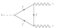
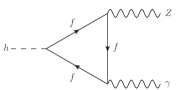
The 2012 discovery of the Higgs boson ($h$) marked a milestone in particle physics [1, 2]. Various properties of $h$ predicted by the standard model (SM) have been confirmed, but there are still many more to be tested. Notable ones are the $h\to\gamma\gamma$ and $h\to Z\gamma$ [3, 4, 5, 6, 7]. They are generated at loop level in both the SM and new physics (NP) [8, 9], making them ideal places to test NP theories hiding at loop level. In particular, $h\to\gamma\gamma$ has been measured to good precision, playing a significant role in probing the Higgs boson [10, 11]. However, $h\to Z\gamma$ has yet to be confirmed experimentally. The triangle Feynman diagrams induced by fermions are given in FIG. 1. As they involve the Yukawa couplings of Higgs boson to fermions, the potential influence of NP beyond the SM in these processes is a compelling aspect of ongoing research [12, 13, 14, 15, 16, 17, 18, 19].

To gauge how well the SM prediction fits data, it is convenient to define the signal strength, denoted as $\mu=(\sigma\cdot{\cal B})_{\mathrm{obs}}/(\sigma\cdot{\cal B})_{\mathrm{SM}}$. This value represents the observed product of the Higgs boson production cross section ($\sigma$) and its branching ratio (${\cal B}$) normalized by the SM values. When $\mu$ deviates from 1, it is a signal of NP beyond the SM. Recently, both ATLAS and CMS [20, 21] have obtained evidence of $h\to Z\gamma$ with the average data showing that

where $\mu_{Z}$ denotes the signal strength of $h\to Z\gamma$. The central value indicates an excess approximately twice as large as that predicted by the SM. On the other hand, the SM prediction aligns very closely with the data of the $h\to\gamma\gamma$ signal strength [22, 23]

At present, the excess for $h\to Z\gamma$ is only at 1.7$\sigma$. If the excess is further confirmed, it will be a signal of NP. In general, for a given NP model addressing the $h\to Z\gamma$ excess, it also affects the process $h\to\gamma\gamma$. Since the measured $\mu_{\gamma}$ agrees well with the SM prediction, the model is severely constrained. For a specific NP model, the literature notably shows that it is difficult to simultaneously align both $\mu_{\gamma}$ and $\mu_{Z}$ with the data within $1\sigma$ [18, 16, 15]. In this work, we study the implications from a model building point of view for the possible $h\to Z\gamma$ excess problem, the issue of the SM expected branching ratio for $h\to\gamma\gamma$ and an excess for $h\to Z\gamma$.

Beyond the SM effects can come in many different ways. In the SM effective field theory, the leading CP-even dimension-six operators contributing to $h\to\gamma\gamma$ and $h\to Z\gamma$ are given as [24]

where $H$ is the Higgs doublet with quantum numbers $(1,2,1/2)$ under the SM gauge group $SU(3)_{c}\times SU(2)\times U(1)_{Y}$, and the vacuum expectation value (vev) is given by $\langle H\rangle=(0,v/\sqrt{2})^{T}$ after spontaneous symmetry breaking. $\Lambda$ represents the energy scale of NP, $c_{BB,WB,WW}$ are identified as the Wilson coefficients, $\tau_{a}$ is the Pauli matrix. With the gauge couplings $g^{\prime}$ and $g$, $B^{\mu\nu}=\partial^{\mu}B^{\nu}-\partial^{\nu}B^{\mu}$ and $W^{\mu\nu}_{a}=\partial^{\mu}W_{a}^{\nu}-\partial^{\nu}W_{a}^{\mu}+g\epsilon_{abc}W_{b}^{\mu}W_{c}^{\nu}$ are gauge field tensors for $U(1)_{Y}$ and $SU(2)$ , respectively. Here we take these operators as examples to show how the excess for $\mu_{Z}^{\text{exp}}$ can be explained. For a full basis that includes CP-violating operators, one may refer to Refs. [8, 25].

After spontaneous symmetry breaking, $B_{\mu}=A_{\mu}\cos\theta_{W}+Z_{\mu}\sin\theta_{W}$ and $W_{\mu}^{3}=Z_{\mu}\cos\theta_{W}-A_{\mu}\sin\theta_{W}$, we could match the above NP operators to the effective Lagrangian responsible to $h\to\gamma\gamma$ and $h\to Z\gamma$ to obtain

with

In the above $\theta_{W}$ is the Weinberg angle, $\alpha_{em}$ is the fine structure constant, $F^{\mu\nu}=\partial^{\mu}A^{\nu}-\partial^{\nu}A^{\mu}$ and $Z^{\mu\nu}=\partial^{\mu}Z^{\nu}-\partial^{\nu}Z^{\mu}$.

Including QCD corrections [26, 27, 28, 29, 30, 31], the amplitudes from the SM are effectively encapsulated by $c_{\gamma}^{\text{SM}}=-6.56$ and $c_{Z}^{\text{SM}}=-11.67$ with $m_{h}=125.1$ GeV. It is noteworthy that $\delta c_{\gamma}$ and $\delta c_{Z}$ are influenced by $c_{BB,WB,WW}$ in distinct ways. The experimental values for $c_{\gamma}$ and $c_{Z}$ can be accomplished by fine-tuning the NP coefficients to induce a minimal $\delta c_{\gamma}$ but sizable $\delta c_{Z}$. We stress that ${\cal L}_{\text{eff}}^{h\gamma\gamma}$ and ${\cal L}_{\text{eff}}^{hZ\gamma}$ are $U(1)_{em}$ gauge invariant, and it suffices to exclusively consider these two for our purpose.

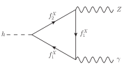
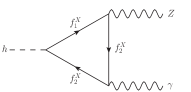
From the above analysis, it is clear that by tuning $c_{BB}$, $c_{WW}$ and $c_{WB}$ it is possible to simultaneously fit the measured data for $h\to\gamma\gamma$ and the excess in $h\to Z\gamma$. Comprehensive studies on the numerical fit within the framework of the SM effective field theory have been carried out [25, 32, 33, 34]. However, it is still a challenging task to solve the excess problem for $h\to Z\gamma$ with a renormalizable model. In a renormalizable model, $\delta c_{\gamma}$ and $\delta c_{Z}$ are generated at one loop level as shown in Figure 1. In this work, we will focus on constructing a renormalizable model to address the problem. We find that a minimally extended model with two fermion singlets and a doublet, as shown in Table 1, can explain the $h\to Z\gamma$ problem. We only consider color-singlet fermions because, otherwise, they would lead to dramatic changes in the $gg\to h$ process and its $p_{T}$ spectrum, in contrast to the data [36, 35, 37]. Two solutions were found. One suggests that the SM amplitude $c_{Z}^{\text{SM}}$ is enhanced by $\delta c_{Z}$ for $h\to Z\gamma$ to the observed value, however, for $h\to\gamma\gamma$, the decay amplitude $c_{\gamma}^{\text{SM}}+\delta c_{\gamma}$ is modified to $-c_{\gamma}^{\text{SM}}$ to give the observed branching ratio. This solution seems to be a contrived solution, although it cannot be ruled out simply using branching ratio measurements. We, however, find another solution which naturally enhances the $h\to Z\gamma$ to the measured value, while keeping the amplitude of $h\to\gamma\gamma$ close to its SM prediction. The model suggests the existence of three new fermions that primarily decay into another fermion and a SM gauge boson. Additionally, it proposes a stable fermion with an electric charge close to $-8$ and masses around 2 TeV.

The new fermions can couple to the Higgs doublet $H$ and can also have bare masses. The Yukawa interaction and bare mass terms are given by

where $\tilde{H}=i\tau_{2}H^{*}$. Without loss of generality, we choose the chiral basis in this work such that terms of the form $m\overline{f}\gamma_{5}f^{\prime}$ vanish as detailed in Appendix A. For a general case, it is also possible to have CP-violating terms of the form $\overline{f}\gamma_{5}f^{\prime}H$. In Appendix A, we outline how the analysis can be carried out. In the following, for clarity and simplicity, we use the above Yukawa coupling to demonstrate how the SM expected branching ratio for $h\to\gamma\gamma$ and an excess for $h\to Z\gamma$ can be realized.

The non-zero vev $v$ of Higgs can contribute to fermion masses leading to the new fermion mass matrices in the basis $(f^{X}_{D},f_{S}^{X})^{T}$ with $X=Y$ or $Y+1$ as the following

The eigenstates $f^{X}=(f_{1}^{X},f_{2}^{X})^{T}$ of $\hat{M}^{X}$ read

where the eigenvalues and mixing angles are

In this basis, the mass and charge-conserved Lagrangian for $f^{X}$ are given as

where $(\eta_{Y},\eta_{Y+1})=(1,-1)$ and $\sigma_{x,y,z}$ are the Pauli matrices operating in the $SU(2)_{L+R}$ rotational space of $f^{X}$. For example, $\overline{f}^{X}\sigma_{x}f^{X}=\overline{f}^{X}_{1}f^{X}_{2}+\overline{f}^{X}_{2}f^{X}_{1}$. On the other hand, the $W$-boson can induce a charge current given by

As we will see shortly, to explain the data we need a large $Y$, which prevents them from coupling with the SM fermions. Hence, the Lagrangian remains invariant under the $U(1)$ rotation of $f_{1,2}^{Y,Y+1}\to e^{i\theta}f_{1,2}^{Y,Y+1}$, and at least one of the new fermions must be stable.

We are ready to calculate the loop-induced $h\to\gamma\gamma$ and $h\to Z\gamma$ in the minimally extended model described previously. The one loop diagrams inducing these decays are shown in Figures 1 and 2. There are two classes of diagrams, one shown in Figure 1 in which the fermions in the loop do not change identities, which we refer to as flavor-conserving ones, and the other as shown in Figure 2 in which the fermions in the loop change identities which we refer to as flavor-changing diagrams. $h\to\gamma\gamma$ receives contributions from the flavor-conserving class, and $h\to Z\gamma$ receives contributions from the both classes. These features make it possible to have NP contributions of the new fermions to $h\to\gamma\gamma$ and $h\to Z\gamma$ differently to addressing the problem we are dealing with.

Depending on the original parameters $m_{D}$, $m_{S}^{X}$ and $c_{f}^{X}$, there are three classes of possible mass eigenstates: 1. both $m_{1,2}^{X}$ are positive; 2. one of the $m^{X}_{1,2}$ is positive and the other is negative; and 3. both $m^{X}_{1,2}$ are negative. In the last case, one can perform a chiral rotation $e^{i\gamma_{5}\pi/2}$ on the fields $f^{X}_{1,2}$ to make all masses positive and transform ${\cal L}_{h}\to-{\cal L}_{h}$, while leaving the other interaction terms unchanged. This would not change the final outcome comparing to the first case, as our final result depends on the value of $(c_{f}^{X})^{2}$. Therefore, we only need to consider the first two possibilities. These two cases can have different features for $h\to\gamma\gamma$ and $h\to Z\gamma$. We proceed to discuss them in the following.

We now provide numerical results for the case with negative $m_{2}^{Y+1}$. For simplicity, we adopt $m_{D}=m_{S}^{Y}=-m_{S}^{Y+1}\,,$ and the masses are given by

Without loss of generality, we take $m_{1}^{Y}>m_{2}^{Y}$. Hence, we have the hierarchy of $m_{1}^{Y}>|m_{1,2}^{Y+1}|>m_{2}^{Y}$, making $f_{2}^{Y}$ being the stable particle due to the energy conservation. For a meaningful perturbative calculation, we consider only the regions where $(c_{f}^{X}/\sqrt{2})^{2}<4\pi$ and fix $Y=-9$. We also confine the model to have the lightest new charged fermion mass be larger than $1600$ GeV to satisfy the experimental lower bound for $|Q_{f}|$ up to 7 [41].

To find the regions of parameter which fit data well, we define

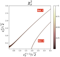
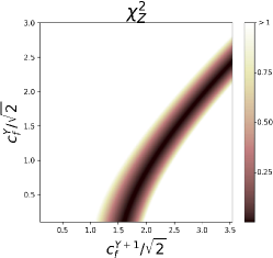
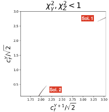
where $\sigma^{\text{exp}}_{\gamma,Z}$ stand for the experimental uncertainties of $\mu_{\gamma,Z}$. In Figure 3(a), (b) and (c), we plot the allowed parameter spaces by setting $\chi_{\gamma}^{2}<1$, $\chi^{2}_{Z}<1$ and $\chi_{\gamma}^{2},\chi_{Z}^{2}<1$, respectively. From Figure 3(a) and (c), it is observed that there are two sets of solutions. We name the upper line Solution 1, characterized by $|\delta c_{\gamma}|\ll|c_{\gamma}^{\text{SM}}|$, while the lower line is named Solution 2, characterized by $\delta c_{\gamma}\approx-2c_{\gamma}^{\text{SM}}$, representing the solution mentioned at the end of the last section. For $\chi^{2}_{Z}$ depicted in Figure 3(b), there is only one set of solutions with $|\delta c_{Z}|<|c_{Z}^{\text{SM}}|$ in contrast. It is worth noting that, if we consider $m_{2}^{Y+1}>0$, there would be no solution here. In the limit of $m_{D}\gg c_{f}^{X}v$, the lines in Figure 3 exhibit a slope of $(Y+1)^{2}/Y^{2}$, necessary to achieve a cancellation between the $f^{Y}$ and $f^{Y+1}$ doublets in Eq. (19).

We also show in Figure 3 (c), the two sets of solutions with the smallest couplings. They are

The corresponding predictions for other parameters are given by

We therefore have found two classes of solutions modify $\mu_{\gamma}$ slightly, but enhance $\mu_{Z}$ to the current average value. Solution 2 seems to be a contrived solution although cannot be ruled out simply using branching ratio measurements. If the current data are confirmed, we would think Solution 1 to be a better solution. It is interesting to point out that due to the large hypercharges introduced, we would encounter the Landau pole in the $U(1)_{Y}$ gauge coupling around 10 TeV in both solutions. If the excess is confirmed, our model will imply additional NP around 10 TeV, which may be detected by future experiments with higher precision and energy. It will be interesting to study which kinds of additional NP we need to remedy the situation.

Due to the smallness of the radiative corrections, we expect the large cancellation in Solution 1 to also occur after including the higher-order corrections. For instance, we consider the next-to-leading order (NLO) QED correction. In the $m_{1,2}^{Y,Y+1}\gg m_{h}$ limit, it shifts the amplitudes by

The formalism can be cross-checked by replacing $Q_{f}^{2}\alpha_{em}$ with $C_{F}\alpha_{s}$ and comparing to the NLO QCD corrections [26, 27], as both have the same topological diagrams at NLO. Since the amplitudes are shifted homogeneously, we conclude that the large cancellations also occur at NLO.

Before ending the discussion, we would like to comment on some other phenomenological aspects at colliders. The new fermions in the model can be produced which has been discussed for smaller $|Y|$ and masses in Ref. [14]. Since in our model the hypercharge $|Y|$ is large, the lightest new fermion is constrained to have a mass larger than $1600$ GeV [41]. The production at the current LHC may be scarce or absent. However, with higher energies and higher luminosity, the new fermions in our model may be produced. The signature of the lightest fermion will leave a charge track in the detector to be measured. While to the heavier ones, if produced they can decay into other final states. For Solution 1, except for $f_{2}^{Y}$ the others will decay into $f_{2}^{Y}$ plus either a $W$-boson or $Z$-boson. But these decays will have large widths of the order of hundreds GeV, making detection difficult since there will not be a sharp resonance peak to look for. On the other hand, for Solution 2, the fermion mass differences are not high enough to form an on-shell gauge boson. They decay into an off-shell $W$-boson, which then decays into a charged lepton and a neutrino, with the decay widths being on the order of a few tens of MeV. Similarly, the decay widths to light quark jet pairs are twice as large. Such measurements may provide information to distinguish between the two solutions.

The signal strengths for $h\to ZZ^{*}$ ($\mu_{ZZ}$) and $h\to WW^{*}$ ($\mu_{WW}$), normalized to the SM predictions, are measured to be $1.02\pm 0.08$ and $1.00\pm 0.08$ [42], respectively. In the SM, these processes are predominantly driven by tree-level couplings, while our model influences them at the NLO through triangular fermionic loops. For both Solutions 1 and 2, the effects on $\mu_{WW}$ are highly suppressed by $(v/m_{1,2}^{X})$ and $\alpha_{em}$, with corrections below the one percent level. The correction to $\mu_{ZZ}$ suffers the same suppression but is amplified by the large $Y$. However, in Solution 1, the destructive mechanism responsible for the small $\delta c_{\gamma}$ occurs also in $\mu_{ZZ}$, leading to correction below one percent. In contrast, Solution 2 delivers the largest correction, with $\mu_{ZZ}-1=3\%$, but is still much smaller than the current experimental precision of $8\%$. To probe the footprints of NP and CP violation, it would be useful to study the $p_{T}$ spectrum of cascade decays of gauge bosons. A comprehensive analysis should be carried out once future experiments achieve the required precision.

We have studied a possible explanation for the $h\to Z\gamma$ excess observed in recent measurements by ATLAS and CMS through the construction of a renormalizable model. If this excess is confirmed, it would be a signal of NP beyond the SM. For NP contribution, while modifying $h\to Z\gamma$, in general it also affects $h\to\gamma\gamma$. Since the measured $\mu_{\gamma}$ agrees well with the SM prediction, there are tight constraints on theoretical models trying to simultaneously explain data on $h\to\gamma\gamma$ and $h\to Z\gamma$. We find that a minimally fermion singlets and doublet extended NP model can explain simultaneously the current data on these decays. We have identified two solutions. One is the SM amplitude $c_{Z}^{\text{SM}}$ is enhanced by $\delta c_{Z}$ for $h\to Z\gamma$ to the observed value, but the $h\to\gamma\gamma$ amplitude $c_{\gamma}^{\text{SM}}+\delta c_{\gamma}$ is modified to $-c_{\gamma}^{\text{SM}}$ to give the observed branching ratio. This seems to be a contrived solution, although it cannot be ruled out simply using branching ratio measurements. We, however, have found another solution which naturally enhances the $h\to Z\gamma$ to the measured value, but keeps the $h\to\gamma\gamma$ close to its SM prediction. With high energy colliders which can produce these new heavy fermions, by studying the decay patterns of the heavy fermions, it is possible to distinguish the two solutions we found. We eagerly await future data to provide more information.

References

- [1] G. Aad et al. [ATLAS collaboration], Phys. Lett. B 716, 1-29 (2012) [arXiv:1207.7214 [hep-ex]].
- [2] S. Chatrchyan et al. [CMS collaboration], Phys. Lett. B 716, 30-61 (2012) [arXiv:1207.7235 [hep-ex]].
- [3] J. R. Ellis, M. K. Gaillard and D. V. Nanopoulos, Nucl. Phys. B 106, 292 (1976).
- [4] R. N. Cahn, M. S. Chanowitz and N. Fleishon, Phys. Lett. B 82, 113-116 (1979).
- [5] M. A. Shifman, A. I. Vainshtein, M. B. Voloshin and V. I. Zakharov, Sov. J. Nucl. Phys. 30, 711-716 (1979) ITEP-42-1979.
- [6] M. B. Gavela, G. Girardi, C. Malleville and P. Sorba, Nucl. Phys. B 193, 257-268 (1981).
- [7] L. Bergstrom and G. Hulth, Nucl. Phys. B 259, 137-155 (1985) [erratum: Nucl. Phys. B 276, 744-744 (1986)].
- [8] J. Elias-Miró, J. R. Espinosa, E. Masso and A. Pomarol, JHEP 08, 033 (2013) [arXiv:1302.5661 [hep-ph]].
- [9] A. Dedes, K. Suxho and L. Trifyllis, JHEP 06, 115 (2019) [arXiv:1903.12046 [hep-ph]].
- [10] [CMS collaboration], CMS-PAS-HIG-13-005.
- [11] G. Aad et al. [ATLAS collaboration], Phys. Lett. B 726, 88-119 (2013) [erratum: Phys. Lett. B 734, 406-406 (2014)] [arXiv:1307.1427 [hep-ex]].
- [12] N. Bizot and M. Frigerio, JHEP 01, 036 (2016) [arXiv:1508.01645 [hep-ph]].
- [13] Q. H. Cao, L. X. Xu, B. Yan and S. H. Zhu, Phys. Lett. B 789, 233-237 (2019) [arXiv:1810.07661 [hep-ph]].
- [14] D. Barducci, L. Di Luzio, M. Nardecchia and C. Toni, JHEP 12, 154 (2023) [arXiv:2311.10130 [hep-ph]].
- [15] G. Lichtenstein, M. A. Schmidt, G. Valencia and R. R. Volkas, [arXiv:2312.09409 [hep-ph]].
- [16] T. T. Hong, V. K. Le, L. T. T. Phuong, N. C. Hoi, N. T. K. Ngan and N. H. T. Nha, PTEP 2024, no.3, 033B04 (2024) [arXiv:2312.11045 [hep-ph]].
- [17] R. Boto, D. Das, J. C. Romao, I. Saha and J. P. Silva, Phys. Rev. D 109, no.9, 095002 (2024) [arXiv:2312.13050 [hep-ph]].
- [18] N. Das, T. Jha and D. Nanda, [arXiv:2402.01317 [hep-ph]].
- [19] K. Cheung and C. J. Ouseph, [arXiv:2402.05678 [hep-ph]].
- [20] A. Tumasyan et al. [CMS collaboration], JHEP 05, 233 (2023) [arXiv:2204.12945 [hep-ex]].
- [21] G. Aad et al. [ATLAS and CMS collaboration], Phys. Rev. Lett. 132, no.2, 021803 (2024) [arXiv:2309.03501 [hep-ex]].
- [22] [ATLAS collaboration], ATLAS-CONF-2019-029.
- [23] A. M. Sirunyan et al. [CMS collaboration], JHEP 07, 027 (2021) [arXiv:2103.06956 [hep-ex]].
- [24] A. Y. Korchin and V. A. Kovalchuk, Phys. Rev. D 88, no.3, 036009 (2013) [arXiv:1303.0365 [hep-ph]].
- [25] A. Pomarol and F. Riva, JHEP 01, 151 (2014) [arXiv:1308.2803 [hep-ph]].
- [26] H. Q. Zheng and D. D. Wu, Phys. Rev. D 42, 3760-3763 (1990).
- [27] M. Spira, A. Djouadi and P. M. Zerwas, Phys. Lett. B 276, 350-353 (1992).
- [28] M. Spira, A. Djouadi, D. Graudenz and P. M. Zerwas, Nucl. Phys. B 453, 17-82 (1995) [arXiv:hep-ph/9504378 [hep-ph]].
- [29] A. Djouadi, Phys. Rept. 457, 1-216 (2008) [arXiv:hep-ph/0503172 [hep-ph]].
- [30] R. Bonciani, V. Del Duca, H. Frellesvig, J. M. Henn, F. Moriello and V. A. Smirnov, JHEP 08, 108 (2015) [arXiv:1505.00567 [hep-ph]].
- [31] T. Gehrmann, S. Guns and D. Kara, JHEP 09, 038 (2015) [arXiv:1505.00561 [hep-ph]].
- [32] S. Dawson and P. P. Giardino, Phys. Rev. D 97, no.9, 093003 (2018) [arXiv:1801.01136 [hep-ph]].
- [33] J. Ellis, C. W. Murphy, V. Sanz and T. You, JHEP 06, 146 (2018) [arXiv:1803.03252 [hep-ph]].
- [34] J. de Blas, Y. Du, C. Grojean, J. Gu, V. Miralles, M. E. Peskin, J. Tian, M. Vos and E. Vryonidou, [arXiv:2206.08326 [hep-ph]].
- [35] M. Battaglia, M. Grazzini, M. Spira and M. Wiesemann, JHEP 11, 173 (2021) [arXiv:2109.02987 [hep-ph]].
- [36] G. Aad et al. [ATLAS collaboration], Nature 607, no.7917, 52-59 (2022) [erratum: Nature 612, no.7941, E24 (2022)] [arXiv:2207.00092 [hep-ex]].
- [37] A. Hayrapetyan et al. [CMS], Phys. Lett. B 857, 138964 (2024) [arXiv:2403.20201 [hep-ex]].
- [38] Q. Bonnefoy, L. Di Luzio, C. Grojean, A. Paul and A. N. Rossia, JHEP 07, 189 (2021) [arXiv:2011.10025 [hep-ph]].
- [39] G. Passarino and M. J. G. Veltman, Nucl. Phys. B 160, 151-207 (1979).
- [40] H. H. Patel, Comput. Phys. Commun. 197, 276-290 (2015) [arXiv:1503.01469 [hep-ph]].
- [41] G. Aad et al. [ATLAS collaboration], Phys. Lett. B 847, 138316 (2023) [arXiv:2303.13613 [hep-ex]].
- [42] R. L. Workman et al. [Particle Data Group], PTEP 2022, 083C01 (2022).