The size–mass and other structural parameter () relations for local bulges/spheroids from multicomponent decompositions
Abstract
We analyse the bulge/spheroid size–(stellar mass), –, relation and spheroid structural parameters for 202 local (predominantly ) galaxies spanning – and from multicomponent decomposition. The correlations between the spheroid Sérsic index (), central surface brightness (), effective half-light radius (), absolute magnitude () and stellar mass () are explored. We also investigate the consequences of using different scale radii, , encapsulating a different fraction (, from 0 to 1) of the total spheroid luminosity. The correlation strengths for projected mass densities, and , vary significantly with the choice of . Spheroid size () and mass () are strongly correlated for all light fractions . We find: with a small scatter of in the direction. This result is discussed relative to the curved size–mass relation for early-type galaxies due to their discs yielding larger galaxy radii at lower masses. Moreover, the slope of our spheroid size–mass relation is a factor of , steeper than reported bulge size–mass relations, and with bulge sizes at M⊙ which are 2 to 3 times smaller. Our spheroid size–mass relation present no significant flattening in slope in the low-mass end (–). Instead of treating galaxies as single entities, future theoretical and evolutionary models should also attempt to recreate the strong scaling relations of specific galactic components. Additional scaling relations, such as –, –, and –, are also presented. Finally, we show that the local spheroids align well with the size-mass distribution of quiescent galaxies at –. In essence, local spheroids and high- quiescent galaxies appear structurally similar, likely dictated by the virial theorem.
keywords:
galaxies: bulges – galaxies: elliptical and lenticular, cD – galaxies: structure – galaxies: evolution1 Introduction
Some of the complexity in galaxy morphology arises from the different developmental processes of the ellipsoidal/spherical bulge and flat disc. Their diametrically different nature leads to the support for a two phase formation scenario (e.g., Graham, 2013; Driver et al., 2013), where the bulges were formed via a rapid, hot-mode process (early collapse) at high-redshifts (e.g., Naab et al., 2009; Hopkins et al., 2009; Bezanson et al., 2009; Trujillo et al., 2011) and the discs are subsequently built through mergers and accretion (Larson, 1976; Tinsley & Larson, 1978; Graham et al., 2015, and reference therein). In this picture, massive bulges formed first () and the disc later, a.k.a., an inside-out evolution. Less massive galaxies may have experienced a delayed, more gradual evolution in a down-sizing scenario (e.g. Graham et al., 2017). The third phase of evolution will be the major merging of these galaxies to produce elliptical (E) galaxies or S0 galaxies if the net angular momentum is not sufficiently cancelled.
While the bulges of some of today’s massive galaxies appear to be the descendants of the high- compact massive galaxies (such as NGC 3311, see Barbosa et al., 2021), some lower mass bulges may also have existed as smaller "red gems" in the distant Universe. Indeed, the stellar population in the inner part of galaxies seems to be significantly older than the outer region (Proctor & Sansom, 2002; Moorthy & Holtzman, 2006; Thomas & Davies, 2006; Jablonka et al., 2007; MacArthur et al., 2008; Saracco et al., 2009), with the work by MacArthur et al. (2009) revealing that the bulk of the stars in spiral galaxy bulges are old.
Early-type galaxies (ETGs) are known to follow a curved size-mass relation, stretching from the ellipitcal (E) galaxies at the high-mass end (Caon et al., 1993; D’Onofrio et al., 1994; Shen et al., 2003; Cappellari et al., 2011a; Baldry et al., 2012; Lange et al., 2015, 2016; Morishita et al., 2017; Nedkova et al., 2021; Noordeh et al., 2021) to the dwarf ETGs (dETGs) at the low-mass end (Binggeli & Jerjen, 1998; Graham et al., 2006; Forbes et al., 2008; Graham, 2013). Due to the prevalence of discs in ETGs (Scott et al., 2015, and reference therein), this curved relation is a product of the disc size and mass, which dominate the ETGs at the low-mas end. In the 70s, when the galaxies’ size was measured using isophotal radius (e.g., Heidmann, 1969; Holmberg, 1969; Oemler, 1976; Strom & Strom, 1978), the galaxies exhibited a linear size-mass relation in log-log space (i.e., the size–mass relation follows a simple power law)111Evidence of a linear isophotal size–mass relation are also seen in later works (e.g., Forbes et al., 2008; van den Bergh, 2008; Nair et al., 2011).. However, these works primarily focus on the size-mass relation for galaxies as a whole instead of their substructures. Additional insight can be drawn if a similar study is conducted on the bulge/spheroids. A bulge/bar/disc decomposition is required to explore the size–mass relation of ETG bulges, as opposed to the size–mass relation of the galaxies themselves. This enables greater insight into the formation physics shaping the components of galaxies. Before high-resolution observations of distant galaxies, such as those promised by MAVIS (optical, under development, McDermid et al. 2020; Rigaut et al. 2020) and VLT’s PIONIER (1.6 , Le Bouquin et al. 2011), and GRAVITY (2.0–2.4 imager, Gillessen et al. 2010; Eisenhauer et al. 2011) are available, local spheroids are a great place to probe the Universe’s past. Important questions can be asked in regard to bulge formation. For instance, with the low merger rate at (De Propris et al., 2005, 2007; De Propris et al., 2010), how are spheroids formed so efficiently 10–12 Gyr ago? Is the continuity in the spheroid size–mass relation, from E galaxies to spheroids embedded in S0, S, and dETGs, a coincidence, or are they the products of the same formation physics but simply differ in scale?
For decades, the standard method to break down galaxy structure was to fit either an (de Vaucouleurs, 1948) or an (Sérsic, 1968) model to describe the spheroid, plus an exponential function to describe the disc (e.g., Andredakis et al., 1995; Seigar & James, 1998; Iodice et al., 1999; Khosroshahi et al., 2000b; D’Onofrio, 2001; Graham, 2001; Möllenhoff & Heidt, 2001; Simard et al., 2002; Allen et al., 2006; Fisher & Drory, 2010; Simard et al., 2011, etc.). However, due to the complex substructures in galaxies, a simple Bulge+Disc decomposition is inappropriate for some. Consequently, past size–mass relations for bulges are questionable due to the influence of, for example, the bar, which can inflate both the size and the mass of the presumed ‘bulge’ component. This can muddy the waters when attempting to identify classical bulges versus ‘pseudo-bulges’. Given the need for more detailed breakdowns of galaxy structures, many (e.g., Martin, 1995; Prieto et al., 1997; Aguerri et al., 1998; Graham et al., 2003b; Laurikainen et al., 2005; Gadotti, 2009; Laurikainen et al., 2010; Vika et al., 2012; Läsker et al., 2014; Savorgnan & Graham, 2016a; Davis et al., 2019; Sahu et al., 2019) developed sophisticated, manual (i.e., not blind automated) multicomponent decompositions in an attempt to capture these substructures. The benefit of such, interestingly, is that now the spheroids can be better qualified because the biasing substructures have been accounted for.
While spheroids can grow, the entropy of such pressure-supported systems makes them hard to erase. As such, they are expected to have longevity which bars and spiral arms will not. Here, we focus on the spheroids, leaving the bar or disc scaling relation for future investigation. We take advantage of multicomponent decompositions to examine the bulge/spheroid size-mass (–) relation and some of their structural parameters: central surface brightness () and Sérsic index ().
In Section 2, we briefly describe our data sources (Section 2.1), the surface brightness profile extraction (Section 2.2), and the models used to measure the spheroids (Section 2.3). In Section 3, we first discuss the spheroid structural parameters and their correlations with each others (Section 3.1 and 3.2). We subsequently explore the changes among these parameters when using scale radii enclosing different fractions of the spheroid light (Section 3.3). Subsequently, we converted the spheroid absolute magnitude into stellar mass (Section 3.4) and studied how the spheroid mass related scaling relations varies when using different scale radii (Section 3.4.1, 3.4.2, and 3.4.3). The spheroid size-mass relation (Section 3.5.1) and other scaling relations (Section 3.5.2) are also presented. Section 4 compares the spheroid size-mass relation to relevant works in the literature and discusses what it informs us on the formation history of the spheroids.
2 Data and Analysis
2.1 Galaxy sample
We utilise the following works for our analyses: (1) Savorgnan & Graham (2016a, hereafter SG16), (2) Davis et al. (2019, hereafter D+19), (3) Sahu et al. (2019, hereafter S+19), and (4) Hon et al. (2022, hereafter H+22). These studies have performed physically-motivated222Rather than blindly fitting 2, 3, or 4 Sérsic components, we inspect each image and fit for specific physical components seen in the data., multicomponent decompositions of local galaxies of various morphology. The decomposition in D+19, S+19, and H+22 are performed using Profiler (Ciambur, 2016), while SG16 used their own programme "profilterol".
Among the data from the four works, there are some repeating galaxies. There is one galaxy in D+19 (NGC 3368) and four galaxies in S+19 (NGC 3665, NGC 4429, NGC 4526, and NGC4649) overlapping with H+22. We adopt the newer decomposition from H+22 and remove the repeating data points from the previous works. In total, there are 241 unique galaxies in these data sets. See the respective papers for the structural parameters of individual galaxies. The followings are brief descriptions of each.
2.1.1 Savorgnan & Graham (2016)
SG16 analyzed 66 galaxies with dynamically measured supermassive black hole (SMBH) mass, , from Greenhill et al. (2003); Graham & Scott (2013); Rusli et al. (2013). It contains 47 ETGs and 19 "early-type" spiral galaxies. The analysis was performed on Spitzer/IRAC (InfraRed Array Camera) images (Fazio et al., 2004; Werner et al., 2004) (see SG16, their Section 2.1). In their subsequent paper, Savorgnan et al. (2016) convert the luminosity into stellar mass using a constant mass-to-light (, or ) ratio of (Meidt et al., 2014)333Meidt et al. (2014) assumes a Chabrier (2003) initial mass function (IMF), a Bruzual & Charlot (2003) stellar synthesised stellar population model (SSP), and an exponentially declining stellar formation history (SFH)..
2.1.2 Davis et al. (2019)
D+19 performed multicomponent decompositions for 43444Three of which are bulgeless galaxies. late-type galaxies (LTGs). The sample was selected based on a compilation from Davis et al. (2017): a set of spiral galaxies with their SMBH mass measured via proper stellar motion, stellar dynamics, gas dynamics, and stimulated astrophysical masers (see their Table 1). The spiral galaxy data set consists of the following morphological type: 10 SA, 12 SAB, and 22 SB galaxies (defined by RC3 de Vaucouleurs et al., 1991)555Four of which were discarded by D+19 in the decomposition process.. D+19 analysed the galaxy structures primarily using images. D+19 analyzed the Spitzer Survey of Stellar Structure in Galaxies (, Sheth et al., 2010) and the Spitzer Heritage Archive (SHA)666http://sha.ipac.caltech.edu. Alternative data from the -band in Hubble Space Telescope (HST)777https://mast.stsci.edu/ images and -band images from the Two Micron All Sky Survey (2MASS) Large Galaxy Atlas (LGA, Jarrett et al., 2003) were used in the absence of Spitzer images or when greater special resolution was required (see Section 2.2 in D+19). In LTGs, because the dust in the disc glows in the infrared, D+19 used a smaller stellar mass-to-light ratio , in accordance with data from Querejeta et al. (2015), to compensate for the potential overestimation of stellar mass due to non-stellar luminosity in LTGs (see Section 2.8 in D+19)888D+19 used the median from Fig. 10 of Querejeta et al. (2015) and the color-independent from Meidt et al. (2014) to estimate the median value of . See Section 2.8 in D+19 for details.. For the sake of consistency, we only use their 26 galaxies with Spitzer images.
2.1.3 Sahu et al. (2019)
Building upon the 47 ETGs from SG16, S+19 added 41 more ETGs, including seven remodelled ETGs (A3565 BCG, NGC 524, NGC 2787, NGC 1374, NGC 4026, NGC 5845, and NGC 7052). For these seven remodelled galaxies, we use the parameters provided by S+19. Among the newly added 41 galaxies, based on their decomposition, are 15 E, 3 ES, and 23 S0 galaxies, respectively. S+19 data sources are from: -band images in Spitzer/IRAC (Sheth et al., 2010), r-band images in Sloan Digital Sky Survey (SDSS, York et al., 2000), -band images from 2MASS/LGA (Jarrett et al., 2003), and -band in SHA. As was done with the D+19 data, we only use the Spitzer galaxies from S+19, which amounts to 33 galaxies.
Similar to what was done in SG16, the spheroid luminosity from Spitzer/IRAC and SHA images are converted into stellar mass with a constant mass-to-light ratio (Meidt et al., 2014, see their Section 3.3 for details).
2.1.4 Hon et al. (2022)
H+22 selected a mass- and volume-limited sample of massive () galaxies at from the NASA-Sloan catalogue999http://www.nsatlas.org/ based on SDSS photometry (York et al., 2000; Aihara et al., 2011) in the -band. The H+22 sample contains 103 massive galaxies with (based on the Roediger & Courteau (2015) ratio) but is otherwise nondiscriminatory to galaxy morphology. According to H+22’s decomposition, the galaxies are assigned new morphologies. There are 13 ellipticals (E+ES)101010Here, the elliptical galaxies are composed of two populations: 11 conventional ellipticals (E) and two ellicular (ES) galaxies. ES galaxies (Liller, 1966; Savorgnan & Graham, 2016b; Graham, 2019b) are ellipitcals that contain an intermediate-scale disc. The name ”ellicular” (”elliptical+lenticular”) was introduced in Graham et al. (2016)., 50 lenticular (S0) and 40 spiral (S) galaxies in this sample. H+22 use the galaxies’ - and -band photometry from SDSS to estimate the ratio. In this paper, we will use the ratio provided by the Roediger & Courteau (2015) prescription, which provides agreement with the Spitzer-derived masses from the three other works (Sahu et al., 2019, see their Section 3.4) 111111The ratio utilised by the four works assume a Chabrier (2003) initial mass function and the stellar population model from Bruzual & Charlot (2003) (see Meidt et al., 2014; Roediger & Courteau, 2015).. After removing the non-Spitzer galaxies from the previous three studies and combining them with H+22, we have, in total, 202 galaxies for analysis.
2.2 Surface brightness profile analysis
The surface brightness profiles of the host galaxies were previously extracted via the isophotal fitting programme ISOFIT (Ciambur, 2015). Built on the isophotal fitting function ellipse in IRAF, it fits a series of concentric quasi-ellipses onto the galaxy image. The flux along each quasi-ellipse gives the surface brightness at a given radius. Improving upon ellipse, ISOFIT is able to better handle bars and near-edge-on discs by correctly using high-order Fourier harmonic distortions to ellipses rather than just circles (see Ciambur, 2015, for details).
The decomposition is informed by the various radial profiles (surface brightness , ellipticity , Position Angle , harmonic coefficients , ) of the galaxy isophotes, describing features in the 2D images. Relevant studies from the literature were also considered when choosing the appropriate components for each galaxy. In addition to the more apparent structures, such as a bulge, extended disc, and bar, less prominent but important substructures, such as a nuclear disc (Ferrarese et al., 1994; van den Bosch, 1998; Scorza & van den Bosch, 1998; Balcells et al., 2007), secondary bar (Buta & Crocker, 1993; Shaw et al., 1993; Wozniak et al., 1995; Jungwiert et al., 1997; Erwin et al., 2003), anase (Martinez-Valpuesta et al., 2007) and rings (Buta & Combes, 1996), were also included in the decomposition (see Section 3 in Hon et al., 2022). The different types of disc, namely the Type I regular disc (Patterson, 1940; de Vaucouleurs, 1957), the down-bending Type II disc (van der Kruit & Searle, 1981), the up-bending Type III disc (de Grijs et al., 2001; Pohlen et al., 2002), and the inclined disc model (van der Kruit & Searle, 1981) were also considered. Because such potentially biasing factors and components have been accounted for, the bulges/spheroids obtained from the decomposition process are more accurate than simple 2-component Bulge+Disc decomposition. Rather than relying on a statistical approach, e.g., Akaike information criterion or Bayesian information criterion, additional components were only fit if there was evidence, either pre-existing in the literature or in the SDSS imaging data, for their presence. This included features in the ellipticity (), position angle () or harmonic coefficient (e.g. , ) radial profiles. For detailed descriptions of the decomposition process, see Sec. 3.3 and Fig. 6 in H+22.
The multicomponent galaxy models were convolved using a Moffat representation of the PSF measured in the same frame as each galaxy. For the SDSS -band images from H+22, the median FWHM size of the PSF is , with individual measurements listed in Tables C1–C3 of H+22. None of the 103 galaxies had . As noted in section 2.2 of D+19, when was comparable to or smaller than the ‘seeing’ of the Spitzer Space Telescope (), then HST data was used for those galaxies with directly measured black hole masses, which are not included here due to our effort to ensure the use of consistent ratios between the samples. This was also the case with the Spitzer sample from SG16 and S+19. That is, the black hole sample used here has a priori excluded galaxies with , and simulations have repeatedly shown that the Sérsic model’s can be recovered under such conditions (Gadotti, 2008).
Finally, it is perhaps useful to remark on the nature of the spheroids, whether they are the classical bulges or pseudo-bulges built via secular influence from the disc. SG16 stated that they did not attempt to distinguish between classical and pseudo-bulges. However, with most of their data being barless S0 galaxies and giant elliptical galaxies, pseudo-bulges are not likely to be present in SG16. Because D+19 focuses on LTGs, they reported on claims in the literature for 35 pseudo-bulges in their sample of 43. However, having their galaxies’ bar components and (peanut shell)-shaped structures captured and modelled, bar-induced pseudo-bulge structures were effectively subsumed into the bar model. D+19 note that all their bulges co-define the same - relation. A tight - relation implies the bulges they extracted are the structures that coevolve with the SMBH, namely the classical spheroids instead of the secularly-built pseudo-bulges. S+19 modelled the boxy/X/(peanut shell)-shaped structure, as well as the oval (barlens) structure, separate from the (classical) bulges. They used either a Ferrers (Ferrers, 1877; Sellwood & Wilkinson, 1993) or Sérsic function (Sérsic, 1968) for these "pseudo-bulge" structures (see in their plots, NGC 4792, NGC 2787, and NGC 4371); that is, the disc-induced, secularly-built pseudo-bulges are captured in either the bar/barlens component. The same treatment can be seen in H+22. Therefore, the spheroids described in this work are thought to be classical bulges and not inner discs, which are modelled as such, nor features thrown up by unstable bars.
2.3 Spheroid model
The spheroids are modelled by either one of two functions: the Sérsic or the core-Sérsic function (Graham et al., 2003a). The Sérsic function describes the bulges’ intensity profile with three parameters (, , and ), such that
| (1) |
where is the Sérsic index or ‘shape parameter’ that depicts the shape of the profile, is the "effective" half-light radius that encapsulate half the total luminosity, and is the intensity at . It is easy to see that . The quantity is a function of , determined by solving the equation , where and are the complete and incomplete gamma functions, respectively (see Graham & Driver, 2005). For , can be approximated by the following equation: (Capaccioli et al., 1989). The total luminosity () can be calculated by integrating the intensity over the projected surface of the galaxy. We have:
| (2) |
and the surface brightness () at a given radius () is:
| (3) |
The Sérsic function has a particular noteworthy construct. The value of is arbitrarily defined in Sérsic (1968) to be the value where the parameter, , encompasses half of the total luminosity (). When switching to a different scale radius, , encompasses a different fraction of the total light, and this is achieved by changing to a new constant . We can convert to using equation 22 in Graham (2019a):
| (4) |
where is a function of obtained by solving the equation , and is the enclosed fraction of light ranging from 0 and 1.
The scale radius, , is often overlooked in the literature. As one chooses to characterise the spheroid structures with a different instead of , the distribution of and projected mass density will change as well. As a result, the corresponding scaling relations differ drastically from when was used. One might incorrectly assign physical significance to a particular relation without realising that some quantities are arbitrarily defined and unrelated to the underlying physics of galaxy evolution. We shall reveal how the correlation strength changes for different scaling relations as a function of light fraction later in Section 3.3.
Similarly, the corresponding surface brightness at , , will be:
| (5) |
where is the central surface brightness. The average surface brightness, , within is:
| (6) |
where, here, we name the function the ‘shape function’121212 Graham (2019a) refer to this function as (see their equation 20). of a Sérsic profile:
| (7) |
Note that is required to calculate the total luminosity of a Sérsic profile with .
The surface brightness, , can be converted into a physical quantity, the projected mass density, :
| (8) |
where is the surface brightness at ; is the distance modulus; is the absolute magnitude of the Sun at wavelength ; is the physical size scale in ; and is the mass-to-light ratio at wavelength (Sahu et al., 2022, see their equation A5 for details).
Some massive galaxies/spheroids have surface brightness profiles which deviate from the Sérsic model because of their core-deficit (King, 1978; Byun et al., 1996; Trujillo et al., 2004). The merging of binary SMBHs ejects the neighbouring stars outwards through gravitational slingshots (Saslaw et al., 1974; Begelman et al., 1980). As a result, the surface brightness profile of the core is shallow out to some "break-radius", , and conforms to a regular Sérsic model in the outer region. For this special class of spheroids, they are modelled with the six parameters () "core-Sérsic" function131313The core-Sérsic function is an empirical model combining a power-law to describe the depleted core with the Sérsic function. (Graham et al., 2003a):
| (9) |
where is the "break-radius", describes the slope of the inner power-law profile, and describes the sharpness of the transition between the inner (power-law) and outer (Sérsic) regimes. The intensity can be expressed as such:
| (10) |
where is the intensity at the break-radius. See Fig. 9 and 10 in Graham et al. (2003a) for the differences in Sérsic and core-Sérsic functions.
In what follows, we present the spheroid scaling relations, as well as their structural parameters as described by these two models. Unless otherwise stated, all parameters (e.g., , ,) shown in this work are calculated using radii, , equivalent to the geometric-mean of the major () and minor () axis: . This implicitly accounts for the ellipticity of the isophotes.
3 Results
This section is structured as follows:
- 1.
- 2.
-
3.
In Section 3.4, we convert the spheroid surface brightness and magnitude into physical quantities: , , and , where and are the stellar surface mass density at and within , and is the spheroid stellar mass. This enables us to fold in the sample from SG16, D+19, and S+19 in to the analysis. In Section 3.4.3, we explore the correlation strength of various quantities: , , , , and with the spheroid stellar mass, , under the assumption of different scale radii.
- 4.
3.1 Absolute Magnitude versus Sérsic index, central surface brightness, and effective radius
Fig. 1 shows the distribution of the total spheroidal absolute magnitude, , versus the Sérsic index, , central surface brightness, , and effective radius, , from the sample in H+22. The core-Sérsic spheroids, highlighted by red circles, are universally bright with in the -band (AB mag). The distribution of spheroid parameters separates E+ES galaxies and spheroids from S0 and S galaxies. In the plot (left-hand panel), most spheroids residing at and are elliptical (E+ES) galaxies. Bulges coming from S0 and S galaxies concentrate in and . In the middle panel of Fig. 1, the – plot presents a rather different distribution. S0 and S spheroids are concentrated between and , while the E+ES galaxies span a different range, at and . These differences likely reflect a major merger origin for the ES/E galaxies, inflating their and luminosity as the disc mass of the progenitors is turned into spheroid mass and resulting in larger Sérsic indices and brighter (extrapolated) values. In practice, the damage caused by coalescing binary SMBHs erodes the central stellar phase space and reduces the observed value. The disc stars from the progenitor galaxies contribute to the long tail of their high- profile. The – relation, shown in the right-hand panel, exhibits a strong log-linear trend, with good agreement across the E+ES, S0 and S bulges. At –, the spheroid population is dominated by E+ES galaxies.

Studies have reported linear scaling relations for ETGs in the – and – planes (Caon et al., 1993; Young & Currie, 1994; Graham et al., 1996; Graham, 2001; Ferrarese et al., 2006; Savorgnan et al., 2013; Janz et al., 2014). For instance, using a single Sérsic function to model ETGs in the -band (Binggeli & Jerjen, 1998; Caon et al., 1993; D’Onofrio et al., 1994; Stiavelli et al., 2001; Graham et al., 2003b). Researchers have investigated the empirical – and – for massive ETGs. In Graham & Scott (2013, see their Fig. 6), both distributions exhibit a clear linear relation (see also their equation 6 and 7), and they use these empirical relations to predict the ETG size–luminosity relation in the -band.
However, for the spheroid structural parameters shown in Fig. 1, the – and – relations are not obviously log-linear. The – relation appears to have a wide range of scatter, and the – distribution has a prominent "bend" at (AB mag), with E+ES galaxies having much brighter central surface brightness compared to the S0 and S bulges. Interestingly, our – distribution is similar to Watkins et al. (2022)’s – relation for their ETGs (see their Fig. 14). While their distribution is also clearly not linear, by excluding galaxies with high Sérsic index (), they provide a linear – relation (see their equations 15–16). Here, we first test the linearity among the three distributions shown in our Fig. 1.
We computed the Pearson correlation coefficient () and the Spearman rank-order correlation coefficient () for each distributions (listed in Fig. 1). The coefficient depicts how well a linear relation describes our data and describes how well the relation approximates a monotonic increasing trend. For our spheroids, both and are similar across all parameters. The – relation presents the highest positive correlation among the three, with and . Note that the coefficient is negative because a more luminous object has a lower absolute magnitude. Following the observation above on the different locations of elliptical and disc galaxies in these scaling diagrams, we subdivided our sample into E+ES and S0+S galaxies to check if there is any deviation between the two groups. The Pearson and Spearman coefficients for ellipticals, and , and disc-galaxies, and , are shown in Fig. 1. Note that, in particular, in the – plane, disc-galaxies exhibit a different pattern than the ellipticals, with and .
3.2 Correlation between and
Beyond comparing structural parameters to the spheroid magnitude, we also study how these parameters relate to each other. Fig. 2 shows the distribution of H+22’s spheroids in the –), – and – planes.
Among the three relations, the distribution in the – plane shows the strongest correlation ( and ). It is remarkably linear, especially for the E+ES galaxies () due to extrapolation of the Sérsic model, with high- profiles giving bright values. In the –) plane, the spheroids exhibit a moderately high correlation (). The shape of the distribution is somewhat reminiscent of that seen in the – diagram in Fig. 1. Given that and are strongly correlated, forming essentially a log-linear relation, it is not surprising that the – distribution resembles the – distribution. The – distribution does not exhibit any obvious scaling relation beyond a broad trend. E+ES galaxies and bulges from S0+S galaxies occupy different regions of the plot with most S0+S bulges within and . A spheroid effective radius, , is not particularly useful in predicting the central surface brightness, .
Two sets of spheroid parameters: – and – have the highest correlation among any pairs and, therefore, can be used as the primary scaling relations to predict spheroid properties reliably. In contrast, – and – relations are moderately correlated with a varying range of scatter. As such, and can be used as a supplementary predictor for the spheroid shape, if is not available.
The – relation is one of the more prominent scaling relations among spheroid parameters. In Khosroshahi et al. (2000a), using both the bulges from two component decompositions of disc galaxies and E galaxies, they found that the – relation, has a high correlation factor of . It suggests the shape of the spheroid’s light profile, measured by the Sérsic index, , dictates the (at least extrapolated) value of its central surface brightness, , or vice versa. However, unlike Khosroshahi et al. (2000a), we found our spheroid – relation to be linear instead of the – relation (, see Fig. 2). In the – plane, our spheroids have a curved relation.

3.3 Alternate scale radii and the associated scale intensities
From this Section onward, we examine the spheroid parameters using alternate scale radii . The local ETGs’ size-mass relation changes slopes at a bending point near the -band magnitude, , when using (e.g., Graham, 2013). Such a feature had been used to argue in favour of distinct formation scenarios between two classes of objects (Kormendy et al., 2009; Tolstoy et al., 2009; Kormendy & Bender, 2012; Somerville & Davé, 2015; Kormendy & Freeman, 2016). However, an extensive review by Graham (2019a) pointed out that the curvature in the galaxy size-mass relation is artificial. As shown in their Section 7 and Fig. 3, the shape of the curved size–mass relation varies drastically when radii that encompass a different, say, 10 or 90 per cent of the light, are chosen, i.e. different scale radii. Moreover, the magnitude at the bend point that supposedly divides ETGs and dETGs galaxies also change accordingly, and therefore the alleged division at carries no physical meaning. To avoid misinterpretation, we shall bare in mind the effect of chosen scale radii on the distribution of the spheroid parameters.
3.3.1 and

In this section, we develop the spheroid – and – relations, with a different definition for the radial scale parameter, , and thus also the intensity scale parameter (). The canonical approach with the Sérsic model is to only use the effective half-light radius . We examine how the various relations change when a different fraction (, from 0 to 1) of the total luminosity, , is used to define the equally-valid alternate scale radii, .
In the left-hand panel of Fig. 3, we show – using a radius encapsulating 50 percent (, red points), 5 percent (, black points) and 95 percent (, blue points) of the light. We illustrate the trends for each relation with green dashed lines. The green points are the median value within an absolute magnitude interval of from to . In the right-hand panel of Fig. 3, the – distributions are presented, where is the surface brightness at . For (purple points), it recreates the same plot as shown in the middle panel of Fig. 1. When , the – relation presents a positive trend, i.e., a brighter spheroid has a more luminous central surface brightness value. For and , both relations change directions and have their absolute magnitude negatively correlating with the surface brightness, (or ) and . In both panels, the spheroids have a continuous relations between to (in -band AB mag). The spheroid population appears to be continuous regardless of the radius used.
3.4 From magnitude to mass
3.4.1 –, – and – relations
In an effort to extract physical meaning from these relations, as well as comparing the data from H+22 with SG16, D+19 and S+19, we converted the spheroids’ absolute magnitude, , into stellar mass, , and central surface brightness, , into central projected mass density, . Using the data from the four sources, we plotted the spheroid stellar mass, , versus Sérsic index, , , and in the left-hand, middle, and right-hand panel in Fig. 4, respectively.
Kelvin et al. (2012, their Fig.22) report how the galaxy half-light radii change with wavelength, which is related to the bulge/disc transition, such that the (small) different colours between the bulge and disc can produce a change in the galaxy size as a function of wavelength (Kennedy et al., 2016). Kelvin et al. (2012) report that the drop in the median galaxy size from the -band (0.6 micron) to the , , and -band (1-2 micron) is 4.5 kpc to 3.5 kpc, before the decline in size stabilises beyond 1 micron. This is a 22% drop, or 0.11 dex, for the galaxy half-light size. Vulcani et al. (2014) performed the same analysis, and for their ‘red galaxies’, the median galaxy size dropped from 5.5 kpc to 4 kpc (0.14 dex) when going from the -band (0.6 micron) to the -band (1.6 micron). However, what is required is the change in the bulge/spheroid size rather than the change in the galaxy (bulge+disc+bar) size. As discussed in Hon et al. (2022), for a uniform stellar population within the spheroidal component, there should be no systematic change in the spheroid’s size with wavelength, modulo the impact of dust. We are, however, at present unable to quantify this change from the -band to 3.6 microns, and as such, have not implemented any rescaling of the spheroid sizes.
The correlation coefficients for the entire sample, and , where "All" now includes all four galaxy samples (SG16, D+19, S+19, and H+22) in both –, –, and – planes are comparable to that in the –, –, and – planes from Fig. 1, respectively. The inclusion of the data from SG16, D+19 and S+19 does not increase the correlation strength. In the – plane, when we divide the sample into ellipticals and disc-galaxies, both subgroups return an extremely low correlation, with and . The weak correlations between the spheroid luminosity (subsequently its stellar mass) and projected central density persists even after being converted into physical quantities, and . Sahu et al. (2022) reported a similar Pearson correlation coefficient, (their table 1), in the – plane. Due to the coevolution between the SMBH and the spheroid, and are strongly correlated. Therefore, the similarity between the – and – relation is somewhat expected.
In Fig. 5, we convert the – and – into the – and – distributions by using different scale radii, encompassing light fractions and . The behaviour is similar to that in Fig. 3. The – distributions maintain a somewhat linear trend with positive slope while the – distributions change slope with different values of .
3.4.2 – relation
Some studies have suggested that the average projected mass density within a small fixed radius, say 1 kpc, , or 5 kpcs, , are great estimators to track the growth of SMBHs (e.g., Barro et al., 2017; Dekel et al., 2019; Ni et al., 2021; Sahu et al., 2022). By proxy, it will also pertain to the growth of spheroids, given the connection between the two. Indeed, the – plane exhibits a log-linear relation ( and , see Sahu et al., 2022). However, it is noteworthy that at this fixed radius, the quantity might be sampling a different percentage of light in different spheroids. For instance, for a bulge with , captures nearly half of the light, while for a spheroid like an E galaxy with , it captures a small fraction. In the interest of studying how the average projected mass density141414 can be calculated by subsituting (see equation 6) into equation 8., , varies as one includes a different percentage of light within the radius , we plot versus in Fig. 6. The – relations present a negative trend for all . This result is consistent with Sahu et al. (2022) who found a negative correlation in the – () relation (see their Fig. 6). As the value of increases, the – relation appears increasingly more linear and has a steeper slope. In addition, it appears that the correlation strength of the distributions varies with . At , the correlation is non-existent () while at , and have a moderate correlation ().
Since is calculated by substituting with in equation 8, the varying trends in the – plane can be explained by looking into the formulation in equation 6. The average surface brightness, , is a linear combination of the surface brightness, , in the first term and the shape function, , in the second term. Because is purely a function of Sérsic index , it inherits the moderately strong linearity in the – plane (see Fig. 4). We demonstrate such a strong trend in Fig. 7, where the spheroid stellar mass () is plotted against . Indeed, the – relations have a rather consistent anti-correlation151515The negative sign is due to the multiplier . Spheroid stellar mass, correlates positively with the shape function . across , with . Hence, the variation in correlation strength in the – plane is because of the inherent non-linearity in the – relation (see Fig. 1). This latter trend dampens the correlation strength of the – distribution and results in an changed trend as changes. It is clear that the choice of the light fraction value significantly affects the shape and slope of the scaling relations.


3.4.3 Correlation strength ( & ) versus fraction
Here, we explore how the correlation strength changes with different light fractions . In Fig. 8, we plot the correlation strength, and , in the upper and lower panel, respectively, as a function of the fraction of spheroid light, , contained within the radius , for various scaling relations: –, –, –, and –, where all involve the stellar mass. The – relations (green line) are consistently strongly coupled regardless of the value of . The – relation (blue line) is positively correlated at , but it becomes negatively correlated at larger , a feature that can be seen in the right-hand panel of Fig. 5. For the – relation at (first point on the red line), it has an extremely low correlation () but as increases, it becomes increasingly anti-correlated. Finally, the – relations (purple line) exhibit a very consistent anti-correlation trend across all with .
Fig. 8 provides an important insight into spheroid scaling relations that, in general, the surface brightness, , and its derived physical quantities ( and ) are comparatively weak estimators for spheroid stellar mass. While the scaling relations become more reliable at higher light fraction , the correlation coefficients are limited to . The variability in correlation strength across makes these scaling relations inherently biased by choice of .
In Section 3.1, we found that the Sérsic index () of a spheroid is a slightly better predictor for a spheroid stellar mass than . Here, we show that the Sérsic shape function, , is also a decent spheroid mass predictor across all (). Similarly, also has a consistently strong log-linear relation with across all but with an even higher correlation strength (). Hence, we advocate using as the primary predictor to spheroid stellar mass () and (or ) as the secondary. Of course, , , and perfectly define the stellar luminosity of the spheroid.


3.5 Fitting the scaling relations
3.5.1 The spheroid size–mass (–) scaling relation


With the above observation that spheroid size () is the most consistent and reliable predictor for spheroid stellar mass () across all , we proceed to investigate the spheroid size-mass relation for our expanded sample. In Fig. 9, we present the equivalent axis effective radius () versus the stellar mass () for the local spheroids from SG16, D+19, S+19, and H+22. In the left-hand panel of Fig. 9, the data is separated by the morphological type of the host galaxies. There is a significant overlap between S0 and S spheroids. The elliptical (E) and ellicular (ES) galaxies are the largest and most massive, occupying the region and . They are also more likely to have a depleted stellar core: 19 of them are well described by the core-Sérsic model. Spheroids embedded in S0 and S galaxies reside within the range and .
In the right-hand panel of Fig. 9, the data points are colour-coded for their respective sources. The size–mass relation shows strong agreement between the four data sets despite having different personnel conducting the decomposition. The big spheroids follow an established trend set by elliptical galaxies (not to be confused with ETGs). Although there is an important upturn at high masses, which we speculate is due to E+E mergers rather than E built from S0+S0 mergers, we fit a single power-law to the relation using the Linmix fitting routine (Kelly, 2007):
| (11) |
where is the slope and is the y-intercept of the relation.
Linmix calculates the best-fit regression line via maximising the Bayesian likelihood function (see equation 16 in Kelly, 2007). The prior distribution of the independent variable is assumed to be a Gaussian mixture. Such treatment allows greater flexibility in dealing with data heteroscedasticity, i.e., the non-uniform variance in each data point. We implemented 5000 iterations of Monte Carlo Markov Chain (MCMC) sampling to maximise the likelihood function. It is unclear in nature whether the size of a galactic structure depends on its stellar mass or vice versa. For this reason, we have performed the fitting process with treated as the independent variable for the relation and , as the independent variable for the relation . In the right-hand panel of Fig. 9, we depict the regression lines for fitting and with red and cyan shaded area, respectively. The optimal fits among these regressions are shown as a dash-dotted and dashed line, respectively. They are the following relations.
| (12a) | ||||
| (12b) | ||||
From these regression lines, we calculated the bisector line, shown as the solid black line in the panel:
| (13) | ||||
with a scatter of in the vertical direction. All three scaling relations are valid but with differing assumptions. Future work may choose the appropriate relation for their purpose. However, since the spheroid size and mass are highly correlated (), the three scaling relations are similar.
For , a log-linear relation appears adequate to describe the size-mass distribution of local spheroids. An unrelated log-linear relation was also demonstrated in Sahu et al. (2020, see their Fig. 8) but is now abundantly clear with the additional 103 spheroids from H+22. As noted above, there is a slight departure from a log-linear relation at the high-mass end (), where, at fixed mass, massive spheroids have a larger radius than the log-linear relation suggests. We speculate that this might also partly be due to the influence of intracluster light (ICL) in the brightest cluster galaxies (BCGs)161616There are three, four, and three BCGs in SG16, S+19, and H+22, respectively. All of which have a galaxy stellar mass .. The most massive () galaxies tend to be BCGs living in the centre of clusters with extended stellar halos. As a result, the ICL accumulates around the BCG. When modelling the galaxies with a single Sérsic model, we could be slightly biased by the ICL and overestimate their intrinsic size. For E+E mergers in which the velocity dispersion, , may not increase, the virial theorem () dictates . For reference, we have added solid blue lines of slope in Fig. 9.
3.5.2 Additional scaling relations involving Sérsic index
We present a few supplementary scaling relations: – and –, –, and –). These extra relations have a moderate to high linearity () and, therefore, are suited to be secondary estimators for spheroid structures. Our intention here is to merely demonstrate and touch on the potential importance of these relations. A deeper exploration of their physical meaning shall be conducted in future works.
Sérsic index, , and its derived ‘shape function’, , have a weaker correlation with stellar mass than the size–mass relation, with versus . The left- and right-hand panel of Fig. 10 depict the – plane and the – plane171717 (equation 7) depends on and thus , Here, we set to , i.e. ., respectively. We performed multiple linear fits on our sample, similar to what was done for the size–mass relation in Section 3.5.1. For the – relation, we have the following bisector relations:
| (14) | ||||
with a scatter of .
For the – relation, we have:
| (15) | ||||
with a scatter of dex.
The – scaling relations also present a smaller scatter than the – scaling relation. Note that this is due to the Sérsic shape function, , re-scaled the input parameter, into a smaller range and, therefore, created a smaller scatter in the vertical axis of the plot.


We plotted the bisector fit in the – plane in Fig. 11. We have obtained the following scaling relations:
| (16) | ||||
with a scatter of . Crucially, present a strong linear relation against instead of .

Previously, we found that two pairs of quantities are strongly coupled in spheroids: the size ()–mass (), and the surface brightness ()–shape parameters (). One may question if the size () and shape () are also somehow related. From Section 3.1, we know that the correlation strength in the – plane for the H+22 sample is moderately strong ( and ). In Fig. 12, we performed a symmetrical regression on the spheroid in the – plane. The bisector scaling relation is:
| (17) | ||||
with a scatter of .

It is curious that the two pairs of quantities, – and –, have such a strong correlation () while – and – do not (). The – relation therefore appears a secondary scaling relations that connects the two primary scaling relations: – and –.
If the ‘photometric plane181818An unifying plane in the parameter space of ().’ (Khosroshahi et al., 2000a) exist for spheroids, we might be seeing a side of the plane’s surface in the – distribution. Combining with the knowledge that, unlike in Khosroshahi et al. (2000a), our – relation appears to be linear instead of curved, the photometric plane for our spheroids might be a curved surface. Further investigation, however, is beyond the scope of this paper and shall be explored in future works.
4 Discussion and Conclusions


4.1 Comparison with early works on spheroid structural parameters
In this section, we compare the spheroid’s structural parameters with some early pioneer works involving bulges (Khosroshahi et al., 2000b; Möllenhoff & Heidt, 2001; Barway et al., 2009; Laurikainen et al., 2010). This will test if our spheroid parameters from multicomponent decomposition behave similarly compared to previous studies.
Khosroshahi et al. (2000b) studied a sample of 26 early-type spiral galaxies from the UGC catalogue (Nilson, 1973), selected by Balcells & Peletier (1994). They performed two-dimensional -bulge+exponential disc decompositions on the -band images from Andredakis et al. (1995) to obtain the bulge parameters. Möllenhoff & Heidt (2001) have studied 40 galaxies without a strong bar and with low inclination in the Revised ShapleyAmes Catalog (Sandage & Tammann, 1981) via 2-D bulge+disc decomposition in -, -, and -band. Their sample consists of early-type spiral galaxies ranging from Sa to Sc type. Here, we focus on their -band data. Barway et al. (2009) also performed 2-D bulge+disc decompositions on 36 bright field S0 galaxies from Barway et al. (2005), and imaged in the -band. Finally, Laurikainen et al. (2010) studied the structure of 175 local galaxies using deep -band images. Their sample consists of 117 S0, 22 S0/a and 36 Sa galaxies. Unlike the previous three works, Laurikainen et al. (2010) performed a multicomponent fit to obtain the bulge parameters. More specifically, in addition to an bulge and an exponential-disc, they included a Ferrer-bar when a bar was present.
Fig. 13 shows our spheroid parameters in contrast with the bulges’ ones from the works above. To compare bulges from different filters with our sample, we artificially shifted191919Note that this is for illustrative purposes only. This action does not affect the slope of the scaling relation in the – and – planes. the central surface brightness, , of the bulges in Khosroshahi et al. (2000a), Möllenhoff & Heidt (2001), Barway et al. (2009), and Laurikainen et al. (2010) by . That is, we applied a shift of . Our distribution overlaps quite well with the early works, albeit with a different degree of scatter. Particularly in the – and – planes, the distributions follow a similar scaling relation.
While the overall shape of our distribution agrees well with the literature, discrepancies can be found in individual galaxies. Barway et al. (2009) bulges from S0 galaxies predominantly occupy the range of and the remainder of the sample scatter across . Our S0 spheroids, however, mostly reside within , a slightly lower value range compared to Barway et al. (2009). Interestingly, some bulges from early-type S galaxy bulges in Khosroshahi et al. (2000a, green ) and Möllenhoff & Heidt (2001, grey ) have rather high Sérsic indices (). This is not the case for our spheroids and the bulges from Laurikainen et al. (2010). Spheroids from our multicomponent analysis have a low Sérsic index (). We speculate that during the fitting process, the Sérsic function might be biased by the presence of a bar or an anti-truncated disc.
In Fig.14, we additionally compare our spheroid – data with those in the literature. Similar to the plots involving , the absolute magnitude of the literature data is shifted by to match our spheroids. The solid black line is an ordinary least square (OLS) fit on our data points with a linear function. It is not our intention to conduct a comprehensive meta-analysis of the literature but merely to demonstrate the similarity of some features between these distributions. One can see that, collectively, the size–luminosity distribution across the four works aligns quite well with our spheroid relation, with an apparent point of distinction at low masses between some studies. While Möllenhoff & Heidt (2001) and Laurikainen et al. (2010) observe a flattening of the bulge size–mass relation at the low- mass end, Barway et al. (2009) and Khosroshahi et al. (2000b) do not. However, some clarification is required. As we can see in Gadotti (2009, their Fig. 13), the flattening at the faint-end occurs at and only become evident when faint bulges are sampled. The jump from the bulge sequence to the elliptical galaxy sequence is because of how the disc stars from S0+S0 galaxy merger add to the size and mass of the elliptical galaxy (Graham & Sahu 2022, MNRAS, in Press).
4.2 Distinction between giant elliptical and disc-galaxy
One can observe a significant overlap among massive S0 and S galaxy bulges—not to be confused with bars and inner discs—in all three structural relations (Fig. 1). As one can see in the spheroid size-mass relation (Fig. 9), the spheroids embedded in S0 and S galaxies are structurally similar. To illustrate this point, we performed a symmetrical regression to the morphology-dependent size–mass relation in the left-hand panel of Fig. 9. Their bisector lines are:
| (18a) | ||||
| (18b) | ||||
| (18c) | ||||
with a scatter of and in the direction, respectively. Indeed, the slope, , and intercept, , for the bulges in S0 and S galaxies are very similar. Interestingly, the slope of the spheroid size–mass relation seem to be flattening202020Note that the flattening disappears once we removed several outliers: the E galaxy with and the two S galaxies with . The resulting bisector lines for each group becomes: for E galaxies, for S0 galaxies, and for S galaxies. as we move from E to S galaxies. A similar trend has been reported in Gadotti (2009, see their Fig. 13) as the slopes of their size–mass relations decrease from E galaxies to classical bulges, and from classical to pseudo-bulges. Although, their size–mass relations have considerably shallower slopes (by a factor of) than ours, with for E galaxies and for classical bulges (see Section 4.3 in Gadotti, 2009).
The similarity between S0 and S bulges implies that they might share the same origin. Indeed, the shared origin has previously been hinted at from different perspectives. In stellar population studies (MacArthur et al., 2009), bulges in both S0 and early-type S galaxies contain significantly older stars than the disc, implying the galaxy grows in an inside-out manner, a.k.a. disc-cloaking (H+22) upon an existing spheroid Graham et al. (2015). From dynamical studies, some lower-mass S0 galaxies are suggested to be S galaxies with their spiral arms faded away (see also Aragón-Salamanca et al., 2006; Laurikainen et al., 2010). Rizzo et al. (2018) investigated the disc dynamics of ten S0 galaxies in the CALIFA survey and found that in the specific angular momentum () versus stellar mass () diagram, their S0 discs align with the S discs from Romanowsky & Fall (2012, see their Fig. 8). This observation implies that some S0 galaxies are similar to massive spiral galaxies. Some S galaxies may have evolved by slowly removing cold gas in their spiral arms via processes such as star formation (van den Bergh, 2009; Laurikainen et al., 2010; Williams et al., 2010; Cappellari et al., 2011b; Bellstedt et al., 2017) and outflow. There is also significant overlap in the bulge-to-total () flux ratio of S galaxies and S0 galaxies (e.g., Méndez-Abreu et al., 2017, H+22), giving credence to the fading spiral arm scenario.
4.3 Modes of galaxy size evolution
4.3.1 Comparison with local ETGs
A log-linear size–mass relation was reported long ago in studies that used isophotal radii to describe galaxy size (Heidmann, 1969; Holmberg, 1969; Oemler, 1976; Strom & Strom, 1978). As explained, for perhaps the first time in Graham (2019a), this is understood in terms of the (stellar mass)–(Sérsic ) relation for ETGs. The more slowly declining (with increasing radius) light profile of higher- ETGs results in larger isophotal radii being reached in ETGs with higher values of .
Notably, our spheroid size-mass relation deviates from the curved size-mass relation for ETGs and bulges. Using the ETGs and dwarf ETGs (dETGs) imaged in the -band from the compilation in Graham & Guzmán (2003), they obtained two linear empirical scaling relations, – and –. With these two relations, Graham et al. (2006) proceed to construct a curved size–mass relations for ETGs (solid green line in the right-hand panel of our Fig. 9). Here, the ETG magnitudes are converted into stellar masses with a constant mass-to-light ratio212121To ensure a fair comparison with the ETGs in the -band from Graham et al. (2006), we use the same ratio prescription as was done in H+22 to convert ETG magnitudes into stellar mass. Roediger & Courteau (2015, H+22’s prescription) provided a colour-dependent relation in the -band: . Given that the SDSS -band is similar to the -band, we can approximate . We further assume ETGs have a constant colour of (Fukugita et al., 1996). This result in . of . Similar curved – distributions for galaxies have been found in other works (e.g., Shen et al., 2003; Lange et al., 2015; Nedkova et al., 2021), in which a double-power law was used to fit the curved size-mass relation. Similarly, Graham & Worley (2008) have also produced a curved size-mass relations for bulges. They used published decompositions for S0 and S galaxies with predominantly two components: a Sérsic-bulge plus an exponential-disc. The scaling relations for these bulges were subsequently presented in Graham (2019a). To compare the bulges data (taken in the -band) with the ETGs data (taken in the -band) in the -band, we shifted the bulge magnitudes by and calculated their stellar masses with . The resulting curved size-mass relation for bulges has a greater curvature than the galaxies’ relation and leans into the more compact region in the diagram (dashed green line in the right-hand panel of Fig. 9). However, having data from more detailed decomposition (SG16, D+19, S+19, and H+22), we observe that spheroids follow a different relation which continues downwards to smaller sizes. The tight spheroid size–mass relation shows that the size of a spheroid is a great predictor of stellar mass. It also implies local spheroids in this mass range follow a simple scalar virial relation: where G is the gravitational constant and , , and are some constants.
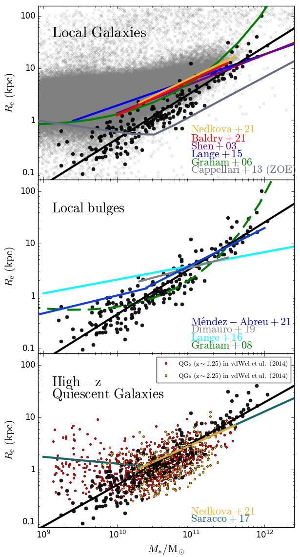
We further compare our spheroids to the galaxy and bulge size–mass relations in the literature. Fig. 15 shows a comparison of our spheroids with local galaxies (upper panel), local bulges/spheroids (middle panel), and high- quiescent galaxies (bottom panel). Our spheroid size-mass relation (solid black line) and data (black points) are plotted in all three panels.
In the upper panel of Fig. 13, the galaxy size-mass relation from the following works are shown: Shen et al. (2003), Graham et al. (2006), Lange et al. (2015), Baldry et al. (2021), Nedkova et al. (2021, their quiescent galaxies (QGs) at ). Additionally, the empirical zone of exclusion (ZOE, Bender et al., 1992; Burstein et al., 1997), defined in Cappellari et al. (2013a), is shown with a bent solid grey line. The grey cloud depicts the SDSS galaxies from the NASA-Sloan ATLAS catalogue at .
Our spheroid relation resides on the high-mass and small-radius side of the SDSS galaxies. It also presents a steeper slope () compared to the galaxy relations. Simply put, the spheroids are more compact than ETGs or QGs. At the high-mass end (), the galaxy size-mass relation from Shen et al. (2003), Lange et al. (2015), Baldry et al. (2021), and Nedkova et al. (2021, ) align better with our spheroid relation than compared to the low-mass end (). This is because single-component spheroidal E galaxies dominate the high-mass range. Our spheroids at the high-mass end are elliptical galaxies modelled with a single Sérsic function similar to the earlier works. E galaxies appear to follow the same continuous log-linear relation as the embedded spheroids in S0 and S galaxies. Indeed, Lange et al. (2016) show that their galaxy size-mass relation was the steepest () when they only considered massive galaxies (, see their Table 1), a result much closer to our relation. Further, the ZOE presented in Cappellari et al. (2013a) is an empirical model of a double-power law that cuddles the lower bound of their galaxy size-mass distribution. It depicts an empirical lower limit for galaxies’ size and maximum density. However, note that Cappellari et al. (2013a)’s ZOE is constructed with local galaxies (within ). The embedded spheroids need not conform to such a constraint. If indeed some spheroids are already fully formed at high-, the ZOE at higher could be different to the ZOE in Cappellari et al. (2013a). Since the spheroids’ relation roughly follows a log-linear trend across , its ZOE should also be log-linear.
4.3.2 Comparison with local bulges
Our result also highlights the necessity for multicomponent decomposition in order to extract bulges correctly. In the middle panel of Fig. 15, we compare our spheroids with some bulge size-mass relations at low-: Graham & Worley (2008), Lange et al. (2016), Dimauro et al. (2019), and Méndez-Abreu et al. (2021). Building on Allen et al. (2006), Lange et al. (2016) performed an automatic Bulge+Disc decomposition of 2247 ETGs and LTGs with stellar mass at taken from the Galaxy And Mass Assembly (GAMA) survey (GAMA II, Driver et al., 2009, 2016; Liske et al., 2015). They improved on the conventional fitting routines by performing multiple fits with a wide range of starting parameters and using the median value of these fits to obtain the size–mass relation. However, their bulge size-mass relations differ significantly from our spheroid relation, with the slope (Lange et al., 2016, see their Table 1). In Dimauro et al. (2019), the slope of the size–mass relation iss for all bulges coming from galaxies with at . Since both their methods do not account for potentially biasing components, e.g., bars, disc truncation and anti-trucation, and nuclear components, the bulge sizes are likely overestimated. On the contrary, Méndez-Abreu et al. (2017); Méndez-Abreu et al. (2021) present a bulge relation made using 2D multi-component decomposition for 404 galaxies at in the Calar Alto Legacy Integral Field Area survey (CALIFA-DR3, García-Benito et al., 2015; Sánchez et al., 2016) that includes a variety of components, specifically, the bulge, bar, nuclear point source, and Type I-III disc. As a result, their bulge size–mass relation is the closest to ours, with a slope of for bulges with . Interestingly, however, the low-mass () bulges in Méndez-Abreu et al. (2021) follows a shallower relation with a slope of , resulting in an ‘up-bend’ in the overall size–mass relation. Similar up-bend at – was also reported in other works (e.g., Gadotti, 2008; Laurikainen et al., 2010).
We note that the absent of up-bend in our relation could be a result of sample selection. From Fig. 8 in Laurikainen et al. (2010), we can see that bulges from Sc or later-type spiral (Sc-) galaxies dominate the low-mass range (–). Without the Sc- bulges, their spheroid size–luminosity distribution resembles a log-linear relation. Sc- galaxies are also abundant in the parent sample of the aforementioned work that presented the up-bend (Gadotti, 2009; Lange et al., 2016; Méndez-Abreu et al., 2021). However, since our data sources, H+22 and D+19, contain mostly early-type (Sa-Sb) spiral galaxies, the up-bend is not present in our spheroid size–mass relation. While our sample does not contain many late-type (Sc-Sd) spiral galaxies, or more specifically, galaxies with , the light-green curve in Fig. 9 suggests a possible flattening of the size-mass relation at low masses. Late-type spiral galaxies can, however, be challenging to model because they typically contain bulges whose surface brightness is relatively faint compared to the inner disc (Graham, 2001, their Fig. 21), and with ground-bases seeing, the bars of bulgeless spiral galaxies can mimic bulges (e.g. Baldassare et al., 2015, 2017). While our colleagues have addressed these issues and measured a reduction of the slope in the size-mass diagram for late-type spiral galaxies, we do not attempt to do this.
When the disc (and any additional inner-disc) and disc-induced components (e.g., bars and spiral arms) are removed, the remaining component would be the relatively dense spheroid. Galaxy size-mass relations possess a flatter slope than spheroids’ because the disc in S0 and S galaxies, which exist at lower-mass end, increases the overall size and decreases the overall density of a galaxy. The deviation between the galaxy and spheroid size-mass relation is more prominent at the low-mass end (), where the galaxies tend to have a lower bulge-to-total flux ratio and the disc’s mass trumps the spheroids’.
4.3.3 Comparison with high- quiescent galaxies
With the knowledge that ETGs have a different size-mass relation than the spheroids, kicking up in size at low-mass end because of the disc, we compare our spheroid relation with the quiescent galaxies at . The bottom panel of Fig. 15 shows the galaxy size-mass relation at : Nedkova et al. (2021, QGs at ) and Saracco et al. (2017, QGs at ). The red and orange points are the QGs from CANDELS (van der Wel et al., 2014) at and (their Fig. 5)222222The original size-mass distribution was depicted using the effective radius in the major-axis instead of the circularised radius. Following what was done in Saracco et al. (2017), we scaled down their radius by the average radius ratio (Cappellari et al., 2013b) to match the size-mass relations in the other studies., respectively. The relation in Nedkova et al. (2021) matches the high-mass () end of the relation in Saracco et al. (2017) remarkably well. Compared to the Nedkova et al. (2021) galaxy size-mass relation at (see the upper panel of Fig. 15), their relation at migrates toward the lower-right side of the plot, implying quiescent galaxies are more compact as redshift increases (see also van der Wel et al., 2014). The up-bend at in the Saracco et al. (2017) galaxy size-mass relation is also present in the QGs from van der Wel et al. (2014) at –. The QGs from van der Wel et al. (2014) at – follow a similar trend to our spheroids’ size-mass relation. In between , our spheroids reside in the middle of the van der Wel et al. (2014)’s QGs distribution. It shows that, in terms of size and mass, local spheroids are structurally similar to high- quiescent galaxies. The galaxy size evolution among QGs has been discussed by many studies (e.g., Trujillo et al., 2007; Bezanson et al., 2009; Taylor et al., 2010; Barro et al., 2013; van der Wel et al., 2014; van Dokkum et al., 2015), where QGs become less compact as decreases. Since local spheroids are analogous to the quiescent system at , our result supports the scenario where the system builds from the inside-out, either through the disc-cloaking process (Graham et al., 2015; Hon et al., 2022) to build up a disc within over an existing spheroid to become S0 or S galaxy (see also Costantin et al., 2020, 2022), or major mergers to become an elliptical galaxy (Graham & Sahu 2022, in Press).
5 Summary
In this paper, using the local bulge/spheroid data from multi-component decompositions in SG16, D+19, S+19, and H+22, we present the followings:
-
•
The distribution of the spheroids’ band absolute magnitude () against their structural parameters, namely the spheroid’s Sérsic index (), central surface brightness (), and effective radius () have been presented in Section 3.1.
-
•
The correlation strength among , , and are measured (Section 3.2).
-
•
The – and – relations, using the different scale radii , enclosing different fractions of the spheroid light, are presented in Section 3.3.1.
-
•
The spheroid mass () versus Sérsic index (), projected mass density (), and effective radius () relations are provided in Section 3.4.1. Their behaviour resembles that of the –, – and – relations, with similar correlation strength.
-
•
We charted the correlation strength () as a function of the fraction of light, , included within the scale radii for different parameter (, , , and ) pairings with the spheroid mass (Section 3.4.3). Among them, the – relations consistently have the highest correlation strength () across all . The Sérsic ‘shape function’ – relations have the second highest correlation across all , with and , while the strength of the – and – relations vary significantly with the choice of .
-
•
The local spheroid size ()–mass () relation is presented in Section 3.5.1. For the full sample, the bisector regression line is:
(19) with an intrinsic scatter of .
-
•
Four additional scaling relations: –, –, –, and – are presented in Section 3.5.2. We obtained the bisector lines:
(20) with an intrinsic scatter of ;
(21) with an intrinsic scatter of ;
(22) with an intrinsic scatter of ; and
(23) with an intrinsic scatter of . In each case, the scatter is measured in the vertical direction.
Here, we briefly summarise the findings in this paper:
-
1.
There is no clear boundary between spheroids embedded in S0 and S galaxies. They have a significant overlap in the size-mass diagram and other parameter planes, indicating a shared origin or, at the very least, governing formation physics among bulges (see Section 4.2).
-
2.
The spheroid radius () is the best predictor of its luminosity and stellar mass, regardless of the fraction of light, , used. The shape of the spheroid’s light profile () and ‘shape function’, , also correlate well with the spheroid mass, albeit it not as strong as . The surface brightness, , and the surface mass densisities, and , are weak predictors of the spheroid stellar mass because of their low correlation with , a result which is also subject to the light fraction .
-
3.
The spheroid size ()–mass () distribution exhibits a roughly log-linear relation at , contrary to the curved size–mass predicted in Graham et al. (2006) for ETGs and the double-power law from other works. Since the disc (and other) components are less dense than the bulge, S0 and S galaxies will have a larger size than a pure spheroid at the same mass, resulting in the upbend in the low-mass end where discs are more prominent.
-
4.
The spheroid central surface brightness ()–Sérsic index () relation shows a strong linear trend (Fig.2). As such, in log-space (–), the relation appears curved. This is in contrast to the linear scaling – relation presented in Khosroshahi et al. (2000a). If the ‘photometric plane’ is present in our sample, we speculate its surface will also be curved if using .
-
5.
Our spheroid size-mass relation is a factor of steeper than some reported bulge size-mass relation obtained via Bulge+Disc decomposition. Likely due to the lack of Sc or later-type spiral galaxies in our sample, we do not see the flattening of slope (i.e. an up-bend) in the low-mass end () that is common in other bulge size–mass relation in the literature. Finally, our spheroids’ relation aligns well with the quiescent galaxy size-mass relation at and in between . It indicates that local spheroids are structurally similar to the high- quiescent galaxies.
Acknowledgements
This research was supported under the Australian Research Council’s funding scheme DP17012923. This research has made use of the NASA/IPAC Extragalactic Database (NED), which is funded by the National Aeronautics and Space Administration and operated by the California Institute of Technology.
The project is made possible by using the following software packages: AstroPy (Astropy Collaboration et al., 2013, 2018), Cmasher (van der Velden, 2020), IRAF (Tody, 1986, 1993), ISOFIT (Ciambur, 2015), Matplotlib (Hunter, 2007), NumPy (Harris et al., 2020), Profiler (Ciambur, 2016), SAOImageDS9 (Joye & Mandel, 2003), SciPy (Virtanen et al., 2020), SExtractor (Bertin & Arnouts, 1996), and TOPCAT (Taylor, 2005).
All the scripts used in the analysis are available on GitHub (https://github.com/dex-hon-sci/GalSpheroids).
Data Availability
The data underlying this article will be shared upon request to the corresponding author.
References
- Aguerri et al. (1998) Aguerri J. A. L., Beckman J. E., Prieto M., 1998, AJ, 116, 2136
- Aihara et al. (2011) Aihara H., et al., 2011, ApJS, 193, 29
- Allen et al. (2006) Allen P. D., Driver S. P., Graham A. W., Cameron E., Liske J., de Propris R., 2006, MNRAS, 371, 2
- Andredakis et al. (1995) Andredakis Y. C., Peletier R. F., Balcells M., 1995, MNRAS, 275, 874
- Aragón-Salamanca et al. (2006) Aragón-Salamanca A., Bedregal A. G., Merrifield M. R., 2006, A&A, 458, 101
- Astropy Collaboration et al. (2013) Astropy Collaboration et al., 2013, A&A, 558, A33
- Astropy Collaboration et al. (2018) Astropy Collaboration et al., 2018, AJ, 156, 123
- Balcells & Peletier (1994) Balcells M., Peletier R. F., 1994, AJ, 107, 135
- Balcells et al. (2007) Balcells M., Graham A. W., Peletier R. F., 2007, ApJ, 665, 1084
- Baldassare et al. (2015) Baldassare V. F., Reines A. E., Gallo E., Greene J. E., 2015, ApJ, 809, L14
- Baldassare et al. (2017) Baldassare V. F., Reines A. E., Gallo E., Greene J. E., 2017, ApJ, 850, 196
- Baldry et al. (2012) Baldry I. K., et al., 2012, MNRAS, 421, 621
- Baldry et al. (2021) Baldry I. K., Sullivan T., Rani R., Turner S., 2021, MNRAS, 500, 1557
- Barbosa et al. (2021) Barbosa C. E., Spiniello C., Arnaboldi M., Coccato L., Hilker M., Richtler T., 2021, A&A, 649, A93
- Barro et al. (2013) Barro G., et al., 2013, ApJ, 765, 104
- Barro et al. (2017) Barro G., et al., 2017, ApJ, 840, 47
- Barway et al. (2005) Barway S., Mayya Y. D., Kembhavi A. K., Pandey S. K., 2005, AJ, 129, 630
- Barway et al. (2009) Barway S., Wadadekar Y., Kembhavi A. K., Mayya Y. D., 2009, MNRAS, 394, 1991
- Begelman et al. (1980) Begelman M. C., Blandford R. D., Rees M. J., 1980, Nature, 287, 307
- Bellstedt et al. (2017) Bellstedt S., Forbes D. A., Foster C., Romanowsky A. J., Brodie J. P., Pastorello N., Alabi A., Villaume A., 2017, MNRAS, 467, 4540
- Bender et al. (1992) Bender R., Burstein D., Faber S. M., 1992, ApJ, 399, 462
- Bertin & Arnouts (1996) Bertin E., Arnouts S., 1996, A&AS, 117, 393
- Bezanson et al. (2009) Bezanson R., van Dokkum P. G., Tal T., Marchesini D., Kriek M., Franx M., Coppi P., 2009, ApJ, 697, 1290
- Binggeli & Jerjen (1998) Binggeli B., Jerjen H., 1998, A&A, 333, 17
- Bruzual & Charlot (2003) Bruzual G., Charlot S., 2003, MNRAS, 344, 1000
- Burstein et al. (1997) Burstein D., Bender R., Faber S., Nolthenius R., 1997, AJ, 114, 1365
- Buta & Combes (1996) Buta R., Combes F., 1996, Fundamentals Cosmic Phys., 17, 95
- Buta & Crocker (1993) Buta R., Crocker D. A., 1993, AJ, 105, 1344
- Byun et al. (1996) Byun Y. I., et al., 1996, AJ, 111, 1889
- Caon et al. (1993) Caon N., Capaccioli M., D’Onofrio M., 1993, MNRAS, 265, 1013
- Capaccioli et al. (1989) Capaccioli M., Della Valle M., D’Onofrio M., Rosino L., 1989, AJ, 97, 1622
- Cappellari et al. (2011a) Cappellari M., et al., 2011a, MNRAS, 413, 813
- Cappellari et al. (2011b) Cappellari M., et al., 2011b, MNRAS, 416, 1680
- Cappellari et al. (2013a) Cappellari M., et al., 2013a, MNRAS, 432, 1862
- Cappellari et al. (2013b) Cappellari M., et al., 2013b, MNRAS, 432, 1862
- Chabrier (2003) Chabrier G., 2003, PASP, 115, 763
- Ciambur (2015) Ciambur B. C., 2015, ApJ, 810, 120
- Ciambur (2016) Ciambur B. C., 2016, Publ. Astron. Soc. Australia, 33, e062
- Costantin et al. (2020) Costantin L., et al., 2020, ApJ, 889, L3
- Costantin et al. (2022) Costantin L., et al., 2022, ApJ, 929, 121
- D’Onofrio (2001) D’Onofrio M., 2001, MNRAS, 326, 1517
- D’Onofrio et al. (1994) D’Onofrio M., Capaccioli M., Caon N., 1994, MNRAS, 271, 523
- Davis et al. (2017) Davis B. L., Graham A. W., Seigar M. S., 2017, MNRAS, 471, 2187
- Davis et al. (2019) Davis B. L., Graham A. W., Cameron E., 2019, ApJ, 873, 85
- De Propris et al. (2005) De Propris R., Colless M., Driver S. P., Pracy M. B., Couch W. J., 2005, MNRAS, 357, 590
- De Propris et al. (2007) De Propris R., Conselice C. J., Liske J., Driver S. P., Patton D. R., Graham A. W., Allen P. D., 2007, ApJ, 666, 212
- De Propris et al. (2010) De Propris R., et al., 2010, AJ, 139, 794
- Dekel et al. (2019) Dekel A., Lapiner S., Dubois Y., 2019, arXiv e-prints, p. arXiv:1904.08431
- Dimauro et al. (2019) Dimauro P., et al., 2019, MNRAS, 489, 4135
- Driver et al. (2009) Driver S. P., et al., 2009, Astronomy and Geophysics, 50, 5.12
- Driver et al. (2013) Driver S. P., Robotham A. S. G., Bland-Hawthorn J., Brown M., Hopkins A., Liske J., Phillipps S., Wilkins S., 2013, MNRAS, 430, 2622
- Driver et al. (2016) Driver S. P., et al., 2016, MNRAS, 455, 3911
- Eisenhauer et al. (2011) Eisenhauer F., et al., 2011, The Messenger, 143, 16
- Erwin et al. (2003) Erwin P., Beltrán J. C. V., Graham A. W., Beckman J. E., 2003, ApJ, 597, 929
- Fazio et al. (2004) Fazio G. G., et al., 2004, ApJS, 154, 10
- Ferrarese et al. (1994) Ferrarese L., van den Bosch F. C., Ford H. C., Jaffe W., O’Connell R. W., 1994, AJ, 108, 1598
- Ferrarese et al. (2006) Ferrarese L., et al., 2006, ApJS, 164, 334
- Ferrers (1877) Ferrers N., 1877, QJ Pure Appl. Math, 14, 1
- Fisher & Drory (2010) Fisher D. B., Drory N., 2010, ApJ, 716, 942
- Forbes et al. (2008) Forbes D. A., Lasky P., Graham A. W., Spitler L., 2008, MNRAS, 389, 1924
- Fukugita et al. (1996) Fukugita M., Ichikawa T., Gunn J. E., Doi M., Shimasaku K., Schneider D. P., 1996, AJ, 111, 1748
- Gadotti (2008) Gadotti D. A., 2008, MNRAS, 384, 420
- Gadotti (2009) Gadotti D. A., 2009, MNRAS, 393, 1531
- García-Benito et al. (2015) García-Benito R., et al., 2015, A&A, 576, A135
- Gillessen et al. (2010) Gillessen S., et al., 2010, in Danchi W. C., Delplancke F., Rajagopal J. K., eds, Society of Photo-Optical Instrumentation Engineers (SPIE) Conference Series Vol. 7734, Optical and Infrared Interferometry II. p. 77340Y (arXiv:1007.1612), doi:10.1117/12.856689
- Graham (2001) Graham A. W., 2001, AJ, 121, 820
- Graham (2013) Graham A. W., 2013, Elliptical and Disk Galaxy Structure and Modern Scaling Laws. Springer Science+Business Media Dordrecht, pp 91–140, doi:10.1007/978-94-007-5609-0_2
- Graham (2019a) Graham A. W., 2019a, Publ. Astron. Soc. Australia, 36, e035
- Graham (2019b) Graham A. W., 2019b, MNRAS, 487, 4995
- Graham & Driver (2005) Graham A. W., Driver S. P., 2005, Publ. Astron. Soc. Australia, 22, 118
- Graham & Guzmán (2003) Graham A. W., Guzmán R., 2003, AJ, 125, 2936
- Graham & Scott (2013) Graham A. W., Scott N., 2013, ApJ, 764, 151
- Graham & Worley (2008) Graham A. W., Worley C. C., 2008, MNRAS, 388, 1708
- Graham et al. (1996) Graham A., Lauer T. R., Colless M., Postman M., 1996, ApJ, 465, 534
- Graham et al. (2003a) Graham A. W., Erwin P., Trujillo I., Asensio Ramos A., 2003a, AJ, 125, 2951
- Graham et al. (2003b) Graham A. W., Jerjen H., Guzmán R., 2003b, AJ, 126, 1787
- Graham et al. (2006) Graham A. W., Merritt D., Moore B., Diemand J., Terzić B., 2006, AJ, 132, 2711
- Graham et al. (2015) Graham A. W., Dullo B. T., Savorgnan G. A. D., 2015, ApJ, 804, 32
- Graham et al. (2016) Graham A. W., Ciambur B. C., Savorgnan G. A. D., 2016, ApJ, 831, 132
- Graham et al. (2017) Graham A. W., Janz J., Penny S. J., Chilingarian I. V., Ciambur B. C., Forbes D. A., Davies R. L., 2017, ApJ, 840, 68
- Greenhill et al. (2003) Greenhill L. J., et al., 2003, ApJ, 590, 162
- Harris et al. (2020) Harris C. R., et al., 2020, Nature, 585, 357
- Heidmann (1969) Heidmann J., 1969, Astrophys. Lett., 3, 19
- Holmberg (1969) Holmberg E., 1969, Arkiv for Astronomi, 5, 305
- Hon et al. (2022) Hon D. S. H., Graham A. W., Davis B. L., Marconi A., 2022, MNRAS, 514, 3410
- Hopkins et al. (2009) Hopkins P. F., Bundy K., Murray N., Quataert E., Lauer T. R., Ma C.-P., 2009, MNRAS, 398, 898
- Hunter (2007) Hunter J. D., 2007, Computing in Science & Engineering, 9, 90
- Iodice et al. (1999) Iodice E., D’Onofrio M., Capaccioli M., 1999, in Giuricin G., Mezzetti M., Salucci P., eds, Astronomical Society of the Pacific Conference Series Vol. 176, Observational Cosmology: The Development of Galaxy Systems. p. 402
- Jablonka et al. (2007) Jablonka P., Gorgas J., Goudfrooij P., 2007, A&A, 474, 763
- Janz et al. (2014) Janz J., et al., 2014, ApJ, 786, 105
- Jarrett et al. (2003) Jarrett T. H., Chester T., Cutri R., Schneider S. E., Huchra J. P., 2003, AJ, 125, 525
- Joye & Mandel (2003) Joye W. A., Mandel E., 2003, in Payne H. E., Jedrzejewski R. I., Hook R. N., eds, Astronomical Society of the Pacific Conference Series Vol. 295, Astronomical Data Analysis Software and Systems XII. p. 489
- Jungwiert et al. (1997) Jungwiert B., Combes F., Axon D. J., 1997, A&AS, 125, 479
- Kelly (2007) Kelly B. C., 2007, ApJ, 665, 1489
- Kelvin et al. (2012) Kelvin L. S., et al., 2012, MNRAS, 421, 1007
- Kennedy et al. (2016) Kennedy R., Bamford S. P., Häußler B., Brough S., Holwerda B., Hopkins A. M., Vika M., Vulcani B., 2016, A&A, 593, A84
- Khosroshahi et al. (2000a) Khosroshahi H. G., Wadadekar Y., Kembhavi A., Mobasher B., 2000a, ApJ, 531, L103
- Khosroshahi et al. (2000b) Khosroshahi H. G., Wadadekar Y., Kembhavi A., 2000b, ApJ, 533, 162
- King (1978) King I. R., 1978, ApJ, 222, 1
- Kormendy & Bender (2012) Kormendy J., Bender R., 2012, ApJS, 198, 2
- Kormendy & Freeman (2016) Kormendy J., Freeman K. C., 2016, ApJ, 817, 84
- Kormendy et al. (2009) Kormendy J., Fisher D. B., Cornell M. E., Bender R., 2009, ApJS, 182, 216
- Lange et al. (2015) Lange R., et al., 2015, MNRAS, 447, 2603
- Lange et al. (2016) Lange R., et al., 2016, MNRAS, 462, 1470
- Larson (1976) Larson R. B., 1976, MNRAS, 176, 31
- Läsker et al. (2014) Läsker R., Ferrarese L., van de Ven G., 2014, ApJ, 780, 69
- Laurikainen et al. (2005) Laurikainen E., Salo H., Buta R., 2005, MNRAS, 362, 1319
- Laurikainen et al. (2010) Laurikainen E., Salo H., Buta R., Knapen J. H., Comerón S., 2010, MNRAS, 405, 1089
- Le Bouquin et al. (2011) Le Bouquin J. B., et al., 2011, A&A, 535, A67
- Liller (1966) Liller M. H., 1966, ApJ, 146, 28
- Liske et al. (2015) Liske J., et al., 2015, MNRAS, 452, 2087
- MacArthur et al. (2008) MacArthur L. A., Ellis R. S., Treu T., U V., Bundy K., Moran S., 2008, ApJ, 680, 70
- MacArthur et al. (2009) MacArthur L. A., González J. J., Courteau S., 2009, MNRAS, 395, 28
- Martin (1995) Martin P., 1995, AJ, 109, 2428
- Martinez-Valpuesta et al. (2007) Martinez-Valpuesta I., Knapen J. H., Buta R., 2007, AJ, 134, 1863
- McDermid et al. (2020) McDermid R., et al., 2020, Phase A Science Case for MAVIS – The Multi-conjugate Adaptive-optics Visible Imager-Spectrograph for the VLT Adaptive Optics Facility. Macquarie University, doi:10.25949/zdaw-rx65
- Meidt et al. (2014) Meidt S. E., et al., 2014, ApJ, 788, 144
- Méndez-Abreu et al. (2017) Méndez-Abreu J., et al., 2017, A&A, 598, A32
- Méndez-Abreu et al. (2021) Méndez-Abreu J., de Lorenzo-Cáceres A., Sánchez S. F., 2021, MNRAS, 504, 3058
- Möllenhoff & Heidt (2001) Möllenhoff C., Heidt J., 2001, A&A, 368, 16
- Moorthy & Holtzman (2006) Moorthy B. K., Holtzman J. A., 2006, MNRAS, 371, 583
- Morishita et al. (2017) Morishita T., et al., 2017, ApJ, 835, 254
- Naab et al. (2009) Naab T., Johansson P. H., Ostriker J. P., 2009, ApJ, 699, L178
- Nair et al. (2011) Nair P., van den Bergh S., Abraham R. G., 2011, ApJ, 734, L31
- Nedkova et al. (2021) Nedkova K. V., et al., 2021, MNRAS, 506, 928
- Ni et al. (2021) Ni Q., et al., 2021, MNRAS, 500, 4989
- Nilson (1973) Nilson P., 1973, Uppsala general catalogue of galaxies
- Noordeh et al. (2021) Noordeh E., Canning R. E. A., Willis J. P., Allen S. W., Mantz A., Stanford S. A., Brammer G., 2021, MNRAS, 507, 5272
- Oemler (1976) Oemler A. J., 1976, ApJ, 209, 693
- Patterson (1940) Patterson F. S., 1940, Harvard College Observatory Bulletin, 914, 9
- Pohlen et al. (2002) Pohlen M., Dettmar R. J., Lütticke R., Aronica G., 2002, A&A, 392, 807
- Prieto et al. (1997) Prieto M., Gottesman S. T., Aguerri J.-A. L., Varela A.-M., 1997, AJ, 114, 1413
- Proctor & Sansom (2002) Proctor R. N., Sansom A. E., 2002, MNRAS, 333, 517
- Querejeta et al. (2015) Querejeta M., et al., 2015, ApJS, 219, 5
- Rigaut et al. (2020) Rigaut F., et al., 2020, in Society of Photo-Optical Instrumentation Engineers (SPIE) Conference Series. p. 114471R, doi:10.1117/12.2561886
- Rizzo et al. (2018) Rizzo F., Fraternali F., Iorio G., 2018, MNRAS, 476, 2137
- Roediger & Courteau (2015) Roediger J. C., Courteau S., 2015, MNRAS, 452, 3209
- Romanowsky & Fall (2012) Romanowsky A. J., Fall S. M., 2012, ApJS, 203, 17
- Rusli et al. (2013) Rusli S. P., Erwin P., Saglia R. P., Thomas J., Fabricius M., Bender R., Nowak N., 2013, AJ, 146, 160
- Sahu et al. (2019) Sahu N., Graham A. W., Davis B. L., 2019, ApJ, 876, 155
- Sahu et al. (2020) Sahu N., Graham A. W., Davis B. L., 2020, ApJ, 903, 97
- Sahu et al. (2022) Sahu N., Graham A. W., Davis B. L., 2022, ApJ, 927, 67
- Sánchez et al. (2016) Sánchez S. F., et al., 2016, A&A, 594, A36
- Sandage & Tammann (1981) Sandage A., Tammann G. A., 1981, A Revised Shapley-Ames Catalog of Bright Galaxies
- Saracco et al. (2009) Saracco P., Longhetti M., Andreon S., 2009, MNRAS, 392, 718
- Saracco et al. (2017) Saracco P., Gargiulo A., Ciocca F., Marchesini D., 2017, A&A, 597, A122
- Saslaw et al. (1974) Saslaw W. C., Valtonen M. J., Aarseth S. J., 1974, ApJ, 190, 253
- Savorgnan & Graham (2016a) Savorgnan G. A. D., Graham A. W., 2016a, ApJS, 222, 10
- Savorgnan & Graham (2016b) Savorgnan G. A. D., Graham A. W., 2016b, MNRAS, 457, 320
- Savorgnan et al. (2013) Savorgnan G., Graham A. W., Marconi A., Sani E., Hunt L. K., Vika M., Driver S. P., 2013, MNRAS, 434, 387
- Savorgnan et al. (2016) Savorgnan G. A. D., Graham A. W., Marconi A. r., Sani E., 2016, ApJ, 817, 21
- Scorza & van den Bosch (1998) Scorza C., van den Bosch F. C., 1998, MNRAS, 300, 469
- Scott et al. (2015) Scott N., et al., 2015, MNRAS, 451, 2723
- Seigar & James (1998) Seigar M. S., James P. A., 1998, MNRAS, 299, 672
- Sellwood & Wilkinson (1993) Sellwood J. A., Wilkinson A., 1993, Reports on Progress in Physics, 56, 173
- Sérsic (1968) Sérsic J. L., 1968, Atlas de Galaxias Australes. Cordoba Observatorio Astronomico, Cordoba, Argentina
- Shaw et al. (1993) Shaw M. A., Combes F., Axon D. J., Wright G. S., 1993, A&A, 273, 31
- Shen et al. (2003) Shen S., Mo H. J., White S. D. M., Blanton M. R., Kauffmann G., Voges W., Brinkmann J., Csabai I., 2003, MNRAS, 343, 978
- Sheth et al. (2010) Sheth K., et al., 2010, PASP, 122, 1397
- Simard et al. (2002) Simard L., et al., 2002, ApJS, 142, 1
- Simard et al. (2011) Simard L., Mendel J. T., Patton D. R., Ellison S. L., McConnachie A. W., 2011, ApJS, 196, 11
- Somerville & Davé (2015) Somerville R. S., Davé R., 2015, ARA&A, 53, 51
- Stiavelli et al. (2001) Stiavelli M., Miller B. W., Ferguson H. C., Mack J., Whitmore B. C., Lotz J. M., 2001, AJ, 121, 1385
- Strom & Strom (1978) Strom S. E., Strom K. M., 1978, AJ, 83, 732
- Taylor (2005) Taylor M. B., 2005, in Shopbell P., Britton M., Ebert R., eds, Astronomical Society of the Pacific Conference Series Vol. 347, Astronomical Data Analysis Software and Systems XIV. p. 29
- Taylor et al. (2010) Taylor E. N., Franx M., Glazebrook K., Brinchmann J., van der Wel A., van Dokkum P. G., 2010, ApJ, 720, 723
- Thomas & Davies (2006) Thomas D., Davies R. L., 2006, MNRAS, 366, 510
- Tinsley & Larson (1978) Tinsley B. M., Larson R. B., 1978, ApJ, 221, 554
- Tody (1986) Tody D., 1986, in Crawford D. L., ed., Society of Photo-Optical Instrumentation Engineers (SPIE) Conference Series Vol. 627, Instrumentation in astronomy VI. p. 733, doi:10.1117/12.968154
- Tody (1993) Tody D., 1993, in Hanisch R. J., Brissenden R. J. V., Barnes J., eds, Astronomical Society of the Pacific Conference Series Vol. 52, Astronomical Data Analysis Software and Systems II. p. 173
- Tolstoy et al. (2009) Tolstoy E., Hill V., Tosi M., 2009, ARA&A, 47, 371
- Trujillo et al. (2004) Trujillo I., Erwin P., Asensio Ramos A., Graham A. W., 2004, AJ, 127, 1917
- Trujillo et al. (2007) Trujillo I., Conselice C. J., Bundy K., Cooper M. C., Eisenhardt P., Ellis R. S., 2007, MNRAS, 382, 109
- Trujillo et al. (2011) Trujillo I., Ferreras I., de La Rosa I. G., 2011, MNRAS, 415, 3903
- Vika et al. (2012) Vika M., Driver S. P., Cameron E., Kelvin L., Robotham A., 2012, MNRAS, 419, 2264
- Virtanen et al. (2020) Virtanen P., et al., 2020, Nature Methods, 17, 261
- Vulcani et al. (2014) Vulcani B., et al., 2014, MNRAS, 441, 1340
- Watkins et al. (2022) Watkins A. E., et al., 2022, arXiv e-prints, p. arXiv:2201.08381
- Werner et al. (2004) Werner M. W., et al., 2004, ApJS, 154, 1
- Williams et al. (2010) Williams M. J., Bureau M., Cappellari M., 2010, MNRAS, 409, 1330
- Wozniak et al. (1995) Wozniak H., Friedli D., Martinet L., Martin P., Bratschi P., 1995, A&AS, 111, 115
- York et al. (2000) York D. G., et al., 2000, AJ, 120, 1579
- Young & Currie (1994) Young C. K., Currie M. J., 1994, MNRAS, 268, L11
- de Grijs et al. (2001) de Grijs R., Kregel M., Wesson K. H., 2001, MNRAS, 324, 1074
- de Vaucouleurs (1948) de Vaucouleurs G., 1948, Annales d’Astrophysique, 11, 247
- de Vaucouleurs (1957) de Vaucouleurs G., 1957, AJ, 62, 69
- de Vaucouleurs et al. (1991) de Vaucouleurs G., de Vaucouleurs A., Corwin Herold G. J., Buta R. J., Paturel G., Fouque P., 1991, Third Reference Catalogue of Bright Galaxies. Springer, New York, NY, USA
- van Dokkum et al. (2015) van Dokkum P. G., et al., 2015, ApJ, 813, 23
- van den Bergh (2008) van den Bergh S., 2008, A&A, 490, 97
- van den Bergh (2009) van den Bergh S., 2009, ApJ, 694, L120
- van den Bosch (1998) van den Bosch F. C., 1998, ApJ, 507, 601
- van der Kruit & Searle (1981) van der Kruit P. C., Searle L., 1981, A&A, 95, 116
- van der Velden (2020) van der Velden E., 2020, The Journal of Open Source Software, 5, 2004
- van der Wel et al. (2014) van der Wel A., et al., 2014, ApJ, 788, 28