The Shadow Knows: Empirical Distributions of Minimum Spanning Acycles and Persistence Diagrams of Random Complexes
Abstract
In 1985, Frieze showed that the expected sum of the edge weights of the minimum spanning tree (MST) in the uniformly weighted graph converges to . Recently, Hino and Kanazawa extended this result to a uniformly weighted simplicial complex, where the role of the MST is played by its higher-dimensional analog—the Minimum Spanning Acycle (MSA). Our work goes beyond and describes the histogram of all the weights in this random MST and random MSA. Specifically, we show that their empirical distributions converge to a measure based on a concept called the shadow. The shadow of a graph is the set of all the missing transitive edges and, for a simplicial complex, it is a related topological generalization. As a corollary, we obtain a similar claim for the death times in the persistence diagram corresponding to the above weighted complex, a result of interest in applied topology.
title = The Shadow knows: Empirical Distributions of Minimum Spanning Acycles and Persistence Diagrams of Random Complexes, author = Nicolas Fraiman, Sayan Mukherjee, and Gugan Thoppe, plaintextauthor = Nicolas Fraiman, Sayan Mukherjee, and Gugan Thoppe, runningtitle = Empirical Distributions of Minimum Spanning Acycles and Persistence Diagrams, runningauthor = Nicolas Fraiman, Sayan Mukherjee, and Gugan Thoppe, copyrightauthor = Nicolas Fraiman, Sayan Mukherjee, and Gugan Thoppe, keywords = minimum spanning tree, minimum spanning acycle, persistence diagram, shadow, empirical measure, random graph, random complex, histogram, \dajEDITORdetailsyear=2023, number=2, received=13 January 2021, published=3 May 2023, doi=10.19086/da.73323,
[classification=text]
1 Introduction
Random graphs, as models for binary relations, deeply impact discrete mathematics, computer science, engineering, and statistics. However, modern-day data analysis also involves studying models with higher-order relations such as random simplicial complexes [13]. Our contributions here are vital from both these perspectives. Specifically, we consider a mean-field model for random graphs and random simplicial complexes and provide a complete description of the distribution of weights in the Minimum Spanning Tree (MST) and its higher dimensional analog—the Minimum Spanning Acycle (MSA). As a corollary, we also obtain the distribution of the death times in the associated persistence diagram.
To help judge our contributions, we refer the reader to Robert Adler’s 2014 article [1]. There he summed up the state-of-the-art in random topology as follows: while a lot is known about the asymptotic behaviors of the sums of MST and MSA weights and also their associated death times, almost nothing is known about the individual values. The work in [12] addressed this gap partially. There, the distributions of the extremal MSA weights and the extremal death times were studied. In this work, we go beyond and describe the behavior in the bulk. We emphasize that our result is new, even in the graph case.
1.1 Overview of Key Contributions
We now provide a summary of our main result along with its visual illustration. The necessary background is given in parallel.
A simplicial complex on a vertex set is a collection of subsets of that is closed under the subset operation. Trivially, every graph is a simplicial complex. However, the closure is what distinguishes a simplicial complex from a hypergraph, the other standard model for studying higher-order relations. In particular, all simplicial complexes are hypergraphs, but the reverse is not true. We refer to an element of with cardinality as a -dimensional face or simply a -face. Similarly, the -skeleton of denoted refers to the subset of faces with dimension less than or equal to
Let and be the weighted simplicial complex, where i.) is the complete -skeleton on vertices, i.e., is the set of all subsets that have cardinality less than or equal to and ii.) is a weight function such that is an independent uniform random variable if is a -face, and zero otherwise. Let be a -dimensional MSA111We provide the formal definition of an MSA in Section 2, but the reader unfamiliar with this term can set and replace MSA with a MST to read ahead. (or -MSA in short) in Then our main result can be informally stated as follows (see Section 2 for the details).
Theorem.
(Informal summary of our Main Result) As the empirical measure related to converges to a deterministic measure related to the asymptotic shadow density of the -dimensional Linial-Meshulam complex see (6) for the exact definition of
Intuitively, our result says that the normalized count of the face weights—after being scaled by —that lie in any subset of the real line asymptotically converges to that subset’s measure under The next couple of paragraphs briefly explain what this measure is.
Recall that the Erdős-Rényi graph, denoted by is a random graph on vertices where each edge is present with probability independently. The -dimensional Linial-Meshulam complex or simply is an analog of this model in higher dimensions. This random complex has vertices and the complete -skeleton; further, the -faces are included with probability independently. It is easy to see that and are equivalent.
The shadow of a graph is the set of all the missing transitive edges. That is, it includes a vertex pair if ’s edge set excludes such a pair, but contains an alternative path from to via other edges. Clearly, each vertex pair in ’s shadow has endpoints in any one component of A simplicial complex’s shadow is a related topological generalization; see Definition 3 for details.
The shadow of the random complex was investigated in [10], and its cardinality, after a suitable normalization, was shown to converge to a deterministic constant Now, is that measure whose density is, loosely, one minus the function made up of these constants for different values.


Figure 1 illustrates our main result pictorially. The two scenarios shown there correspond to two different values of the pair The yellow plots show the normalized histogram of the set while the red curves show the density of the shadow based limiting measure Observe that the red curves and the top of the yellow plots more or less resemble each other. Our main result loosely states that the difference between them decays to zero, as
The weighted simplicial complex can also be viewed as the evolving simplicial complex where In this evolution, monotically grows from a simplicial complex with an (almost surely) empty -skeleton (when ) to one that has all the -faces (when ). There is a natural persistence diagram associated with this process, which records the birth and death times of the different topological holes that appear and disappear as the process evolves. In [12, Theorem 3], it was shown that the set of death times in the -th dimension of this diagram exactly equals the set of weights in the -MSA of Consequently, the above result can also be stated in terms of the death times in the persistence diagram related to
1.2 Related Work
Our work lies at the intersection of two broad strands of research: one concerning component sizes, shadow densities, and homologies of random graphs and random complexes, and the other dealing with the statistics of weights in random MSTs and MSAs. In this section, we look at a few of the historical milestones in these two strands.
Erdős and Rényi were the ones who initiated the first strand with their work in [2]. There they showed that is a sharp asymptotic threshold for connectivity in Also that, if for and then i.) almost all the vertices in lie in one single component, and ii.) the vertices outside this are all isolated and their number has a Poisson distribution with mean This result was subsequently refined in [3] and the new statement included the following additional facts: i.) the asymptotic order of the largest component jumps from logarithmic to linear around and ii.) for the largest component in denoted satisfies where denotes the cardinality of a set and is the unique root in of the equation
| (1) |
A graph is a one-dimensional simplicial complex, so one can ask if phenomena like the ones above also occur in random complexes. Since connectivity is related to the vanishing of the zeroth homology, it is natural to look at the higher order Betti numbers to answer this question. Such a study was done in [8, 11], and it was found that the -th Betti number of indeed shows a non-vanishing to vanishing phase transition at A separate study [6] also showed that this Betti number converges to a Poisson random variable with mean when for
The result on component sizes, in contrast, was not so easy to generalize. The challenge was in coming up with a higher dimensional analog of a component in a simplicial complex. The breakthrough came in [9] with the introduction of the shadow. The underlying motivation was that, in a sparse graph, a giant component exists if and only if the shadow includes a positive fraction of all the possible edges. With this in mind, the behavior of the -dimensional shadow (or -shadow) of was investigated in [10], and these were the key findings there. One, changes from to at where equals when but is strictly greater than for Two, for where is the smallest root in of the equation
| (2) |
The pioneering work in the second strand was done by Frieze [4]. He showed that, given a complete graph on vertices with uniform weights on each edge, the expected sum of weights in the MST converges to the constant as Note that this graph is the case of our model. Recently, [5] showed that a similar result exists even for the -MSA of for


Separately, [12] studied the extremal weights in the -MSA of An illustration of a main result there is given in Figure 2. It shows two distinct scenarios. In both, a plot of the values in is given. This choice of scaling gives more prominence to the extremal weights, which in the two plots are the values on the extreme right. The result in [12] states that these extremal values converge to a Poisson point process, while the rest go to
1.3 Proof Outline
We now briefly describe how we combine the different facts stated above for proving our main result. Let be an arbitrary -face in and suppose Let Clearly, the distributions of and ), and hence of their shadows, are identical. Now, [12, Lemma 32] states that belongs to the -MSA of if and only if it does not lie in the shadow222The word ‘shadow’ is not used in [12], but the result can be interpreted in terms of the shadow in a straightforward fashion. of Given that could potentially have been any of the -faces outside of the probability that it belongs to the -MSA must then equal one minus the shadow density of By shadow density, we mean the shadow’s size divided by the total number of potential -faces. Based on this and the shadow density results from [10], the desired result is then easy to see.
2 Main Result
We give our main result here along with all the definitions that were skipped in Section 1. All the while, we presume that the reader is well versed with the basics of simplicial homology. If not, the necessary background can be found in [12, Section 2] and the references therein.
For a simplicial complex we use and to denote the set of -faces and the -th reduced Betti number333Throughout we assume the Betti numbers are defined using real coefficients, as in [10]., respectively. We drop from these notations, when the underlying simplicial complex is clear. Separately, for a random variable we use to represent its -th norm.
Our first aim is to define spanning acycles [7] and MSAs, the main objects of our study. These are topological generalizations of spanning trees and MSTs, respectively. Recall that a spanning tree in a connected graph is a subset of edges that connects all the vertices together without creating any cycles. In that same spirit, a -spanning acycle in a simplicial complex is a subset of -faces which when added to i.e., the -skeleton of kills the -th Betti number of but does not create any new -cycles. Finally, a MSA in a weighted simplicial complex is simply the spanning acycle with the smallest possible weight. As shown in [12, Lemma 23], a spanning acycle and, hence, a -MSA exists in if and only if
Definition 1 (Spanning Acycle).
Let be a simplicial complex with . Then, a -spanning acycle of is a set of -faces in such that .
Definition 2 (Minimum Spanning Acycle).
Let be a weighted -complex with . Then, a -MSA of is an element of , where the minimum is taken over all the -spanning acycles and represents the sum of weights of the faces in .
We remark that an MSA is unique when the -faces in have unique weights, e.g., see [12].
Next, we discuss the concept of a shadow. Introduced in [9], the shadow of a graph is the set of all those missing edges which when added will create a cycle. A simplicial complex’s shadow is the topological generalization of this concept. To state the formal definition, we need the notion of the dimension of a simplicial complex. This is the largest for which
Definition 3 (Shadow).
For a -dimensional simplicial complex with vertex set and having the complete -skeleton, its -shadow is given by
where denotes the set of all -sized subsets of
In analogy with the terms for the spectrum of random matrices, we next define the empirical measures that we study in this work. Let be the set of death times in the -th persistence diagram of the evolving simplicial complex associated with Also, let be the Dirac measure.
Definition 4 (Empirical Measure).
The empirical measures corresponding to the face weights in and the death times in are the random measures respectively given by
| (3) |
Finally, we define the deterministic measure which serves as the limit for both and Let be the smallest root in of the equation
| (4) |
It can be checked that for and is for Next, let where for That is, let
| (5) |
Now, for let be as in Section 1.2, i.e., the smallest root in of (2). Clearly, i.e., for any Building upon these terms, let be the measure whose density is given by
| (6) |
where
| (7) |
We remark that this is the same constant that we came across in Section 1.3. Separately, it follows from [10, Theorem 1.4] that for represents the asymptotic density of the shadow of i.e.,
We now state our main result. Define to be the Kolmogorov metric between the two measures and , i.e., let
Theorem 1 (Main Result).
Let . Then the random measures and converge in the Kolmogorov metric to in . Moreover, if is a continuous function with and
| (8) |
then both and converge to in .
Corollary 2.
Remark 3.
In Section 4, we discuss three extensions of the above result. The first two relate to the cases where the -face weights have a generic distribution and an additional noisy perturbation. The third one is about the weighted complex, wherein not all the potential -faces may be present.
Remark 4.
Theorem 1 readily applies when is bounded since hypothesis (8) is then trivially satisfied. Hence, an immediate consequence of our result is that converges to weakly in . However, our result also applies to unbounded functions such as for . This is an important example since Frieze’s result [4] concerning the sum of weights in the MST and its recent generalization to higher dimensions by Hino and Kanazawa ([5, Theorem 4.11]) then become special consequences of Theorem 1. Moreover, the limiting constant in [5] can now be interpreted as the -th moment of the measure
3 Proofs
We derive here all the results stated in Section 2 and, also, Proposition 8 which concretizes the claim in Remark 5. We emphasize once again that both Theorem 1 and Proposition 8 hold for a class of unbounded functions, examples of which are given in Corollary 2.
We begin with two propositions.
Proposition 6.
is a probability measure with the density function given in (6).
Proposition 7.
Let and Then,
The latter proposition concerns a particular case of Theorem 1, where for some Notice that Proposition 6 and the boundedness of imply that the condition in (8) and trivially hold. The proofs of these two results are postponed to the end of this section.
Proof of Theorem 1.
Due to [12, Theorem 3], it suffices to derive the results only for We first show that in . Let and . Fix and pick such that , and , which can be done due to Proposition 6.
For , we get
Since the bound is independent of it then follows that
| (10) |
Therefore,
Clearly, and Thus, by Proposition 7, for all Now, since is arbitrary, as desired.
To extend the convergence to unbounded functions satisfying the given conditions, we begin by assuming that is non-negative. Let be arbitrary. For any , triangle inequality shows
Now pick a large enough so that
Such a indeed exists due to (8) and the fact that Therefore,
However, is a bounded continuous function. Also, the Kolmogorov metric dominates the Lévy metric which metrizes weak convergence. Consequently, Since is arbitrary, it follows that converges in .
It remains to deal with the case of general . Clearly, , where and . Furthermore, both and are bounded from above by , whence it follows that and are bounded from above by . Therefore, by repeating the above arguments for both and , individually, it is easy to see that the result holds for the case of general as well. ∎
We next discuss the claim in Remark 5. Formally, it can be stated as follows.
Proposition 8.
in probability. Moreover, if is a continuous function such that (9) holds for every then converges to in probability.
Proof.
From Proposition 7 and Markov’s inequality, we have that converges to in probability for any This along with (10) then shows that in probability, as desired. The fact that the Kolmogorov metric dominates the Lévy metric then immediately shows that converges to in probability whenever is a bounded continuous function.
We now discuss the case of unbounded functions. Again, as in the proof of Theorem 1, it suffices to derive the result assuming to be non-negative. Let . Now pick a so that
This can be done on account of (9) and the fact that We then have
whence it follows that
However, is bounded and continuous and, hence, converges to in probability as shown above. Consequently, we have that Now, since are arbitrary, the desired result is easy to see. ∎
We now exploit a recent bound on Betti numbers [5] to prove Corollary 2 and thereby show that unbounded functions such as polynomials indeed satisfy the hypothesis of Theorem 1. Since (9) is implied by (8), such functions also satisfy the assumptions of Proposition 8. A technical result is also needed for deriving Corollary 2. We state it here, but prove it afterwards.
Lemma 9.
is continuous over and Moreover, as
Proof of Corollary 2.
For any Lemma 9, along with the fact that for shows that as It is then straightforward to see from (6) that for as desired.
We next show that satisfies condition (8) as well. Recall that is the -th Betti number of the simplicial complex Since the set of -MSA weights in a weighted444This result requires that the weights be monotone, i.e., whenever complex equals the set of death times in the associated -th persistence diagram [12, Theorem 3], it follows by arguing as in the proof of [5, Proposition 4.9] that
Now substituting shows that
By using Minkowski’s inequality applied to integrals, we then get
Finally, since has the same distribution as that of for it follows that
| (11) |
Now, whence
Moreover, (4.14) from [5] shows that there is a such that
By writing and then using the above two inequalities, we get
for all . Now, applying this bound in (11), it follows that there exists a constant such that
for all sufficiently large (so that for all ). This then shows that the condition in (8) holds, as desired. ∎
Proof of Lemma 9.
Lemma 10.
For
Proof.
This is shown in the proof of [5, Theorem 4.11]. ∎
Lemma 11.
is a well-defined measure. Moreover, for any , we have .
Proof.
Lemma 9 shows that the density function is continuous everywhere for and discontinous only at for This implies that the measure is well-defined.
With regards to the other claim, we first show that is finite for all Clearly,
Separately, since for all , it follows from (7) and Lemma 9 that From these observations, it is then easy to see that is finite, as desired.
Next, we claim that is continuous over For this follows from ’s definition and Lemma 9. At this holds due to (4) and (5) and since which imply
Our final claim is that and for all This and the continuity of and at will then show that as desired.
Since is finite, we have In contrast, implies as this when combined with Lemma 9 then shows that
Regarding the statement on the derivatives, we begin by showing that the two functions are differentiable for all This statement holds for on account of (12) and [10, Claim 5.3], while it is true for simply by definition. From [10, Claim 5.3], we also have that
From this, it is then easy to see that for all , as desired. ∎
Proof of Proposition 7.
Let be the set of death times in the -th persistence diagram of the filtration Then, for all we have
| (13) | ||||
where (13) follows due to [12, Theorem 3], while the last relation holds since has the same distribution as From Lemma 10 and the fact that , it then follows that The desired result now holds due to Lemma 11. ∎
4 Extensions
We discuss three different extensions of Theorem 1 here. The first one relates to the case where the -face weights come from some generic distribution. The next one concerns the robustness of our result to noisy perturbations in the -face weights. The third and final one is about the randomly weighted complex, wherein the set of -faces is random and may not include all the potential ones.
4.1 Generic distribution for -face weights
Let be the weighted simplicial complex, where is as before, while the weight function is such that i.) are real-valued i.i.d. random variables with some generic distribution and ii.) whenever We claim that a version of our result also holds in this setup. Let
| (14) |
where is the -MSA in and is the set of death times in the associated persistence diagram.
Corollary 12.
Suppose is continuous. Then, Theorem 1 holds for and
Proof.
From we construct a new weighted complex where for all Since is continuous, is a set of i.i.d. random variables. Also, whenever Hence, Theorem 1 readily apply to Furthermore, when viewed in the context of and resemble the measures given in (3). The only thing that remains to be checked is if is a -MSA in However, since any distribution function is non-decreasing, this is trivially true. The desired claim is now easy to see. ∎
4.2 Noisy perturbations in -face weights
We establish here the robustness of our result to additional noisy perturbations in the -face weights.
Consider the weighted complex where is as before, and
In this sum, are real-value i.i.d. random variables with some generic distribution while are a separate set of random variables denoting noisy perturbations in the -face weights. Note that these latter variables need not be independent nor identically distributed. Let
where is the -MSA in and is the set of death times in the associated persistence diagram.
Corollary 13.
Suppose is Lipschitz continuous with Lipschitz constant and in probability, where Then, Theorem 1 holds for and
Proof.
We only discuss the result since the case can be dealt with similarly. For the case, it suffices to show that an analog of Proposition 7 holds. This is because the arguments from the proof of Theorem 1 can then be again used to get the actual result.
Let be the weighted complex defined in Section 4.1, but this time we couple to the one in the definition of Also, let denote the -MSA in and let be as in (14).
From555There is a typo in the statement of [12, Lemma 38]. In the second and third displays, should be and must be This follows from Theorem 4 in ibid. [12, Lemma 38], we have
where the infimum is over all the bijections Hence, for any measurable set it follows that
| (15) |
where and, for
Let be arbitrary. Then,
| (16) | ||||
| (17) | ||||
where (16) follows from (15), while the second term in (17) is obtained by using the fact that which itself holds since is a probability measure.
Now, Proposition 7 applies to This, along with the given condition on and the fact that is arbitrary, then shows that in as desired. ∎
4.3 Weighted complex
Consider the weighted simplicial complex where is a sample of and is such that is a set of i.i.d. random variables with some generic distribution while whenever This complex differs from since not all the potential -faces may be present here. Despite this, we now show that a version of our result holds for this complex as well. Let be a -MSA in and the set of death times in the associated persistence diagram, whenever (so that exists). Further, let
whenever and some arbitrary probability measure otherwise.
Corollary 14.
Suppose for any function that tends to infinity. Then, Thorem 1 holds for and
Proof.
From we construct a coupled weighted complex where is the complete -skeleton on vertices (as before), and is the weight function given by
| (18) |
In the above expression, is an independent uniform random variable on the interval It is easy to see that is a set of i.i.d. random variables. Also, whenever Therefore, Theorem 1 readily applies to
Let be as in (3), but defined in the context of Similarly, let denote a -MSA in Note that a -MSA always exists in this complex, since is a complete -skeleton.
Now, suppose the event holds. Then, from [12, Lemma 23], a -MSA exists in Further, from (18), the -faces of that are present in have weights smaller than those that aren’t; the former have weights less than or equal to while the latter at least Combining this with the fact a distribution function is always monotone, it follows that is also a -MSA in
Therefore,
where the second relation makes use of the fact that on the event while the last holds since and are probability measures.
Figure 3 illustrates the above result for the case where is the uniform distribution on and is constant. We consider two different cases for the pair. In each case, we also consider three different values of and look at the -MSA in one sample each of the resultant complex; we resample if the MSA does not exist. Notice that all the panels have two distinct plots: the blue one is the histogram corresponding to while the yellow one corresponds to Clearly, unlike the blue plots, the yellow ones look similar irrespective of the values.


5 Summary and Future Directions
Our work went beyond the sum and studied the distribution of the individual weights in a random -MSA. A key contribution here is an explicit connection between the -MSA weights and the -shadow.
In future, one of the scenarios that we interested in exploring is the streaming setup. Here, the -faces along with their weights are revealed one by one and the -MSA is then incrementally updated by either including the face and then updating the -MSA estimate or by discarding the face altogether. Note that we don’t assume the faces are revealed in any order. The goal then is to understand how the distribution of the weights in the the -MSA changes with time.
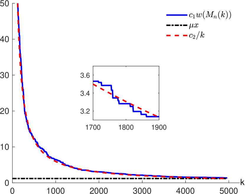
Our preliminary conjecture on how the sum of these weights will change in the uniformly weighted setup is given in Figure 4. In this figure, we consider two scenarios: i.) and and ii.) and In both the scenarios, the weights of the -faces are i.i.d. uniform random variables which are revealed one at a time in an arbitrary order. That is, the weight of each -face is initially presumed to be which then gets replaced with the actual value when it gets revealed. Accordingly, we begin with an arbitrary -MSA and then sequentially update it as the weight of a new face gets revealed.
Let denote the updated -MSA after the weight of the -th face is revealed. Also, let and for The blue and red curves in the figure show the value of and respectively. The red curve is our guess for based on the results in this paper. Finally, the black curve shows the constant value Clearly, the blue and red curves closely match and they both get close to the black one as the value of increases.

Some of the other directions that we wish to pursue in the future are as follows.
-
1.
Geometric random graphs and complexes: Extending our results from the Erdős-Rényi and Linial-Meshulam models to geometric random graphs and geometric complexes and understanding differences between the two scenarios.
-
2.
Large deviation results and central limit theorems: Obtaining general large deviation results for the Kolmogorov distance between and as well as central limit theorems characterizing the variance of the weight distribution.
-
3.
Rates of convergence: Deriving the rate at which converges to
Acknowledgments
The authors would like to thank Matthew Kahle, Omer Bobrowski, Primoz Skraba, Ron Rosenthal, Robert Adler, Christina Goldschmidt, D. Yogeshwaran, and Takashi Owada for useful suggestions. A portion of this work was done when Gugan Thoppe was a postdoc with Sayan Mukherjee at Duke University.
References
- [1] Robert Adler. TOPOS: Pinsky was wrong, Euler was right. \urlhttps://imstat.org/2014/11/18/topos-pinsky-was-wrong-euler-was-right/, 2014. [Online; accessed 14-Nov.-2020].
- [2] Paul Erdős and Alfred Rényi. On random graphs I. Publicationes Mathematicae Debrecen, 6(290-297):18, 1959.
- [3] Paul Erdős and Alfred Rényi. On the evolution of random graphs. Publ. Math. Inst. Hungary. Acad. Sci., 5:17–61, 1960.
- [4] Alan M Frieze. On the value of a random minimum spanning tree problem. Discrete Applied Mathematics, 10(1):47–56, 1985.
- [5] Masanori Hino and Shu Kanazawa. Asymptotic behavior of lifetime sums for random simplicial complex processes. Journal of the Mathematical Society of Japan, 2019.
- [6] Matthew Kahle and Boris Pittel. Inside the critical window for cohomology of random k-complexes. Random Structures & Algorithms, 48(1):102–124, 2016.
- [7] Gil Kalai. Enumeration of Q-acyclic simplicial complexes. Israel Journal of Mathematics, 45(4):337–351, 1983.
- [8] Nathan Linial and Roy Meshulam. Homological connectivity of random 2-complexes. Combinatorica, 26(4):475–487, 2006.
- [9] Nathan Linial, Ilan Newman, Yuval Peled, and Yuri Rabinovich. Extremal problems on shadows and hypercuts in simplicial complexes. arXiv preprint arXiv:1408.0602, 2014.
- [10] Nathan Linial and Yuval Peled. On the phase transition in random simplicial complexes. Annals of Mathematics, pages 745–773, 2016.
- [11] Roy Meshulam and Nathan Wallach. Homological connectivity of random k-dimensional complexes. Random Structures & Algorithms, 34(3):408–417, 2009.
- [12] Primoz Skraba, Gugan Thoppe, and D Yogeshwaran. Randomly Weighted - complexes: Minimal Spanning Acycles and Persistence Diagrams. Electronic Journal of Combinatorics, 27(2), 2019.
- [13] Matthew Kahle. Topology of random simplicial complexes: a survey. AMS Contemporary Mathematics, 620, 201–222, 2014.
[nico]
Nicolas Fraiman
Assistant Professor
University of North Carolina at Chapel Hill
Chapel Hill, NC, United States
fraiman\imageatemail\imagedotunc\imagedotedu
\urlhttps://fraiman.web.unc.edu/
{authorinfo}[sayan]
Sayan Mukherjee
Professor
Duke University,
Durham, NC, United States
Center for Scalable Data Analytics and Artificial Intelligence, Universität Leipzig
Max Planck Institute for Mathematics in the Sciences
Leipzig, Saxony, Germany
sayan.mukherjee\imageatmis\imagedotmpg\imagedotde
\urlhttps://sayanmuk.github.io/
{authorinfo}[gugan]
Gugan Thoppe
Assistant Professor
Indian Institute of Science
Bengaluru, India
gthoppe\imageatiisc\imagedotac\imagedotin
\urlhttps://sites.google.com/site/gugancth/