The role of local bounds on neighborhoods in the network for scale-free state synchronization of multi-agent systems

Anton A. Stoorvogel, Ali Saberi, and Zhenwei Liu Anton A. Stoorvogel is with Department of Electrical Engineering, Mathematics and Computer Science, University of Twente, P.O. Box 217, Enschede, The Netherlands (e-mail: [email protected])Ali Saberi is with School of Electrical Engineering and Computer Science, Washington State University, Pullman, WA 99164, USA (e-mail: [email protected])Zhenwei Liu is with College of Information Science and Engineering, Northeastern University, Shenyang 110819, China (e-mail: [email protected])

Abstract

This paper provides necessary and sufficient conditions for the existence of solutions to the state synchronization problem of homogeneous multi-agent systems (MAS) via scale-free linear dynamic non-collaborative protocol in both continuous and discrete time. These conditions guarantee for which class of MAS, one can achieve scale-free state synchronization. We investigate protocol design with and without utilizing local bounds on the neighborhood of agents. The results shows that the availability of local bounds on neighborhoods plays a key role.

1 Introduction

The synchronization problem for multi-agent systems (MAS) has attracted substantial attention due to the wide potential for applications in several areas, such as autonomous vehicles, satellites/robots system, distributed sensor network, and smart gird (power grid), see for instance the books [1, 2, 4, 11, 15, 16, 22] and references [7, 13, 14].

Traditionally, we used networks described by Laplacian matrices for continuous-time systems. In early work for discrete-time systems, such as [12, 21, 5, 6], the networks were described by row-stochastic matrices. In the literature, it was never really clarified why one would use Laplacian matrices in continuous-time and row-stochastic matrices in discrete-time. In this early work, researchers generally assumed the network was known. In that case, the distinction between Laplacian and row-stochastic matrices is not that crucial because we can easily convert one in the other if some bounds are known for the network as outlined below.

Later, the proposed protocols in the literature for synchronization of MAS still assumed some knowledge of the communication network such as bounds on the spectrum of the associated Laplacian matrix and the number of agents. In this context, knowing an upper bound for the Laplacian was viewed as reasonable and the distinction between Laplacian and row-stochastic matrices was therefore not viewed as crucial.

As it is pointed out in [17, 18, 19, 20], the protocols traditionally designed for synchronization suffer from scale fragility. In particular, they showed that almost all existing protocol designs at that time failed to achieve synchronization when the network becomes too large (unless the protocol is adapted based on the size of the network).

In the past few years, scale-free linear protocol design has been subject of research in MAS literature to deal with the existing scale fragility in MAS [8]. In a “scale-free” design the proposed protocols are designed solely based on the knowledge of agent models and do not depend on

•

Information about the communication network such as the spectrum of the associated Laplacian matrix.
•

Knowledge about the number of agents.

In the context of scale-free protocol design, the distinction between networks described by Laplacian matrices and row-stochastic matrices is actually crucial. One can only convert Laplacian matrices to row-stochastic matrices if you have some information about the network. To be more precise, each agent should have a local bound on the weighted in-degree of the network.

This brings us to a crucial question. If this local bound is not available for discrete-time systems (and we cannot convert the Laplacian matrix to a row-stochastic matrix), can we then still obtain a linear scale-free protocol? It is also interesting to investigate whether this local bound can help us in continuous-time systems.

The results in this paper are as follows, which are essentially necessary conditions for scale-free synchronization of linear MAS:

•

For discrete-time systems without availability of local bounds it is impossible to obtain scale-free synchronization.
•

For discrete-time systems using local bounds it is possible to obtain scale-free synchronization provided the agents are neutrally stable.
•

For continuous-time systems without availability of local bounds we effectively need that agents are neutrally stable, minimum-phase and of relative degree $1$ .
•

For continuous-time systems using local bounds we only need that agents are neutrally stable.

The surprising result of this paper is that in discrete-time without local bounds we can no longer achieve scale-free synchronization. For continuous-time agents it is still possible without local bounds to achieve scale-free synchronization but we need additional restrictions on the agents namely minimum-phase and relative degree $1$ .

Notation and background

Given a matrix $A\in\mathbb{R}^{m\times n}$ , $A^{\mbox{\tiny T}}$ and $A^{*}$ denote its transpose and conjugate transpose respectively. $I$ denotes the identity matrix and $0$ denotes the zero matrix where the dimension is clear from the context.

To describe the information flow among the agents we associate a weighted graph $\mathcal{G}$ to the communication network. The weighted graph $\mathcal{G}$ is defined by a triple $(\mathcal{V},\mathcal{E},\mathcal{A})$ where $\mathcal{V}=\{1,\ldots,N\}$ is a node set, $\mathcal{E}$ is a set of pairs of nodes indicating connections among nodes, and $\mathcal{A}=[a_{ij}]\in\mathbb{R}^{N\times N}$ is the weighted adjacency matrix with non negative elements $a_{ij}$ . Each pair in $\mathcal{E}$ is called an edge, where $a_{ij}>0$ denotes an edge $(j,i)\in\mathcal{E}$ from node $j$ to node $i$ with weight $a_{ij}$ . Moreover, $a_{ij}=0$ if there is no edge from node $j$ to node $i$ . We assume there are no self-loops, i.e. we have $a_{ii}=0$ . A path from node $i_{1}$ to $i_{k}$ is a sequence of nodes $\{i_{1},\ldots,i_{k}\}$ such that $(i_{j},i_{j+1})\in\mathcal{E}$ for $j=1,\ldots,k-1$ . A directed tree is a subgraph (subset of nodes and edges) in which every node has exactly one parent node except for one node, called the root, which has no parent node. A directed spanning tree is a subgraph which is a directed tree containing all the nodes of the original graph. If a directed spanning tree exists, the root has a directed path to every other node in the tree [3].

For a weighted graph $\mathcal{G}$ , the matrix $L=[\ell_{ij}]$ with

\ell_{ij}=\left\{\;\begin{array}[]{cl}\sum_{k=1}^{N}a_{ik},&i=j,\\ -a_{ij},&i\neq j,\end{array}\right.

is called the Laplacian matrix associated with the graph $\mathcal{G}$ . The Laplacian matrix $L$ has all its eigenvalues in the closed right half plane and at least one eigenvalue at zero associated with right eigenvector 1 [3]. Moreover, if the graph contains a directed spanning tree, the Laplacian matrix $L$ has a single eigenvalue at the origin and all other eigenvalues are located in the open right-half complex plane [15].

The invariant zeros of a linear system with realization $(A,B,C,D)$ are defined as all $s\in\mathbb{C}$ for which

\begin{pmatrix}sI-A&-B\\ C&D\end{pmatrix}

(1)

loses rank. For a linear system with transfer matrix $G$ which is single input and/or single output then the invariant zeros can be easily defined as those $s\in\mathbb{C}$ for which $G(s)=0$ .

The system is called minimum phase if all invariant zeros are in the open left half plane (continuous-time) or in the open unit disc (discrete-time). The system is called weakly minimum-phase if all invariant zeros are in the closed left half plane (continuous-time) or in the closed unit disc (discrete-time) while the invariant zeros on the boundary are semi-simple. For a linear system with transfer matrix $G$ which is single input (SIMO) and/or single output (MISO), an invariant zero $s_{0}$ is semi-simple if and only if

\lim_{s\rightarrow s_{0}}\frac{1}{s-s_{0}}G(s)

is well-defined and unequal to zero.

A single-input/single-output (SISO) linear system $(A,B,C)$ , has relative degree 1 if $CB\neq 0$ . The system has relative degree $r>1$ , whenever $CA^{r-1}B\neq 0$ while $CA^{r-2}B=0$ . A multi-input/multi-output (MIMO) linear system $(A,B,C)$ , has has uniform rank with order of infinite zeros equal to one if

\operatorname{rank}\begin{pmatrix}sI-A&-B\\ C&D\end{pmatrix}=\operatorname{rank}CB

for almost all $s\in\mathbb{C}$ .

2 Multi-agent systems and local bounds on neighborhoods in the network

Consider a multi-agent systems (MAS) consisting of $N$ identical agents:

\begin{array}[]{ccl}x_{i}^{+}(t)&=&Ax_{i}(t)+Bu_{i}(t),\\ y_{i}(t)&=&Cx_{i}(t),\end{array}

(2)

where $x_{i}(t)\in\mathbb{R}^{n}$ , $y_{i}(t)\in\mathbb{R}^{p}$ and $u_{i}(t)\in\mathbb{R}^{m}$ are the state, output, and input of agent $i$ , respectively, with $i=1,\ldots,N$ . In the aforementioned presentation, for continuous-time systems, $x_{i}^{+}(t)=\dot{x}_{i}(t)$ with $t\in\mathbb{R}$ while for discrete-time systems, $x_{i}^{+}(t)=x_{i}(t+1)$ with $t\in\mathbb{Z}$ .

The communication network provides each agent with a linear combination of its own output relative to that of other neighboring agents. In particular, each agent $i\in\{1,\cdots,N\}$ has access to the quantity:

\zeta_{i}(t)=\sum_{j=1,j\neq i}^{N}a_{ij}(y_{i}(t)-y_{j}(t)).

(3)

where $a_{ij}\geqslant 0$ , $a_{ii}=0$ for $i,j\in\{1,\ldots,N\}$ . The topology of the network can be described by a graph $\mathcal{G}$ with nodes corresponding to the agents in the network and edges given by the nonzero coefficients $a_{ij}$ . In particular, $a_{ij}>0$ implies that an edge exists from agent $j$ to $i$ . The weight of the edge equals the magnitude of $a_{ij}$ .

We can express the communication in the network in terms of the Laplacian matrix $L$ associated with this weighted graph $\mathcal{G}$ . In particular, $\zeta_{i}$ can be rewritten as:

\zeta_{i}(t)=\sum_{j=1}^{N}\ell_{ij}y_{j}(t).

(4)

where $L=[\ell_{ij}]$ is the Laplacian matrix associated with the communication network with

\ell_{ij}=-a_{ij}\;\;(i\neq j),\qquad\ell_{ii}=\sum_{j=1}^{N}a_{ij}

for $i,j=1,\ldots,N$ where $a_{ij}$ is the weight of the edge from node $j$ to node $i$ if such an edge exists and $a_{ij}=0$ if such an edge does not exist.

Note that $\ell_{ii}$ can be referred to as the local weighted in-degree of the graph, often denoted in the literature as $d_{\text{in}}(i)$ , since we have:

\ell_{ii}=d_{\text{in}}(i):=\sum_{j=1}^{N}a_{ij}

For the design of protocols it has turned out to be useful to have a bound for the local weighted in-degree of the graph. The paper [20] considers globally bounded neighborhoods in the sense that there exists a global bound $q$ for the in-degree:

d_{\text{in}}(i)<q

for all agents $i=1,\ldots,N$ .

In scale-free protocols, we are looking for protocols which do not depend on the network structure. This is motivated by the fact that in many applications, an agent might be added/removed or a link might fail and you then do not want to have to redesign the protocols being used. This makes using such a global bound undesirable.

However, in most cases it turns out that it is sufficient if agent $i$ has a local bound available to $d_{in}(i)$ . Note that this is actually a reasonable assumption because it is really a local bound since it only bounds the weight of the edges going into node $i$ and does not rely on the rest of the network.

We refer to the property where agent $i$ has a bound $q_{i}$ available with

q_{i}>d_{\text{in}}(i)

(5)

for $i=1,\ldots,N$ as locally bounded neighborhoods. In that case, we can define

\tilde{\zeta}_{i}(t)=\frac{1}{1+q_{i}}\zeta_{i}(t)

and we obtain:

\tilde{\zeta}_{i}(t)=\sum_{j=1,j\neq i}^{N}d_{ij}(y_{i}(t)-y_{j}(t)),

(6)

where

d_{ij}=\frac{a_{ij}}{1+q_{i}},

for $i\neq j$ while

d_{ii}=1-\sum_{j=1,j\neq i}^{N}d_{ij}

Note that the weight matrix $D=[d_{ij}]$ is then a, so-called, row stochastic matrix. If we design a protocol based on these scaled data:

\left\{\;\begin{array}[]{cl}x_{i,c}^{+}&=A_{c}x_{i,c}+B_{c}\tilde{\zeta}_{i},\\ u_{i}&=F_{c}x_{i,c},\end{array}\right.

(7)

where $A_{c}$ , $B_{c}$ and $F_{c}$ are independent of the network structure then we implement this protocol for the original network as:

\left\{\;\begin{array}[]{cl}x_{i,c}^{+}&=A_{c}x_{i,c}+\frac{1}{1+q_{i}}B_{c}\zeta_{i},\\ u_{i}&=F_{c}x_{i,c},\end{array}\right.

(8)

where $x_{c,i}(t)\in\mathbb{R}^{n_{c}}$ is the state of protocol.

Traditionally, in continuous-time multi-agent systems we have used the Laplacian matrix and we have not used these local bounds. On the other hand for discrete-time multi-agent systems in the literature we have always used the row stochastic matrix and we therefore implicitly assumed knowledge of these local bounds on the network.

This paper will investigate, for both continuous-time and discrete-time multi-agent systems, whether the use of these local bounds can improve design possibilities for scale-free protocols that achieve synchronization.

We first need a definition before we give a precise problem formulation.

Definition 1

We define the set $\mathbb{G}^{N}$ as the set of all directed graphs of $N$ agents which contain a directed spanning tree.

We formulate the scale-free or scale-free synchronization problem of a MAS as follows.

Problem 1

The scale-free state synchronization problem without local bounds for MAS (2) with communication given by (4) is to find, if possible, a fixed linear protocol of the form:

\left\{\;\begin{array}[]{cl}x_{i,c}^{+}&=A_{c}x_{i,c}+B_{c}\zeta_{i},\\ u_{i}&=F_{c}x_{i,c},\end{array}\right.

(9)

where $x_{c,i}(t)\in\mathbb{R}^{n_{c}}$ is the state of protocol, such that state synchronization is achieved, i.e.

\lim_{t\rightarrow\infty}x_{i}(t)-x_{j}(t)=0

(10)

for all $i,j=1,\ldots,N$ for any number of agents $N$ , for any fixed communication graph $\mathcal{G}\in\mathbb{G}^{N}$ and for all initial conditions of agents and protocols.

Problem 2

The scale-free state synchronization problem with local bounds for MAS (2) with communication given by (4) is to find, if possible, a fixed linear protocol of the form (8) , such that state synchronization (10) is achieved for any number of agents $N$ , any $q_{1},\ldots q_{N}\in\mathbb{R}^{+}$ , for any fixed communication graph $\mathcal{G}\in\mathbb{G}^{N}$ satisfying (5) and for all initial conditions of agents and protocols.

In both problems the protocol parameters $A_{c}$ , $B_{c}$ and $F_{c}$ are designed completely independent of the network structure. They only rely on the agent model, i.e. $A$ , $B$ and $C$ . The only but intrinsic difference between these two problems is that in Problem 2 we added an initial scaling of the measurements based on a local bound for the weighted in-degree.

Effectively, in Problem 1 we use communication described by a Laplacian matrix while in Problem 2 by using (6) we use communication described by a row-stochastic matrix which requires the availability of these local bounds. Classically, Problem 1 would be standard for continuous-time systems and Problem 2 would be standard for discrete-time systems. We should note that in many papers discrete-time problems are immediately defined in terms of the row-stochastic matrix without making the scaling explicit.

3 Continuous-time results

As indicated before we are going to investigate solvability of problems 1 and 2 for continuous-time systems. We will in the next subsection consider Problem 1 where we use the classical Laplacian matrix and then we will consider in the subsection thereafter Problem 2 where we used the local bounds to convert the Laplacian matrix into a row-stochastic matrix.

3.1 Scale-free synchronization without locally bounded neighborhoods

In this section, we consider scale-free synchronization for continuous-time systems with a network described by a Laplacian matrix. We want to find conditions whether Problem 1 is solvable for this class of systems. In other words, we have no information available about the network and want to design a protocol that achieves synchronization. We first establish necessary conditions and then sufficient conditions.

3.1.1 Necessary conditions

Theorem 1

Consider the scale-free state synchronization problem without local bounds as formulated in Problem 1 for continuous-time systems.

Part 1:

The scale-free state synchronization problem without local bounds is solvable with a scalar input and/or a scalar output only if the agent model (2) is either asymptotically stable or satisfies the following conditions:

1.

Stabilizable and detectable,
2.

Neutrally stable,
3.

Weakly minimum phase,
4.

Relative degree equal to 1.

Part 2:

The scale-free state synchronization problem without local bounds is solvable for multi-input/multi-output agents only if the agent model (2) is:

1.

Stabilizable and detectable,
2.

All poles are in the closed left half plane.

Remark 1

The paper [19, Theorem 4.1] shows that there is no linear static protocol which can achieve scale-free synchronization for MAS modeled as a chain of $n$ integrators ( $n\geqslant 2$ ) with full state coupling. Theorem 1 in this paper extends the result of [19]. We prove that there is no linear dynamic protocol either to achieve scale-free synchronization for this class of MAS.

Remark 2

In [9], we provided necessary conditions for MAS consisting of SISO agent. Here we have obtained the necessary conditions for MAS consisting of SIMO, MISO, or MIMO agents.

Remark 3

We would like to point out that the conditions of neutral stability and weakly minimum phase, which are necessary in the SISO case, are not necessary in the MIMO case as illustrated in following examples.

Example 1

To illustrate that neutrally stable is not a necessary condition for MIMO systems consider the system (2) with:

A=\begin{pmatrix}0&1\\ 0&0\end{pmatrix},\quad B=\begin{pmatrix}1&0\\ 0&1\end{pmatrix},\quad C=\begin{pmatrix}1&0\\ 0&1\end{pmatrix}.

Clearly, the system is not neutrally stable but it is easy to verify that the protocol $u_{i}=-\zeta_{i}$ will achieve scale-free state synchronization.

Example 2

To illustrate that in the MIMO case in some peculiar cases the system can even have zeros in the open right half plane while scale-free state synchronization problem is still possible, consider the system (2) with:

A=\begin{pmatrix}0&0&1\\ 0&-1&1\\ 0&0&-1\end{pmatrix},\quad B=\begin{pmatrix}1&0\\ 0&0\\ 0&1\end{pmatrix},\quad C=\begin{pmatrix}1&0&0\\ 0&1&-2\end{pmatrix}.

It is easily verified that the system has an invariant zero in $1$ but the protocol

u_{i}=\begin{pmatrix}-1&0\\ 0&0\end{pmatrix}\zeta_{i}

will achieve scale-free state synchronization. Effectively, we see that we can have non-minimum phase agents, if the agent with transfer matrix $G$ can be stabilized by a controller with transfer matrix $G_{c}$ such that $GG_{c}$ has no unstable zeros. In other words, the unstable zero can be canceled without an unstable pole-zero cancellation. This only happens in cases such as the above example where one channel contains stable, non-minimum phase dynamics and another channel contains unstable, minimum phase dynamics. Clearly this cannot be done in a MISO, SIMO or SISO system where we effectively have only one channel available for feedback.

Proof of Theorem 1: The necessity of stabilizability and detectability is obvious. By using protocol (9) and defining

\tilde{A}=\begin{pmatrix}A&BF_{c}\\ 0&A_{c}\end{pmatrix},\qquad\tilde{B}=\begin{pmatrix}0\\ B_{c}\end{pmatrix},\qquad\tilde{C}=\begin{pmatrix}C&0\end{pmatrix}

(11)

then [16, Chapter 3] has shown that we achieve synchronization if

\tilde{A}+\lambda_{i}\tilde{B}\tilde{C}

is Hurwitz stable for all nonzero eigenvalues $\{\lambda_{2},\ldots,\lambda_{N}\}$ of the Laplacian matrix $L$ . Since, we are looking for a scale-free protocol which works for any network in $\mathbb{G}^{N}$ . we need that

\tilde{A}+\lambda\tilde{B}\tilde{C}

(12)

is Hurwitz stable for all $\lambda\in\mathbb{C}$ with $\operatorname{Re}\lambda>0$ .

The SISO result has been presented before in [9, Theorem 1]. In the multi-input and single-output case, we can follow the arguments provided in the proof of that paper to conclude that, for an agent with transfer matrix $G$ /and a protocol with transfer agent $G_{c}$ , we need that $GG_{c}$ (which is a scalar rational function) is positive-real and hence needs to be neutrally stable, weakly minimum-phase and relative degree $1$ .

Clearly the Hurwitz stability of (12) requires the transfer matrix of the system:

\dot{p}=(\tilde{A}+\lambda\tilde{B}\tilde{C})p+\begin{pmatrix}B\\ 0\end{pmatrix}v,\qquad\quad z=\tilde{C}p

to be asymptotically stable which implies:

(I-\lambda GG_{c})^{-1}G

(13)

is asymptotically stable. If $G$ has a repeated pole on the imaginary axis then this can only be cancelled by the scalar transfer function $(I-\lambda GGc)^{-1}$ if $GG_{c}$ has a repeated pole on the imaginary axis which leads to a contradiction since $GG_{c}$ was neutrally stable.

Similarly the Hurwitz stability of (12) requires the transfer matrix of the system:

\dot{p}=(\tilde{A}+\lambda\tilde{B}\tilde{C})p+\tilde{B}v,\qquad\quad z=\begin{pmatrix}0&F_{c}\end{pmatrix}p

to be asymptotically stable which implies:

G_{c}(I-\lambda GG_{c})^{-1}

(14)

is asymptotically stable and strictly proper.

If $G$ has a repeated invariant zero $s_{0}$ on the imaginary axis then for $GG_{c}$ to be weakly minimum-phase we need that $G_{c}$ has a pole in $s_{0}$ . It can be easily verified that this yields a contradiction with (14) being asymptotically stable.

Finally, if $G$ has relative degree $2$ or higher, then $GG_{c}$ can never have relative degree $1$ for a strictly proper protocol of the form 9.

The above argument can be easily modified for the single-input and multi-output case, where we again follow the arguments provided in the proof of [9, Theorem 1] to conclude this time that $G_{c}G$ (instead of $GG_{c}$ ) is positive-real and hence needs to be neutrally stable, weakly minimum-phase and relative degree $1$ . Since, in this case, $G_{c}G$ is a scalar transfer function the rest of the above arguments can be easily modified.

For MIMO systems, we also need that (12) is Hurwitz stable for all $\lambda\in\mathbb{C}$ with $\operatorname{Re}\lambda>0$ . Since $\lambda$ can be arbitrarily small it is obvious that (12) Hurwitz stable for all $\lambda\in\mathbb{C}$ with $\operatorname{Re}\lambda>0$ requires that the eigenvalues of $\tilde{A}$ have to be in the closed left half plane which trivially implies that the eigenvalues of $A$ have to be in the closed left half plane

3.1.2 Sufficient conditions

Theorem 2

The scale-free state synchronization problem without local bounds as formulated in Problem 1 is solvable if the continuous-time agent model (2) is either asymptotically stable or satisfies the following conditions:

1.

Stabilizable and detectable,
2.

Neutrally stable,
3.

Minimum phase,
4.

Agent model has uniform rank with order of infinite zero equal to one.

Remark 4

Note that the sufficient conditions of Theorem 2 are very close to the necessary conditions of Theorem 1 for single-input or single-output systems. We only strengthen the requirement of weakly minimum phase to minimum phase.

For MIMO systems the gap between necessary and sufficient conditions is much larger but only because of some very peculiar cases like the ones in Example 1 and 2. We claim that generically the necessary conditions for the SISO case also apply in the MIMO case.

Proof: This result has been presented before in [9, Theorem 3].

Note that in [9] we have also presented simulations to see how these protocols perform.

3.2 Scale-free synchronization with locally bounded neighborhoods

3.2.1 Necessary conditions

Theorem 3

Consider the scale-free state synchronization problem with local bounds as formulated in Problem 2 for continuous-time agents.

Part 1:

The scale-free state synchronization problem with local bounds is solvable with a scalar input and/or a scalar output only if the agent model (2) is either asymptotically stable or satisfies the following conditions:

1.

Stabilizable and detectable,
2.

Neutrally stable.

Part 2:

The scale-free state synchronization problem with local bounds is solvable for MIMO agents only if the agent model (2) is:

1.

Stabilizable and detectable,
2.

All poles are in the closed left half plane.

Remark 5

For agents with a scalar input and/or a scalar output the conditions are actually necessary and sufficient as we will see in the next subsection.

Proof: The necessity of stabilizability and detectability is obvious. By using protocol (7) and defining (11) then [16, Chapter 3] has shown that we achieve synchronization if

\tilde{A}+(1-\lambda_{i})\tilde{B}\tilde{C}

(15)

is Hurwitz stable for all eigenvalues $\{\lambda_{2},\ldots,\lambda_{N}\}$ of the row stochastic matrix $D$ unequal to $1$ . For a network in $\mathbb{G}^{N}$ , we find that $|\lambda_{i}|<1$ for $i=2,\ldots,N$ . Moreover, it is clear that for any $\lambda$ with $|\lambda|<1$ , there exists a network in $\mathbb{G}^{N}$ whose associated row stochastic matrix has an eigenvalue in $\lambda$ .

Since, we are looking for a scale-free protocol which works for any network in $\mathbb{G}^{N}$ . we need that

\tilde{A}+(1-\lambda)\tilde{B}\tilde{C}

(16)

is Hurwitz stable for all $\lambda$ with $|\lambda|<1$ .

Using arguments similar to [9, Theorem 2] we note that we need that $GG_{c}+\tfrac{1}{2}$ is positive real (single-output case) or $G_{c}G+\tfrac{1}{2}$ is positive real (single-input case). We can then use similar arguments as in the proof of Theorem 1 to conclude that $G$ needs to be neutrally stable.

For the general MIMO case we note that in (16), the $\lambda$ can be arbitrarily close to $1$ , and therefore the eigenvalues of $\tilde{A}$ have to be in the closed left half plane which trivially implies that the eigenvalues of $A$ have to be in the closed left half plane

3.2.2 Sufficient conditions

Theorem 4

The scale-free state synchronization problem with local bounds as formulated in Problem 2 is solvable if the continuous-time agent model (2) is either asymptotically stable or satisfies the following conditions:

1.

Stabilizable and detectable,
2.

Neutrally stable.

Remark 6

We see that the availability of these local bounds and being able to convert the Laplacian matrix into a row-stochastic matrix allows us to solve our problem without imposing any constraints on the invariant zeros of the system or the relative degree.

The only gap between our necessary and sufficient conditions is for MIMO systems where necessity only requires the poles to be in the closed left half plane while our sufficient conditions impose neutral stability. That neutral stability is not necessary in this case is illustrated by the system in Example 1.

Proof: We first note that since the system is neutrally stable there exists $P>0$ such that

A^{\mbox{\tiny T}}P+PA\leqslant 0.

Next, we consider the protocol

\begin{array}[]{ccl}\dot{\chi}_{i}&=&(A+HC)\chi_{i}-H\tilde{\zeta}_{i}\\ u_{i}&=&-\delta B^{\mbox{\tiny T}}P\chi_{i}\end{array}

(17)

where $H$ is such that $A+HC$ is Hurwitz stable and $\delta>0$ needs to be small enough as will become clear later.

Since $A+HC$ is Hurwitz stable there exists $\varepsilon>0$ and $Q>0$ such that

(A+HC)^{\mbox{\tiny T}}Q+Q(A+HC)+\varepsilon Q+I=0

(18)

Next we choose $\delta>0$ such that:

2\delta(QBB^{\mbox{\tiny T}}P+PBB^{\mbox{\tiny T}}Q)\leqslant\varepsilon Q

(19)

By using protocol (17) and defining

\tilde{A}=\begin{pmatrix}A&-\delta BB^{\mbox{\tiny T}}P\\ 0&A+HC\end{pmatrix},\qquad\tilde{B}=\begin{pmatrix}0\\ -H\end{pmatrix},\qquad\tilde{C}=\begin{pmatrix}C&0\end{pmatrix}

(20)

then (as argued in the proof of Theorem 3), we need that

\tilde{A}+(1-\lambda)\tilde{B}\tilde{C}

(21)

is Hurwitz stable for all $\lambda$ with $|\lambda|<1$ .

We need to prove that the interconnection of (17) and (2) with $\tilde{\zeta}_{i}=(1-\lambda)y_{i}$ is asymptotically stable for all $\lambda$ with $|\lambda|<1$ . The dynamics associated with the matrix (21) are given by:

\begin{array}[]{ccl}\dot{\varphi}&=&A\varphi-\delta BB^{\mbox{\tiny T}}P\psi\\ \dot{\psi}&=&(A+HC)\psi-(1-\lambda)HC\varphi\end{array}

Choosing

\tilde{\varphi}=(1-\lambda)\varphi\quad\text{ and }\quad e=\psi-\tilde{\varphi}

we obtain:

\begin{array}[]{ccl}\dot{\tilde{\varphi}}&=&A\tilde{\varphi}-\delta(1-\lambda)BB^{\mbox{\tiny T}}P(e+\tilde{\varphi})\\ \dot{e}&=&(A+HC)e+\delta(1-\lambda)BB^{\mbox{\tiny T}}P(e+\tilde{\varphi})\end{array}

We note that (18) and (19) imply that:

[A+HC+\delta(1-\lambda)BB^{\mbox{\tiny T}}P]^{*}Q+Q[A+HC+\delta(1-\lambda)BB^{\mbox{\tiny T}}P]+I\leqslant 0

Define $V_{1}=e^{*}Qe$ and we obtain:

	$\displaystyle\dot{V}_{1}$	$\displaystyle\leqslant-e^{}e+\delta(1-\lambda)e^{}QBB^{\mbox{\tiny T}}P\tilde{\varphi}+\delta(1-\lambda^{})\tilde{\varphi}^{}PBB^{\mbox{\tiny T}}Qe$
		$\displaystyle\leqslant-e^{}e+4\delta e^{}QBB^{\mbox{\tiny T}}Qe+\tfrac{1}{4}\delta\|1-\lambda\|^{2}\tilde{\varphi}^{*}PBB^{\mbox{\tiny T}}P\tilde{\varphi}$

Next, we consider $V_{2}=\tilde{\varphi}^{*}P\tilde{\varphi}$ and we obtain:

	$\displaystyle\dot{V}_{2}$	$\displaystyle=\tilde{\varphi}^{}(A^{\mbox{\tiny T}}P+PA)\tilde{\varphi}-\delta(1-\lambda)\tilde{\varphi}^{}PBB^{\mbox{\tiny T}}P(e+\tilde{\varphi})-\delta(1-\lambda^{})(e+\tilde{\varphi})^{}PBB^{\mbox{\tiny T}}P\tilde{\varphi}$
		$\displaystyle\leqslant-\delta\|1-\lambda\|^{2}\tilde{\varphi}^{}PBB^{\mbox{\tiny T}}P\tilde{\varphi}-\delta(1-\lambda)\delta\tilde{\varphi}^{}PBB^{\mbox{\tiny T}}Pe-\delta(1-\lambda^{})e^{}PBB^{\mbox{\tiny T}}P\tilde{\varphi}$
		$\displaystyle\leqslant-\tfrac{3}{4}\delta\|1-\lambda\|^{2}\tilde{\varphi}^{}PBB^{\mbox{\tiny T}}P\tilde{\varphi}+4\delta e^{}PBB^{\mbox{\tiny T}}Pe$

where we used that $|\lambda|<1$ implies

|1-\lambda|^{2}\leqslant 2\operatorname{Re}(1-\lambda).

(22)

Combining the above inequalities and choose $\delta$ small enough such that $8\delta(PBB^{\mbox{\tiny T}}P+QBB^{\mbox{\tiny T}}Q)<I$ , we find:

\dot{V}_{1}+\dot{V}_{2}\leqslant-\tfrac{1}{2}e^{*}e-\tfrac{1}{2}\delta|1-\lambda|^{2}\tilde{\varphi}^{*}PBB^{\mbox{\tiny T}}P\tilde{\varphi}

from which asymptotically stability follows using a standard argument based on LaSalle invariance principle.

4 Discrete–time results

Next, we are going to investigate solvability of problems 1 and 2 for discrete-time systems. We will in the next subsection consider Problem 1 where we use the Laplacian matrix and then we will consider in the subsection thereafter Problem 2 where we used the local bounds to convert the Laplacian matrix into a row-stochastic matrix. The latter is the classical case for discrete-time systems.

4.1 Scale-free synchronization without locally bounded neighborhoods

Theorem 5

The scale-free state synchronization problem without local bounds as formulated in Problem 1 is NOT solvable except for the trivial case when the agents are asymptotically stable.

Proof: Consider a protocol (9). Then similarly as in the proof of Theorem 1, we can define (11) and argue that

\tilde{A}+\lambda\tilde{B}\tilde{C}

must be Schur stable (eigenvalues in open unit disc) for all $\lambda\in\mathbb{C}$ with $\operatorname{Re}\lambda>0$ . Assume this is true. Consider:

\det(sI-\tilde{A}-\lambda\tilde{B}\tilde{C})

(23)

If this determinant does not depend on $\lambda$ then

\det(sI-\tilde{A}+\lambda\tilde{B}\tilde{C})=\det(sI-\tilde{A})

and if this is asymptotically stable then $\tilde{A}$ must be Schur stable which is only possible if the matrix $A$ is already Schur stable. Note that the coefficients of a characteristic polynomial of a Schur stable matrix of fixed dimensions can never exceed a certain bound $M$ since all eigenvalues are bounded. But if (23) depends on $\lambda$ then for large enough $\lambda$ the coefficients of this characteristic polynomial will exceed this bound $M$ which implies that the matrix is not Schur stable which yields a contradiction.

4.2 Scale-free synchronization with locally bounded neighborhoods

4.2.1 Necessary conditions

Theorem 6

Consider the scale-free state synchronization problem with local bounds as formulated in Problem 2 for discrete-time systems.

Part 1:

The scale-free state synchronization problem with local bounds is solvable for single-input or single-output agents only if the agent model (2) is either asymptotically stable or satisfies the following conditions:

1.

Stabilizable and detectable,
2.

Neutrally stable.

Part 2:

The scale-free state synchronization problem with local bounds is solvable for MIMO agents only if the agent model (2) is:

1.

Stabilizable and detectable,
2.

All poles are in the closed unit disc.

Remark 7

In the single-input or single-output case the conditions are actually necessary and sufficient as we will see in the next subsection.

Proof: The arguments are identical to the proof of the continuous-time result in Theorem 3. In other words, we achieve synchronization if

\tilde{A}+(1-\lambda_{i})\tilde{B}\tilde{C}

is Schur stable for all eigenvalues $\{\lambda_{2},\ldots,\lambda_{N}\}$ unequal to $1$ of the row stochastic matrix $D$ .

For the general MIMO case we note that the $\lambda$ can be arbitrarily close to $1$ , and therefore the eigenvalues of $\tilde{A}$ have to be in the closed unit disc which trivially implies that the eigenvalues of $A$ have to be in the closed unit disc.

4.2.2 Sufficient conditions

Theorem 7

The scale-free state synchronization problem with local bounds as formulated in Problem 2 is solvable if the discrete-time agent model (2) is either asymptotically stable or satisfies the following conditions:

1.

Stabilizable and detectable,
2.

Neutrally stable.

Proof: This result has already been presented in [9, Theorem 5].

5 Numerical examples

We have three theorems in this paper dealing with sufficient conditions. For Theorems 2 and 7 there are already illustrative numerical examples for the design in [9]. In this section, we choose a SISO agent model that is nonminimum phase with relative degree higher than one. As such, based on Theorem 1, scale-free protocol can not be designed without the knowledge of local bounds. However in the following example, we investigate the protocol design given in the proof of Theorem 4 and illustrate the results for two different communication graphs.

5.1 Agent model

Consider a continuous-time MAS with SISO agent model $(C,A,B)$ :

A=\begin{pmatrix}0&1&1\\ -1&0&1\\ 0&0&0\end{pmatrix},\ B=\begin{pmatrix}0\\ 2\\ -1\end{pmatrix},\ C=\begin{pmatrix}1&0&0\end{pmatrix}.

Obviously, this model is stablizable and detectable, and neutrally stable. On the other hand, it is non-minimum phase and has relative degree 2. Obviously, scale-free protocol can not be designed based on Theorem 2. Thus, we use protocol (17) to obtain the corresponding result.

5.2 Protocol design

We design the protocol shown in (17) as follows,

\left\{\;\begin{array}[]{ccl}\dot{\chi}_{i}&=&\begin{pmatrix}-1&1&1\\ -1&0&1\\ -1&0&0\end{pmatrix}\chi_{i}+\frac{1}{1+q_{i}}\begin{pmatrix}1\\ 0\\ 1\end{pmatrix}{\zeta}_{i}\\ u_{i}&=&-\delta\begin{pmatrix}1&1&-1\end{pmatrix}\chi_{i}\end{array}\right.

with $\delta=0.1$ and

P=\begin{pmatrix}1&0&-1\\ 0&1&1\\ -1&1&3\end{pmatrix},

where the local bounds $q_{i}$ are chosen based on the adjacency matrix of communication network.

5.3 Two communication networks

We consider two communication networks with different topologies to show the efficacy of our protocols.

Case I: We consider a MAS with $4$ agents (i.e. $N=4$ ), and a directed communication topology shown in Figure 1.

Refer to caption — Figure 1: Directed topology network with $4$ nodes

If we assume that weighting values of adjacency matrix are all 1, i.e.,

\mathcal{A}_{I}=\begin{pmatrix}0&0&0&0\\ 1&0&0&0\\ 0&1&0&0\\ 0&0&1&0\end{pmatrix}

then we can choose $q_{i}=2$ for $i=1,2,3,4$ .

Case II: In this case, we consider a MAS with $60$ agents (i.e. $N=60$ ) and a directed loop communication topology shown in Figure 2.

When we have the associated adjacency matrix $\mathcal{A}_{II}$ with $a_{i+1,i}=a_{1,60}=1$ and $i=1,\cdots,59$ , then one can also choose $q_{i}=2$ .

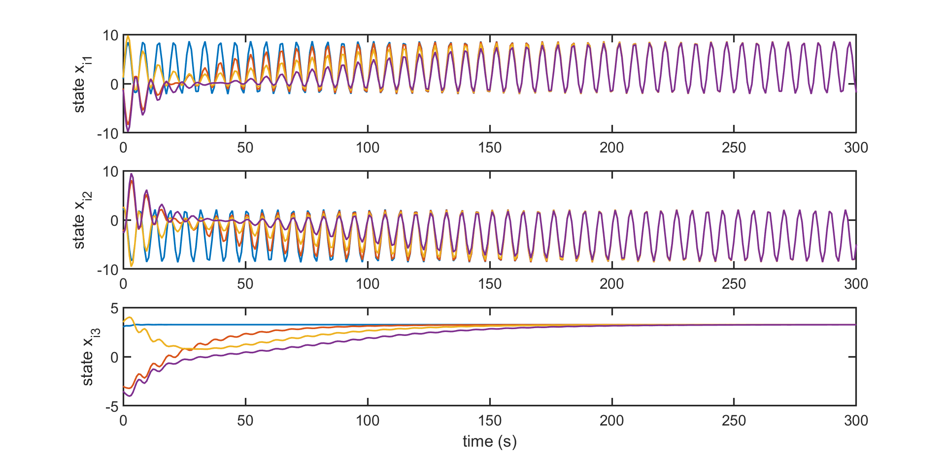
5.4 Synchronization results

The simulation results for both Cases I and II are demonstrated in Fig. 3 and 5. The error between the states $x_{ij}-x_{i1}$ are shown in Fig. 5 to show the synchronization more clearly. The results illustrate that the protocol design is independent of the communication graph and is scale free so that we can achieve synchronization with a one-shot protocol design, for any graph with any number of agents.

6 Conclusion

In this paper we have provided necessary and sufficient conditions for the existence of solutions to the state synchronization problem of homogeneous MAS via scale-free linear dynamic non-collaborative protocols without or with locally bounded neighborhoods for both continuous- and discrete-time. The necessary and sufficient conditions show that the scale-free state synchronization can be achieved for this class of MAS. On the one hand, for continue-time MAS, locally bounded neighborhoods can relax the necessary conditions (i.e., weakly minimum phase and relative degree one). However, there is no linear dynamic design that can remove the condition of neutrally stable. On the other hand, for discrete-time MAS, without locally bounded neighborhood the scale-free design via linear protocols is not possible. However, with locally bounded neighborhoods, we can achieve scale-free synchronization for MAS with neutrally stable agents.

Finally, our result shows that scale-free design via a linear dynamic non-collaborative protocol essentially requires agents to be neutrally stable. However, the paper [10] shows a scale-free design via nonlinear protocol is possible without the neutrally stable condition in the case of full-state coupling. Our future research focuses on obtaining necessary and sufficient conditions for scale-free design via nonlinear protocols for the case of partial-state coupling.

References

[1] H. Bai, M. Arcak, and J. Wen. Cooperative control design: a systematic, passivity-based approach. Communications and Control Engineering. Springer Verlag, 2011.
[2] F. Bullo. Lectures on network systems. Kindle Direct Publishing, 2019.
[3] C. Godsil and G. Royle. Algebraic graph theory, volume 207 of Graduate Texts in Mathematics. Springer-Verlag, New York, 2001.
[4] L. Kocarev. Consensus and synchronization in complex networks. Springer, Berlin, 2013.
[5] J. Lee, J. Kim, and H. Shim. Disc margins of the discrete-time LQR and its application to consensus problem. Int. J. System Science, 43(10):1891–1900, 2012.
[6] Z. Li, Z. Duan, and G. Chen. Consensus of discrete-time linear multi-agent system with observer-type protocols. Discrete and Continuous Dynamical Systems. Series B, 16(2):489–505, 2011.
[7] Z. Li, Z. Duan, G. Chen, and L. Huang. Consensus of multi-agent systems and synchronization of complex networks: A unified viewpoint. IEEE Trans. Circ. & Syst.-I Regular papers, 57(1):213–224, 2010.
[8] Z. Liu, D. Nojavanzedah, and A. Saberi. Cooperative control of multi-agent systems: A scale-free protocol design. Springer, Cham, 2022.
[9] Z. Liu, A. Saberi, and A.A. Stoorvogel. Scale-free non-collaborative linear protocol design for a class of homogeneous multi-agent systems. IEEE Trans. Aut. Contr., 69(5):3333–3340, 2024.
[10] Z. Liu, M. Zhang, A. Saberi, and A. A. Stoorvogel. Leaderless state synchronization of homogeneous multi-agent systems via a universal adaptive nonlinear dynamic protocol. In 2018 Chinese Control And Decision Conference, pages 5–10, Shenyang, China, 2018.
[11] M. Mesbahi and M. Egerstedt. Graph theoretic methods in multiagent networks. Princeton University Press, Princeton, 2010.
[12] R. Olfati-Saber, J.A. Fax, and R.M. Murray. Consensus and cooperation in networked multi-agent systems. Proc. of the IEEE, 95(1):215–233, 2007.
[13] R. Olfati-Saber and R.M. Murray. Consensus problems in networks of agents with switching topology and time-delays. IEEE Trans. Aut. Contr., 49(9):1520–1533, 2004.
[14] W. Ren and R.W. Beard. Consensus seeking in multiagent systems under dynamically changing interaction topologies. IEEE Trans. Aut. Contr., 50(5):655–661, 2005.
[15] W. Ren and Y.C. Cao. Distributed coordination of multi-agent networks. Communications and Control Engineering. Springer-Verlag, London, 2011.
[16] A. Saberi, A. A. Stoorvogel, M. Zhang, and P. Sannuti. Synchronization of multi-agent systems in the presence of disturbances and delays. Birkhäuser, New York, 2022.
[17] S. Stüdli, M. M. Seron, and R. H. Middleton. Vehicular platoons in cyclic interconnections with constant inter-vehicle spacing. In 20th IFAC World Congress, volume 50(1) of IFAC PapersOnLine, pages 2511–2516, Toulouse, France, 2017. Elsevier.
[18] E. Tegling, B. Bamieh, and H. Sandberg. Localized high-order consensus destabilizes large-scale networks. In American Control Conference, pages 760–765, Philadelphia, PA, 2019.
[19] E. Tegling, B. Bamieh, and H. Sandberg. Scale fragilities in localized consensus dynamics. Automatica, 153(111046):1–12, 2023.
[20] E. Tegling, R. H. Middleton, and M. M. Seron. Scalability and fragility in bounded-degree consensus networks. In 8th IFAC Workshop on Distributed Estimation and Control in Networked Systems, volume 52(20), pages 85–90, Chicago, IL, 2019. IFAC-PapersOnLine, Elsevier.
[21] S.E. Tuna. Synchronizing linear systems via partial-state coupling. Automatica, 44(8):2179–2184, 2008.
[22] C.W. Wu. Synchronization in complex networks of nonlinear dynamical systems. World Scientific Publishing Company, Singapore, 2007.

	$\displaystyle\dot{V}_{2}$	$\displaystyle=\tilde{\varphi}^{}(A^{\mbox{\tiny T}}P+PA)\tilde{\varphi}-\delta(1-\lambda)\tilde{\varphi}^{}PBB^{\mbox{\tiny T}}P(e+\tilde{\varphi})-\delta(1-\lambda^{})(e+\tilde{\varphi})^{}PBB^{\mbox{\tiny T}}P\tilde{\varphi}$
		$\displaystyle\leqslant-\delta\|1-\lambda\|^{2}\tilde{\varphi}^{}PBB^{\mbox{\tiny T}}P\tilde{\varphi}-\delta(1-\lambda)\delta\tilde{\varphi}^{}PBB^{\mbox{\tiny T}}Pe-\delta(1-\lambda^{})e^{}PBB^{\mbox{\tiny T}}P\tilde{\varphi}$
		$\displaystyle\leqslant-\tfrac{3}{4}\delta\|1-\lambda\|^{2}\tilde{\varphi}^{}PBB^{\mbox{\tiny T}}P\tilde{\varphi}+4\delta e^{}PBB^{\mbox{\tiny T}}Pe$