The relationship between the turnover frequency and photo-ionisation in radio sources
Abstract
We investigate the connection between the turnover frequency in the radio spectrum, , and the rate of ionising ultra-violet photons, , in extragalactic sources. From a large, optically selected, sample we find to be correlated with in sources which exhibit a turnover. The significance of the correlation decreases when we include power-law radio sources as limits, by assuming that the turnover frequency occurs below the lowest value observed. However, the power-law fit sources are less well sampled across the band and so these may just be contributing noise to the data. Given that the observed – correlation is purely empirical, we use the ionising photon rate to obtain the electron density in a free-free absorption model. For each of the constant, exponential, constant plus exponential (Milky Way) and spherical models of the gas distribution, there is also an increase in the turnover frequency with ionising photon rate. Furthermore, for a given gas mass, we find that the turnover frequency is anti-correlated with the scale-factor of the gas density. While other mechanisms, such as ageing electrons or synchrotron self-absorption, may be required to reproduce the spectral indices, for an exponential scale-factor similar to the linear size, this simple free-free absorption model reproduces the turnover– size correlation seen in radio sources.
keywords:
Radio continuum: galaxies – quasars: general – galaxies: active – galaxies: high-redshift – ultraviolet: galaxies1 Introduction
High-frequency peaked/gigahertz peaked-spectrum (HFP/GPS) and compact steep-spectrum (CSS) sources form a class of radio source which exhibit a peak in their radio spectrum, while the emission appears to be confined to a small region. Specifically HFPs and GPSs have projected linear sizes of kpc and peak in their luminosity at a turnover frequency of GHz, whereas CSSs have kpc and GHz. This reflects the well established anti-correlation between and (Fanti et al., 1990; O’Dea & Baum, 1997; O’Dea, 1998).
The main competing hypotheses for the nature of these are
-
1.
that the more compact sources are young and will evolve into the larger CSSs (Fanti et al., 1995),
-
2.
that all of the sources are due to confinement of the radio jets by a dense interstellar medium (the “frustrated” model, O’Dea et al. 1991),
- 3.
The main issue with the youth argument is the apparent under-abundance of the larger active galactic nucleus (AGN) population into which they canonically evolve (Readhead et al., 1996; O’Dea & Baum, 1997; An & Baan, 2012). However, there is mounting evidence that, in addition to frustrated sources and those which will evolve, many of the “young” sources are transient with their radio activity being cyclic on a time-scale of yr (An & Baan, 2012; Callingham et al., 2015, 2017; O’Dea & Saikia, 2021).
The large rotation measure in some compact radio sources suggests the presence of large magnetic fields (e.g. Kato et al. 1987), indicating that the radio emission is synchrotron in nature (e.g. Bicknell et al. 1997). However, the majority show only weak polarisation (Stanghellini et al., 1998), which may therefore favour free-free absorption as the dominant mechanism (e.g. Marr et al. 2014; Tingay et al. 2015; Keim et al. 2019), although Bicknell et al. suggest that a large number of magnetic field reversals could keep the net polarisation low.
The dominance of the electron density (free-free absorption) is supported by anti-correlation between the neutral gas abundance, as traced through absorption of the 21-centimetre transition of hydrogen (H i), and turnover frequency in 196 radio sources (Curran et al., 2019): The detection rate of H i 21-cm absorption is also strongly anti-correlated with the photo-ionisation rate, , (Curran et al., 2008; Curran & Whiting, 2012). where drives the electron density.
Thus, we were interested to test whether any of the nine quasars, in which only one had evidence of a possible turnover (Gloudemans et al., 2023), have relatively low ionising photon rates. However, sufficient rest-frame ultra-violet photometry was available for only one source, which did in fact have an ionising rate well below the cut-off where neutral gas has ever been detected ( s-1). This is therefore consistent with the argument that no turnover is evident due to a low ionisation rate and, thus, a low electron density.
However, given that this is a single source, to ensure a sample with more comprehensive ultra-violet data, we also searched the photometry of a larger, optically selected sample. From this we find a positive correlation between the turnover frequency and ionising rate, which is supported by a theoretical model. The model also yields an anti-correlation between the turnover frequency and the scale-length of the gas density, which could naturally explain the observed – anti-correlation.
2 The observed correlation
2.1 Photometry and fitting
We follow the same procedure as described in Curran et al. (2013), where the data were scraped from the NASA/IPAC Extragalactic Database (NED)111See Appendix A., the Wide-Field Infrared Survey Explorer (WISE, Wright et al. 2010) Two Micron All Sky Survey (2MASS, Skrutskie et al. 2006) and the Galaxy Evolution Explorer (GALEX, data release GR6/7)222http://galex.stsci.edu/GR6/#mission databases. For the Gloudemans et al. (2023) sources the radio data from NED were supplemented with 54 MHz to 3 GHz photometry from Callingham et al. (2017); Slob et al. (2022); Gloudemans et al. (2022). After shifting the data back into the source’s rest-frame, each flux density measurement, , was then converted to a specific luminosity, via , where is the luminosity distance to the source.333We use km s-1 Mpc-1 and (Planck Collaboration et al., 2020) throughout the paper.
After the removal of duplicate measurements at exactly the same frequency, where there were at least three radio measurements, we applied both log-space first and second order polynomial fits to the data, selecting that which gave the lowest sum residual, , Fig. 1. If there were less than three measurements the source was not used. Note that the 2nd order fit sources which gave a turnover frequency below the minimum observed were re-fitted with a power law.

We used the values from the polynomial as the initial guesses to a GPS-fit function (equation 1 of Snellen et al. 1998). However, due to the limited number of well separated radio photometry points, the bunching of the data at similar frequencies gave much more disparate fits. The polynomial fitting appeared to be more robust, mostly giving reasonable agreement with the GPS-fits, and better agreement with those of O’Dea & Baum (1997).444See Appendix B.
The ionising ( Å) photon rate was determined from the rest-frame UV luminosities, via (Osterbrock, 1989)
| (1) |
where is the frequency (with Hz for H i) and the Planck constant. Again, requiring at least three photometry measurements, fitting the rest-frame UV data with a power-law fit, , gives
| (2) |
where is the log-space intercept and the gradient (the UV spectral index, see Fig. 1). Integrating this over to gives the ionising photon rate as
| (3) |
which was then calculated for each source with sufficient rest-frame UV photometry.
2.2 Samples
2.2.1 The Gloudemans et al. sample
As stated above, only one source, J0002+2550 (WISEA J000239.39+255035.1), had sufficient rest-frame UV data to determine the ionising photon rate.555Of the remaining eight, only four had any rest-frame IR–UV photometry and are shown in Appendix C.

This is shown in Fig. 2, from which we obtain an ionising rate of s-1. This is well below the s-1 limit at which all of the gas in the host galaxy is believed to be ionised (Curran & Whiting, 2012) and well within the regime where H i 21-cm absorption has been detected (Curran et al., 2008, 2019).
Thus, for the one source for which we could obtain the photometry, the absence of a turnover in the radio SED is consistent with a relatively low ionisation fraction. We do note, however, that this has an unusually steep spectral index in the UV band () and whether this applies to the other eight sources in the sample we cannot comment. At such high redshifts we would expect a steepening of the spectral index due to intervening hydrogen, specifically the Lyman- forest (e.g. Janknecht et al. 2002; Barger & Cowie 2010) and Lyman Limits systems (e.g. Mo et al. 2010). In Fig. 2, Å occurs immediately after the second highest frequency point and so the above ionising photon rate should be treated as a lower limit (see Sect. 3.2).
In order to investigate the relation between the ionising photon rate and turnover frequency, we turned to a large sample, which is optically selected in order to increase the likelihood of yielding the necessary rest-frame UV photometry.
2.2.2 The SDSS sample
We use the sample of Curran et al. (2021), which comprises the first 100 000 QSOs of the SDSS Data Release 12 (DR12, Alam et al. 2015) with accurate redshifts. From these we shortlisted the sources which had at least one flux measurement below 10 GHz, giving 3429 radio sources. As stated above, we required at least three flux measurements to fit the radio data, which gave 1005 sources of which 499 could be fit. Of these, the ionising photon rate could be obtained for 416 source, of which 257 sources which were fit by a power law with 159 exhibiting a turnover. Since we are primarily interested in the turnover frequency, we used the polynomial results in the following analysis.
In order to supplement the radio data, we added photometry compiled in surveys with the GaLactic and Extragalactic All-sky Murchison Widefield Array (GLEAM), specifically:
-
1.
The 1483 sources with Mz (Callingham et al., 2017).
-
2.
The 373 sources of Slob et al. (2022), of which 36 exhibit Mz.
-
3.
The 24 high redshift () radio bright sources of Gloudemans et al. (2022).
Of the first two samples, spectroscopic redshifts were available for 214 and 49 sources, respectively. Comparing these with the SDSS sample gave just a single match, [HB89] 1252+119 (GLEAM J125438+114103) at .666Note that there are two other coordinate matches, [HB89] 1307+121 (GLEAM J130934+115425) and [HB89] 1442+101 (GLEAM J144516+095835), although the redshifts of the SDSS and GLEAM sources are very different – , cf. 0.34286 and , cf. 0.25578, respectively. The lowest observed rest-frame frequency is 141 MHz, compared to 676 MHz for the NED only data. For the low frequency plus NED photometry, the polynomial fit gives Hz = GHz and the GPS fit 251 MHz (Fig. 3), whereas the NED only data gives Hz = MHz and the GPS fit 603 MHz777Which, being lower than the minimum observed frequency, would be re-fitted with a power law.. This is actually closer to the MHz of Callingham et al. (2017)888325 MHz in the observed frame (J. Callingham, private communication). which uses the low frequency data.

2.2.3 The low frequency samples
We also performed full photometry searches on the low frequency samples. Of the sources with at least three radio photometry measurements, 260 have spectroscopic redshifts, of which 24 were best fit by a power law and 201 with a turnover.999Although the remaining 35 appeared to be amply sampled, some gave inverted spectra and the bunching of data at similar frequencies in others prevented a fit. Just 55 of these had sufficient rest-frame UV photometry to obtain the ionising photon rate and adding these to the SDSS sources with a measured , gave 263 first order fit sources and 208 second order fit.
2.3 Selection effects
2.3.1 Radio flux limits
In Fig. 4 we show the radio and UV luminosity distributions of the combined SDSS plus low frequency sample.

The UV and radio luminosities are strongly correlated, with a Kendall-tau test giving a probability of of this arising by chance, which is significant at , assuming Gaussian statistics. Also, it is apparent that the 1st order fit sources are generally more luminous at cm than those with a 2nd order fit.
This could be due to the flagging of 2nd order fits as 1st order if the fitted turnover frequency is below the minimum observed, which will have the effect of boosting the luminosity if the putative turnover occurs at GHz. This may be evident in Fig. 5, where

the 2nd order fit sources are, on average, more fully sampled, thus making it possible that some of the 1st order fit sources may exhibit a turnover if sampled to a similar degree. The median radio bandwidths of the low frequency observations is MHz (Callingham et al., 2017; Slob et al., 2022) and so we remove our most extreme outliers (at GHz) from the sample in the following analysis.
2.3.2 UV photometry correction
As discussed in Sec. 2.2.1, the higher the redshift the more we expect the rest-frame UV continuum to be absorbed by intervening hydrogen.

In the top panel of Fig. 6, we can see a clear Malmquist bias, where the volume probed at low redshift is insufficient to detect the rare high luminosity sources, while at high redshift only the high luminosity sources are detected. We therefore use the spectral index to quantify a correction for the intervening hydrogen. In Fig. 7 we show all of the SDSS sources for which we could obtain an ionising photon rate,

from which we can see a steepening in the spectral index with redshift. A linear fit gives , so, on the basis that the intrinsic spectral index is at , we correct each measured value of by subtracting (Fig. 8).101010 at is similar to values in the literature, e.g. at (Shull et al., 2012) and at (Telfer et al., 2002).

Although not valid for an individual source, using this to correct the UV spectral index to obtain the intrinsic value provides a statistical correction for the redshift, and thus a better estimate of the ionising photon rate before the absorption of the UV continuum by intervening gas.111111There is also the issue of dust suppressing the shorter wavelengths in the rest-frame, leading to underestimates in . However, intrinsic dust will also provide shielding for the gas countering the degree of ionisation somewhat.
2.4 Ionising photon rate and turnover frequency
2.4.1 Correlations
From the corrected spectral indices we recalculate the ionising photon rates, according to Equ. 3. Showing these in Fig. 9,
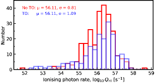
we see little difference between the 1st and 2nd order fit sources. A -test gives a probability of of the mean values being the same and a Kolmogorov-Smirnov test gives of the populations being drawn from the same sample.121212For the uncorrected ionising photon rates these are and .
In Fig. 10 we show the turnover frequency versus the ionising photon rate,


from which we see a correlation between and , which has a probability of arising by chance. Given this correlation, we now assume that the sources which exhibit no turnover have not been searched to sufficiently low frequencies. We include these sources by assigning the lowest observed rest-frame frequency as the upper limit to this (e.g. Fanti et al. 1990). We also apply this to the 2nd order fit sources where the turnover frequency yielded by the fit is lower than the lowest observed rest-frame frequency (Fig. 11).

In order to incorporate the limits, we use the Astronomy SURVival Analysis (asurv) package (Isobe et al., 1986) which adds these as censored data points, allowing a generalised non-parametric Kendall-tau test. Including these weakens the correlation ()131313For the uncorrected ionising photon rates this is ()., which may suggest, if , that the 1st order fit sources are not dominated by those which have not been searched to low enough frequencies to detect the turnover. However, given the lower frequency ranges of the 1st order fit sources (Sect. 2.3.1), the detection of a turnover if the sampling were ample cannot be ruled out. Hence, it is also possible that the inclusion of these sources only acts to introduce noise.
2.4.2 Caveats
While we have found a strong correlation between the turnover frequency and the ionising photon rate, one should be aware of:
-
1.
For the one SDSS source which did match the low frequency catalogues, the lowest rest-frame frequency yielded by NED was 676 MHz, compared to 141 MHz from the low frequency data (Sect. 2.2.2). Thus, until observed and included in NED, allowing automated photometry scraping, it is reasonable to assume that many of the SDSS (1st order fit) sample have not been observed to sufficiently low frequencies.
-
2.
The 1st order fit sources generally have sparser sampling across the radio band (Sect. 2.3.1). So, until the power-law sources are sampled as comprehensively as those exhibiting a turnover, we cannot be certain that a potential turnover does not occur within the observed range.
-
3.
As seen in Fig. 10, there is a large variation in the uncertainties in the turnover frequencies. Two examples, at either end of the range, are shown in Fig. 12.


Figure 12: Left: Example of a low uncertainty in the turnover frequency, with from 25 photometry points. Right: Example of a high uncertainty, with from nine photometry points. In a large enough sample we expect as may overestimates as underestimates, so that the biases introduced by these would be largely averaged out. Ideally, however, these should all be small and so, again, more comprehensive sampling of the radio band is required.
-
4.
From the upper limits in Fig. 11, we see that the lowest observed frequency is correlated with the ionising photon rate, which is most likely driven by the redshift, where sources are observed to the same minimum frequency in a given survey, confirmed in Fig. 13.

Figure 13: The rest-frame minimum observed frequencies versus redshift. This is also evident in Gloudemans et al. (2023), where the high redshifts () cause the low observed frequencies ( GHz) to be insensitive to turnover frequencies below GHz.
3 Modelling the correlation
3.1 Dependence of the turnover frequency on the photo-ionisation rate
We have found a correlation between the turnover frequency and the ionising photon rate (Fig. 10). Although this supports the hypothesis that there is a connection between the turnover frequency and ionising photon rate it is an empirical result. To explore the cause of the correlation we now examine the theoretical dependence between the turnover frequency, as caused by free-free absorption, and the number of photons available to ionise the neutral atomic gas.
For free-free radiation the absorption coefficient is
| (4) |
where is the atomic number, the electronic charge, the electron density, the Boltzmann constant, the temperature, the permittivity of free space, the speed of light and the electron mass.
For neutral hydrogen (), this can be written as
| (5) |
per metre, where is in .
For a spherical H ii region of radius , at a luminosity distance , the flux density is
| (6) |
where for a sphere of constant density, the optical depth is and is the specific brightness, which, in the Rayleigh-Jeans regime () is given by
| (7) |
In equilibrium, the rate of ionisation is balanced by the rate of recombination (Osterbrock, 1989),
| (8) |
where is the proton density and the radiative recombination rate coefficient of hydrogen ( cm3 s-1 at the canonical K, Osterbrock & Ferland 2006).141414http://amdpp.phys.strath.ac.uk/tamoc/DATA/RR/
3.1.1 Constant density profile
From Equ. 8, the ionising photon rate required to completely ionise a neutral plasma () of constant density within a Strömgren sphere of radius is
| (9) |
For a range of ionising photon rates we use this to obtain the electron density, which we insert into Equ. 5, giving the absorption coefficient . For a constant electron density through a path , which, via Equ. 6, gives the variation in flux density with frequency (Fig. 14).

From this, it is clear that for a given density, temperature and radius, the turnover frequency is correlated with the ionising photon rate, as is seen for the observational data (Sect. 2.4.1).
3.1.2 Exponential density profile
A more physically realistic model, especially on galactic scales, is an exponential decrease in gas density with distance from the nucleus of the galaxy (e.g. Baldwin 1982; Begeman et al. 1991). O’Dea & Baum (1997) use a distribution of the form , where . However, this gives at and an infinite column density for . We therefore use the exponential sphere model, , which gives .
Using the Milky Way’s and breaking the degeneracy via the gas mass (Curran & Whiting, 2012)
| (10) |
where is the Galactic flare factor (Kalberla & Kerp, 2009), gives M⊙, and kpc for the Milky Way (Fig. 15).

For the exponential sphere complete ionisation of the gas occurs when the ionising photon rate reaches (Curran & Whiting, 2012)
| (11) |
Using Equ. 11 to obtain for a given , where the gas is completely ionised (Fig. 16),

gives the optical depth through the gas as (Equ. 5)
Integrating this gives
| (12) |
which, again via Equ. 6, gives the variation in flux density with frequency (Fig. 17, left). Like the constant density distribution, this exhibits an increase in the turnover frequency with ionising photon rate.

Although, unlike the constant density model, at large distances the path length is not required for the optical depth calculation, a value is required for the flux density (Equ. 6) and we have assumed that as the extent over which the emission can be detected. However, while the flux densities are not absolute, the turnover frequency is independent of the choice of .
3.1.3 Constant and exponential density (compound) profile
For the Milky Way the gas distribution is a combination of both the constant and exponential profile (Kalberla & Kerp, 2009);
where , kpc and kpc (see Fig. 15). For this distribution complete ionisation of the gas occurs when the ionising photon rate is (Curran, 2024)
| (13) |
Again, assuming that all of the gas is ionised, we use the electron density for a given ionising photon rate (Equ. 13) to calculate the optical depth through the gas
which gives
| (14) |
This results in the frequency profiles shown in Fig. 17 (middle), where, again, we have assumed as the size of the emission region, although this does not affect the apparent correlation.
3.1.4 Elliptical profiles
Since our sample comprises radio loud AGN, it is likely that most of the host galaxies are elliptical. These can be modelled via several similar density profiles, e.g. the Jaffe profile (Jaffe, 1983), which models the distribution of light in a spherical galaxy as , where is the radius which contains half the total emitted light. However, as seen in Fig. 18 this has an asymptotic density distribution, as does the NFW profile (Navarro et al., 1996), , where is the radius of the halo core.

These can be avoided by employing the halo density distribution of an isothermal sphere, for example (Begeman et al., 1991) or equation 7 of Capelo et al. (2010),
where is the gravitational constant, is the critical density of the Universe is a scale radius, the mean molecular weight of the gas and the proton mass. We select this, the simplest model, cf. the polytropic and stellar models, to limit the number of free parameters. Using the column density of the Milky Way at kpc ( ) to constrain the characteristic density gives for K and .
Given its relative simplicity, while yielding a similar density profile to that of Capelo et al. (2010), we use the profile of Begeman et al., for which complete ionisation of the gas occurs when
Proceeding as above, the optical depth through the completely ionised gas is
giving
| (15) |
which has a similar form to the exponential density (Equ. 12) and frequency (Fig. 17, right) profiles.
3.1.5 Summary
For all of the above models , although there is some variation in the constant of proportionality and each model therefore predicts quite different values for the turnover frequency,
| [s-1] | Gas density model | |||
|---|---|---|---|---|
| Constant | Exponential | Compound | Iso. Sphere | |
| 11 MHz | 1.9 MHz | 8.5 MHz | 1.0 MHz | |
| 35 MHz | 5.6 MHz | 25 MHz | 2.9 MHz | |
| 100 MHz | 16 MHz | 74 MHz | 8.7 MHz | |
| 300 MHz | 49 MHz | 220 MHz | 26 MHz | |
| 0.89 GHz | 140 MHz | 0.65 GHz | 76 MHz | |
| 2.6 GHz | 0.43 GHz | 1.9 GHz | 0.22 GHz | |
| 8.8 GHz | 1.3 GHz | 5.5 GHz | 0.66 GHz | |
which can vary by up to an order of magnitude for a given ionising rate (Table 1). Only where there is a constant density component, will we see a turnover at GHz for s-1 (sufficient to ionise all of the gas in a large spiral). For the exponential and spherical models it appears that s-1 is required for GHz, which is consistent with the hypothesis that sources with no turnover are not subject to complete ionisation.
3.2 The turnover frequency of J0002+2550
Equipped with the expected value of the turnover frequency for a given photo-ionisation rate, we can estimate the turnover for J0002+2550 (Sect. 2.2.1). At , the luminosity distance to the source is Mpc and the finest beam size of , in which the source is unresolved (Gloudemans et al., 2023), gives kpc for the low frequency emission.
Again, assuming complete ionisation by the observed s-1 (Sect. 2.2.1), in Fig. 19 we show the expected radio SED for various scale-lengths

from which it is apparent that, for a scale-length of kpc, the turnover frequency is GHz. Although consistent with the absence of a turnover at GHz, our simple free-free radiation model (which forces and ) does not trace the steep spectral index of the optically thin portion of the Gloudemans et al. spectrum (where ), which they attribute to the ionised medium producing synchrotron emission in addition to a spectral break caused by ageing electrons.
We note that the predicted flux density approaches the observed mJy at GHz, for a scale length of pc. This is about an order of magnitude lower than that of the Galaxy but, due to hierarchical build-up, we expect smaller galaxies (Baker et al., 2000; Lanfranchi & Friaça, 2003) and, thus, smaller scale-lengths at high redshift. However, we have set the extent of the emission to the minor axis of the smallest beam in which the source is unresolved, and so there is some wriggle room in the absolute flux measurements.
Correcting the UV spectral index for J0002+2550 gives , which results in an ionising photon rate of s-1, which changes little from the uncorrected value. From Table 1, we see that the exponential and spherical gas density profiles allow for no turnover at GHz for relatively high ionising rates ( s-1), whereas the constant density model precludes this at s-1. Unfortunately, the other targets of Gloudemans et al. have insufficient rest-frame UV photometry to see if such steep UV spectra apply to the sample as a whole (see Appendix C). As it is, this source is consistent with a low level of ionisation causing shifting the turnover frequency to below the minimum observed value, but with the caveat that the photometry correction for intervening absorption is statistical only.
3.3 Turnover frequency and size
3.3.1 Observations
As stated in Sect. 1, the turnover frequency is anti-correlated with the projected linear size, which is clearly evident in the O’Dea & Baum (1997) data (Fig. 20).151515 is calculated using updated spectroscopic redshifts and cosmological parameters (Planck Collaboration et al., 2020).

On average, the turnover frequencies we derive are slightly lower than those of O’Dea & Baum, which could be due to the recent increase in the availability of low frequency data (see Appendix B). Out of the 66 sources with a measured linear size, 38 exhibit a turnover, 27 are flagged as upper limits, since the fit gives a turnover below the lowest observed frequency, and one has an inverted spectrum (FBQS J133037.6+250910). Including the limits, and excluding J1330+2509, we obtain for the correlation, which is similar to that using the values of O’Dea & Baum directly, where there are no limits.161616 ().
3.3.2 Model
If the extent of the radio emission scales with , the anti-correlation between turnover frequency and size is evident from our model. Furthermore, for an ionising photon rate of s-1 (J0002+2550, Fig. 19) and , the model is in agreement with the observations (Sect. 1); that is, GHz for kpc (HFPs/GPSs) and GHz for kpc (CSSs).
In order to generalise this, we need to break the degeneracy between and in Equ. 12. For this we use the exponential model for which we can use the fact that, for a given mass, the product is constant (Equ. 10).171717For the spherical model (Sect. 3.1.4), . From a low-redshift survey of 21-cm emission from the 1000 H i brightest galaxies in the southern sky, Koribalski et al. (2004) find a range of M⊙, with a median of M⊙. Using these masses and assuming the Galactic flare factor, for a given scale-length we determine , which is then used in Equs. 12 and 6 to produce an SED (as for Fig. 19), from which we obtain the turnover frequency.181818In Equ. 6, and are only required to obtain the absolute flux density.

The results are shown in Fig. 21, where we see the predictions overlap the observations of O’Dea & Baum (1997) for the range of gas masses expected (assuming ). We also note that the median gas mass of M⊙ passes close to the middle of the distribution of the observed data. This is also closely aligned with the two models of O’Dea & Baum, which are based on synchrotron self-absorption models. Thus, for a gas scale-length close to the radio source size, our simple free-free model can reproduce the observed – relationship.
Lastly, we note that, while we are considering the ionisation of the large-scale gas, the material causing the turnover in the radio SED may be mainly located within the central kpc (e.g. Dallacasa et al. 2000; Callingham et al. 2015; Maccagni et al. 2018). However, for the exponential and isothermal sphere models of the gas density, we see that at 100 MHz the absorption is already optically thick within this region (Fig. 22).

3.4 Ionising photon rates of the O’Dea & Baum sample
Of the O’Dea & Baum sample, only 11 sources have sufficient rest-frame photometry to yield an ionising photon rate, comprising five with a turnover within the sampled frequency range and six without.
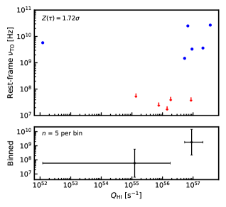
As seen from Fig. 23, five detections and six limits are insufficient to yield a convincing correlation (), although one is suggested by the binning.
4 Discussion and conclusions
It has long been known that the turnover frequency in the SEDs of extragalactic radio sources is anti-correlated with the projected size of the emission. If the profile of the radio SED is dominated by free-free absorption we way may expect the turnover frequency, , to be related to the rate of ionising photons emitted by the AGN. Thus, we suggest that radio sources which do not exhibit a turnover have low ionising photon rates, causing the turnover to be below the minimum observed frequency.
To test this, we initially examined the observational data, mining all of the radio, IR, optical and UV photometry, in order to obtain the turnover frequency and ionising photon rate:
-
•
For the sample of Gloudemans et al. (2023), where only one of the nine high redshift sources shows any indication of a turnover: Sufficient rest-frame UV photometry was available for only one source, J0002+2550. This was found to have a relatively low ionising photon rate of s-1, which is consistent with a low turnover frequency.
-
•
For a larger sample, optically selected in order to increase the number of sources with comprehensive UV photometry:
-
–
For the sources which exhibit a turnover in their radio SED, we find a correlation between and , significant at .
-
–
By assuming that the radio sources fit by a power-law have their turnover frequencies below the minimum observed, the significance reduces to . However, there is strong evidence that the power-law sources are not as comprehensively sampled in the radio band than those exhibiting a turnover, and, if these do have a putative undetected peak in the spectrum, including these adds noise to the data. Thus, more complete sampling in the radio band for the power-law sources is required.
-
–
While compelling, the correlation between the turnover frequency and the ionising photon rate is an empirical result and so, to provide a physical justification, we produced a model relating to , via the electron density. This is done by assuming purely free-free radiation from a completely ionised galactic disk/sphere. From this we find;
-
•
For gas of a constant density, an exponential density profile, a combination of both (as per the Milky Way) and a spherical density profile, that the turnover frequency is correlated with ionising photon rate, which must exceed that to ionise all of the gas in a large spiral ( s-1) in order to exhibit GHz. This supports the hypothesis that sources with low ionising photon rates ( s-1) have their turnover frequencies below the minimum observed ( GHz)
-
•
That the exponential and spherical density models can fit the SED of J0002+2550 for pc, suggesting that the turnover frequency is indeed below the lowest observed rest-frame frequency of 1 GHz.
-
•
For a given mass of neutral gas, and using the scale-length as a proxy for the projected linear size, the dependence of turnover frequency on the scale-length of the exponential gas distribution closely traces the observational data and the synchrotron self-absorption model.
The model, which relies solely on ionisation of the atomic gas by the AGN, is considerably simpler than the synchrotron self-absorption models (Bicknell et al., 1997; O’Dea & Baum, 1997), which have to assume a large number of magnetic field reversals to keep net polarisation at the low values which are observed.
However, given the sparseness of the radio data, when prioritising sources with measured UV luminosities, we cannot reliably determine spectral indices below and above the turnover. A further caveat is we assume that the gas is completely ionised, although the fact that all of the distributions tested give the same dependence may suggest that the model remains valid over a region of ionisation enclosed within an envelope of neutral gas. We also assume that the scale-length of the gas distribution is proportional to the extent the emission. This is a reasonable assumption and only affects the flux density of the modelled source and not the turnover frequency. Interestingly, setting the scale-length does reproduce the – synchrotron self-absorption models (O’Dea & Baum, 1997) for the median gas mass ( M⊙).
Future wide-field spectroscopy of radio sources, including those of the low frequency sample, e.g with WEAVE (Dalton et al., 2012; Smith et al., 2016), will allow us to determine many more ionising photon rates for the sources which have been observed to considerably lower frequencies than the SDSS sample. These will prove invaluable in determining whether the power-law sources have simply not been observed to sufficiently low frequencies, as posited here. With a large number of sources probed to very low frequencies, we may also be able to constrain which gas distribution best follows the model and perhaps yield an estimate of the ionising photon rate in the absence of observed frame UV-optical-IR photometry. A strong anti-correlation between the abundance of cool neutral gas and the ionising photon rate has been long established (Curran et al., 2008; Curran, 2024) and, in the absence of observationally expensive follow-up UV photometry, it will be interesting to see if the turnover frequency is also anti-correlated with the detection of H i absorption from ongoing and future surveys with the SKA and its pathfinders, e.g. the First Large Absorption Survey in H i (FLASH, Allison et al. 2022).
Data availability
Data available on request and the NED photometry data are included in the online versions.
Acknowledgements
I would like to thank the anonymous referee and the scientific editors, Tim Pearson, for their helpful and constructive comments which helped improve the manuscript. This research has made use of the NASA/IPAC Extragalactic Database (NED) which is operated by the Jet Propulsion Laboratory, California Institute of Technology, under contract with the National Aeronautics and Space Administration and NASA’s Astrophysics Data System Bibliographic Service. This research has also made use of NASA’s Astrophysics Data System Bibliographic Service and asurv Rev 1.2 (Lavalley et al., 1992), which implements the methods presented in Isobe et al. (1986).
References
- Alam et al. (2015) Alam S. et al., 2015, ApJS, 219, 12
- Allison et al. (2022) Allison J. R. et al., 2022, PASA, 39, e010
- An & Baan (2012) An T., Baan W. A., 2012, ApJ, 760, 77
- Bañados et al. (2014) Bañados E. et al., 2014, AJ, 148, 14
- Baker et al. (2000) Baker A. C., Mathlin G. P., Churches D. K., Edmunds M. G., 2000, in Star Formation from the Small to the Large Scale, Vol.45 of ESA SP, Favata F., Kaas A., Wilson A., eds., ESA Special Publication, Noordwijk, p. 21
- Baldwin (1982) Baldwin J. E., 1982, in Extragalactic Radio Sources, Heeschen D. S., Wade C. M., eds., Vol. 97, pp. 21–24
- Barger & Cowie (2010) Barger A. J., Cowie L. L., 2010, ApJ, 718, 1235
- Begelman (1999) Begelman M. C., 1999, in The Most Distant Radio Galaxies, Röttgering H. J. A., Best P. N., Lehnert M. D., eds., p. 173
- Begeman et al. (1991) Begeman K. G., Broeils A. H., Sanders R. H., 1991, MNRAS, 249, 523
- Bicknell et al. (1997) Bicknell G. V., Dopita M. A., O’Dea C. P. O., 1997, ApJ, 485, 112
- Callingham et al. (2017) Callingham J. R. et al., 2017, ApJ, 836, 174
- Callingham et al. (2015) Callingham J. R. et al., 2015, ApJ, 809, 168
- Capelo et al. (2010) Capelo P. R., Natarajan P., Coppi P. S., 2010, MNRAS, 407, 1148
- Curran (2024) Curran S. J., 2024, PASA, 41, 7
- Curran et al. (2019) Curran S. J., Hunstead R. W., Johnston H. M., Whiting M. T., Sadler E. M., Allison J. R., Athreya R., 2019, MNRAS, 484, 1182
- Curran et al. (2021) Curran S. J., Moss J. P., Perrott Y. C., 2021, MNRAS, 503, 2639
- Curran & Whiting (2012) Curran S. J., Whiting M. T., 2012, ApJ, 759, 117
- Curran et al. (2013) Curran S. J., Whiting M. T., Sadler E. M., Bignell C., 2013, MNRAS, 428, 2053
- Curran et al. (2008) Curran S. J., Whiting M. T., Wiklind T., Webb J. K., Murphy M. T., Purcell C. R., 2008, MNRAS, 391, 765
- Dallacasa et al. (2000) Dallacasa D., Stanghellini C., Centonza M., Fanti R., 2000, A&A, 363, 887
- Dalton et al. (2012) Dalton G. et al., 2012, in Society of Photo-Optical Instrumentation Engineers (SPIE) Conference Series, Vol. 8446, Ground-based and Airborne Instrumentation for Astronomy IV, McLean I. S., Ramsay S. K., Takami H., eds., p. 84460P
- Fanti et al. (1995) Fanti C., Fanti R., Dallacasa D., Schilizzi R. T., Spencer R. E., Stanghellini C., 1995, A&A, 302, 317
- Fanti et al. (1990) Fanti R., Fanti C., Schilizzi R. T., Spencer R. E., Nan Rendong, Parma P., van Breugel W. J. M., Venturi T., 1990, A&A, 231, 333
- Gloudemans et al. (2022) Gloudemans A. J. et al., 2022, A&A, 668, A27
- Gloudemans et al. (2023) Gloudemans A. J. et al., 2023, A&A, 678, A128
- Isobe et al. (1986) Isobe T., Feigelson E., Nelson P., 1986, ApJ, 306, 490
- Jaffe (1983) Jaffe W., 1983, MNRAS, 202, 995
- Janknecht et al. (2002) Janknecht E., Baade R., Reimers D., 2002, A&A, 391, L11
- Kalberla & Kerp (2009) Kalberla P. M. W., Kerp J., 2009, Ann. Rev. Astr. Ap., 47, 27
- Kaplan & Meier (1958) Kaplan E. L., Meier P., 1958, J. Amer. Statist. Assoc., 53, 457
- Kato et al. (1987) Kato T., Tabara H., Inoue M., Aizu K., 1987, Nat, 329, 223
- Keim et al. (2019) Keim M. A., Callingham J. R., Röttgering H. J. A., 2019, A&A, 628, A56
- Koribalski et al. (2004) Koribalski B. S. et al., 2004, AJ, 128, 16
- Lanfranchi & Friaça (2003) Lanfranchi G. A., Friaça A. C. S., 2003, MNRAS, 343, 481
- Lavalley et al. (1992) Lavalley M. P., Isobe T., Feigelson E. D., 1992, in BAAS, Vol. 24, pp. 839–840
- Maccagni et al. (2018) Maccagni F. M., Morganti R., Oosterloo T. A., Oonk J. B. R., Emonts B. H. C., 2018, A&A, 614, A42
- Marr et al. (2014) Marr J. M., Perry T. M., Read J., Taylor G. B., Morris A. O., 2014, ApJ, 780, 178
- Mo et al. (2010) Mo H., van den Bosch F. C., White S., 2010, Galaxy Formation and Evolution. Cambridge University Press, Cambridge
- Navarro et al. (1996) Navarro J. F., Frenk C. S., White S. D. M., 1996, ApJ, 462, 563
- O’Dea (1998) O’Dea C. P., 1998, PASP, 110, 493
- O’Dea & Baum (1997) O’Dea C. P., Baum S. A., 1997, AJ, 113, 148
- O’Dea et al. (1991) O’Dea C. P., Baum S. A., Stanghellini C., 1991, ApJ, 380, 66
- O’Dea & Saikia (2021) O’Dea C. P., Saikia D. J., 2021, ARA&A, 29, 3
- Osterbrock (1989) Osterbrock D. E., 1989, Astrophysics of Gaseous Nebulae and Active Galactic Nuclei. University Science Books, Mill Valley, California
- Osterbrock & Ferland (2006) Osterbrock D. E., Ferland G. J., 2006, Astrophysics of Gaseous Nebulae and Active Galactic Nuclei. University Science Books, Sausalito, California
- Planck Collaboration et al. (2020) Planck Collaboration et al., 2020, A&A, 641, A6
- Readhead et al. (1996) Readhead A. C. S., Taylor G. B., Pearson T. J., Wilkinson P. N., 1996, ApJ, 460, 634
- Shull et al. (2012) Shull J. M., Stevans M., Danforth C. W., 2012, ApJ, 752, 162
- Skrutskie et al. (2006) Skrutskie M. F. et al., 2006, AJ, 131, 1163
- Slob et al. (2022) Slob M. M., Callingham J. R., Röttgering H. J. A., Williams W. L., Duncan K. J., de Gasperin F., Hardcastle M. J., Miley G. K., 2022, A&A, 668, A186
- Smith et al. (2016) Smith D. J. B. et al., 2016, in SF2A-2016: Proceedings of the Annual meeting of the French Society of Astronomy and Astrophysics, Reylé C., Richard J., Cambrésy L., Deleuil M., Pécontal E., Tresse L., Vauglin I., eds., pp. 271–280
- Snellen et al. (1998) Snellen I. A. G., Schilizzi R. T., de Bruyn A. G., Miley G. K., Rengelink R. B., Roettgering H. J., Bremer M. N., 1998, A&AS, 131, 435
- Stanghellini et al. (1998) Stanghellini C., O’Dea C. P., Dallacasa D., Baum S. A., Fanti R., Fanti C., 1998, A&AS, 131, 303
- Telfer et al. (2002) Telfer R. C., Zheng W., Kriss G. A., Davidsen A. F., 2002, ApJ, 565, 773
- Tingay et al. (2015) Tingay S. J. et al., 2015, AJ, 149, 74
- Wright et al. (2010) Wright E. L. et al., 2010, AJ, 140, 1868
Appendices
A: NED photometry
The NED photometry for each of our samples are included online in the files SDSS_NED-fluxes.txt (the SDSS sample), G23_NED-fluxes.txt (the Gloudemans et al. sample) and Low-sample_NED-fluxes.txt. These are in the format
No NED1        NED2             z   log10(Freq) log10(Flux)
1  SDSS J205212.82+001137.4 0.6864645 15.29        -4.82
1  SDSS J205212.82+001137.4 0.6864645 15.29        -4.92
1  SDSS J205212.82+001137.4 0.6864645 15.29        -4.83
1  SDSS J205212.82+001137.4 0.6864645 15.13        -4.67
1  SDSS J205212.82+001137.4 0.6864645 15.11        -4.72
where the source number is followed by the NED name, the redshift and of the observed frequency (Hz) and flux (Jy). Note that Low-sample_NED-fluxes.txt has an additional field designating the reference for the source: C17 – Callingham et al. (2017), G22 – Gloudemans et al. (2022), S22 – Slob et al. (2022).
B: The O’Dea & Baum sample
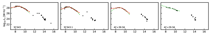
In Fig. 24 we show the SEDs of O’Dea & Baum (1997) with our fits to the UV (Sect. 2.1) and radio (Sect. 2.1) photometry.


In Fig. 25 we show the turnover frequencies obtained from our fits compared to those of O’Dea & Baum (1997).


C: The Gloudemans et al. sample
In addition to Fig. 2, we show in Fig. 26 the photometry scraped from NED, WISE, 2MASS and GALEX for the sources of Gloudemans et al. (2023). Note that for the remaining four sources no photometric data were available.

