The Regulated NiCu Cycles with the new ⁵⁷Cu(p, $\gamma$ )⁵⁸Zn reaction rate and
the Influence on Type-I X-Ray Bursts: GS 1826 $-$ 24 Clocked Burster

Yi Hua Lam (藍乙華) Institute of Modern Physics, Chinese Academy of Sciences, Lanzhou 730000, People’s Republic of China School of Nuclear Science and Technology, University of Chinese Academy of Sciences, Beijing 100049, People’s Republic of China Ning Lu (盧寧) Institute of Modern Physics, Chinese Academy of Sciences, Lanzhou 730000, People’s Republic of China School of Nuclear Science and Technology, University of Chinese Academy of Sciences, Beijing 100049, People’s Republic of China School of Nuclear Science and Technology, Lanzhou University, Lanzhou 730000, People’s Republic of China Alexander Heger School of Physics and Astronomy, Monash University, Victoria 3800, Australia OzGrav-Monash – Monash Centre for Astrophysics, School of Physics and Astronomy, Monash University, VIC 3800, Australia Center of Excellence for Astrophysics in Three Dimensions (ASTRO-3D), VIC 3800, Australia The Joint Institute for Nuclear Astrophysics, Michigan State University, East Lansing, MI 48824, USA Adam Michael Jacobs The Joint Institute for Nuclear Astrophysics, Michigan State University, East Lansing, MI 48824, USA Department of Physics and Astronomy, Michigan State University, East Lansing, MI 48824, USA Nadezda A. Smirnova CENBG, CNRS/IN2P3 and University of Bordeaux, Chemin du Solarium, 33175 Gradignan cedex, France Teresa Kurtukian Nieto CENBG, CNRS/IN2P3 and University of Bordeaux, Chemin du Solarium, 33175 Gradignan cedex, France Zac Johnston The Joint Institute for Nuclear Astrophysics, Michigan State University, East Lansing, MI 48824, USA Department of Physics and Astronomy, Michigan State University, East Lansing, MI 48824, USA Shigeru Kubono (久保野茂) RIKEN Nishina Center, 2-1 Hirosawa, Wako, Saitama 351-0198, Japan Center for Nuclear Study, University of Tokyo, 2-1 Hirosawa, Wako, Saitama 351-0198, Japan

(Received July 23, 2021; Accepted January 14, 2022)

Abstract

During the X-ray bursts of GS 1826 $-$ 24, “clocked burster’, the nuclear reaction flow that surges through the rapid-proton capture process path has to pass through the NiCu cycles before reaching the ZnGa cycles that moderate the further extent of hydrogen burning in the region above germanium and selenium isotopes. The ⁵⁷Cu(p, $\gamma$ )⁵⁸Zn reaction located in the NiCu cycles plays an important role in influencing the burst light curves as found by Cyburt et al. (2016). We deduce the ⁵⁷Cu(p, $\gamma$ )⁵⁸Zn reaction rate based on the experimentally determined important nuclear structure information, isobaric-multiplet-mass equation, and large-scale shell model calculations. Based on the isobaric-multiplet-mass equation, we propose a possible order of $1^{+}_{1}$ and $2^{+}_{3}$ dominant resonance states and constrain the resonance energy of the $1^{+}_{2}$ state. The latter reduces the contribution of the $1^{+}_{2}$ dominant resonance state. The new reaction rate is up to a factor of four lower than the Forstner et al. (2001) rate recommended by JINA REACLIB v2.2 at the temperature regime sensitive to clocked bursts of GS 1826 $-$ 24. Using the simulation from the one-dimensional implicit hydrodynamic code, Kepler, to model the thermonuclear X-ray bursts of GS 1826 $-$ 24 clocked burster, we find that the new ⁵⁷Cu(p, $\gamma$ )⁵⁸Zn coupled with the latest ⁵⁶Ni(p, $\gamma$ )⁵⁷Cu and ⁵⁵Ni(p, $\gamma$ )⁵⁶Cu reaction rates redistributes the reaction flow in the NiCu cycles and strongly influences the burst ash composition, whereas the ⁵⁹Cu(p, $\alpha$ )⁵⁶Ni and ⁵⁹Cu(p, $\gamma$ )⁶⁰Zn reactions suppress the influence of the ⁵⁷Cu(p, $\gamma$ )⁵⁸Zn reaction and diminish the impact of nuclear reaction flow that by-passes the important ⁵⁶Ni waiting point induced by the ⁵⁵Ni(p, $\gamma$ )⁵⁶Cu reaction on burst light curve.

nuclear reactions, nucleosynthesis, abundances — stars: neutron — X-rays: bursts

^†^†journal: The Astrophysical Journal

1 Introduction

Thermonuclear (Type I) X-ray bursts (XRBs) originate in the high density-temperature degenerate envelope of a neutron star in a close low-mass X-ray binary during thermonuclear runaways (Woosley & Taam, 1976; Joss, 1977). The envelope consists of stellar material accreted from the low-mass companion star. Every episode of XRBs encapsulates abundant information of the hydrodynamics and thermal states of the evolution of the degenerate envelope (Woosley et al., 2004), the structure of the accreting neutron star (Steiner et al., 2010), the rapid-proton capture (rp-) process path of synthesized nuclei (Van Wormer et al., 1994; Schatz et al., 1998), and the burst ashes that become compositional inertia for the succeeding bursts before sinking into the neutron-star crust (Keek & Heger, 2011; Meisel et al., 2018).

XRBs are driven by the triple- $\alpha$ reaction (Joss, 1978), $\alpha$ p-process (Woosley & Weaver, 1984), rp-process (Wallace & Woosley, 1981; Wiescher et al., 1987), and are constrained by $\beta$ -decay and the proton dripline. After breaking out from the hot CNO cycle, the nuclear reaction flows enter the $sd$ -shell nuclei region via $\alpha$ p-processes, also this is the region of which the $\alpha$ p-processes are dominant. Then, the reaction flows continue to the $pf$ -shell nuclei region with first going through a few important cycles at the light pf-shell nuclei, e.g., the CaSc cycle, and then reach the medium pf-shell nuclei of which the NiCu and ZnGa cycles reside (Van Wormer et al., 1994). After breaking out from the ZnGa cycles and the GeAs cycle, which may transiently and weakly exist, and passing through Ge and Se isotopes, the reaction flows surge through the heavier proton-rich nuclei of where rp-processes actively burn the remaining hydrogen accreted from the companion star; and eventually the reaction flows stop at the SnSbTe cycles (Schatz et al., 2001). This rp-process path is indicated in the pioneering GS 1826 $-$ 24 clocked burster model (Woosley et al., 2004; Heger et al., 2007).

The ⁵⁷Cu(p, $\gamma$ )⁵⁸Zn reaction that draws material from the ⁵⁶Ni waiting point via the ⁵⁶Ni(p, $\gamma$ )⁵⁷Cu branch is located in the NiCu I cycle (Fig. 1). The influence of this reaction on XRB light curve and on burst ash abundances was studied by Cyburt et al. (2016), and they concluded that the ⁵⁷Cu(p, $\gamma$ )⁵⁸Zn reaction is the fifth most influential (p, $\gamma$ ) reaction that affects the light curve of GS 1826 $-$ 24 clocked burster (Makino et al., 1988; Tanaka et al., 1989; Ubertini et al., 1999). Forstner et al. (2001) constructed the ⁵⁷Cu(p, $\gamma$ )⁵⁸Zn reaction rate based on shell-model calculation and predicted the properties of important resonances. Later, Langer et al. (2014) experimentally confirmed some low-lying energy levels of ⁵⁸Zn, which are dominant resonances contributing to the ⁵⁷Cu(p, $\gamma$ )⁵⁸Zn reaction rate at temperature range $0.3\lesssim T\mathrm{(GK)}\lesssim 2.0$ . With the high precision measurement of these energy levels, Langer et al. largely reduced the rate uncertainty up to 3 orders of magnitude compared to Forstner et al. reaction rate. Nevertheless, the order of $1^{+}_{1}$ and $2^{+}_{3}$ dominating resonance states was unconfirmed, and the $1^{+}_{2}$ resonance state, which is one of the dominant resonances at XRB temperature range, $0.8\lesssim T\mathrm{(GK)}\lesssim 2$ , was not detected in their experiment.

The ⁵⁵Ni(p, $\gamma$ )⁵⁶Cu reaction rate was recently determined by Valverde et al. (2019) and Ma et al. (2019) with the highly-precisely measured ⁵⁶Cu mass (Valverde et al., 2018) and the precisely measured excited states of ⁵⁶Cu (Ong et al., 2017). In fact, Ma et al. (2019) found that the ⁵⁵Ni(p, $\gamma$ )⁵⁶Cu reaction rate was up to one order of magnitude underestimated by Valverde et al. (2018) due to the incorrect penetrability scaling factor, causing a set of wrongly determined burst ash abundances of nuclei $A=55$ – 60. Figure 2 presents the comparison of the ⁵⁵Ni(p, $\gamma$ )⁵⁶Cu reaction rates deduced by Valverde et al. (2019), Ma et al. (2019), and Fisker et al. (2001). The reaction rate was then corrected by Valverde et al. (2019) and used in their updated one-zone XRB model indicating that the reaction flow by-passing the important ⁵⁶Ni waiting point could be established. Based on the updated zero-dimensional one-zone hydrodynamic XRB model, the extent of the impact the newly corrected ⁵⁵Ni(p, $\gamma$ )⁵⁶Cu reaction induces on the by-passing reaction flow, however, causes merely up to 5% difference in the productions of nuclei $A=55$ – 65 (Valverde et al., 2019). Moreover, due to the zero-dimensional feature of one-zone XRB model, the distribution of synthesized nuclei along the mass coordinate in the accreted envelope is unknown, and importantly, the one-zone hydrodynamic XRB model does not match with any observation.

Refer to caption — Figure 1: The rp-process path passing through the NiCu cycles. Stable nuclei are represented by thick black squares, and waiting points are shown in red texts. The NiCu cycles are displayed as red arrows. The NiCu I cycle consists of ⁵⁶Ni(p, $\gamma$ )⁵⁷Cu(p, $\gamma$ )⁵⁸Zn ( $\beta^{+}\nu$ )⁵⁸Cu(p, $\gamma$ )⁵⁹Zn( $\beta^{+}\nu$ )⁵⁹Cu(p, $\alpha$ )⁵⁶Ni reactions, and the NiCu II cycle is a series of ⁵⁷Ni(p, $\gamma$ )⁵⁸Cu(p, $\gamma$ )⁵⁹Zn( $\beta^{+}\nu$ )⁵⁹Cu(p, $\gamma$ )⁶⁰Zn( $\beta^{+}\nu$ ) ⁶⁰Cu(p, $\alpha$ )⁵⁷Ni reactions (Van Wormer et al., 1994). The other sub-NiCu II cycle, ⁵⁶Ni( $\beta^{+}\nu$ )⁵⁶Co(p, $\gamma$ )⁵⁷Ni(p, $\gamma$ )⁵⁸Cu(p, $\gamma$ )⁵⁹Zn( $\beta^{+}\nu$ )⁵⁹Cu (p, $\alpha$ )⁵⁶Ni, can also be established. The matter flow induced by the ⁵⁵Ni(p, $\gamma$ )⁵⁶Cu reaction to bypass the ⁵⁶Ni waiting point is illustrated in blue arrows. (All color figures in this paper are available in the online journal.)

In the present work, we re-analyze the nuclear structure information and perform simulations with the aim to constrain the reaction flows in the NiCu cycles and to analyze their impact on the clocked bursts of the GS 1824 $-$ 26 burster. In Section 2, we present the formalism for the reaction rate calculation and introduce the isobaric-multiplet-mass equation (IMME) that we use to cross-check the order of the $1^{+}_{1}$ and $2^{+}_{3}$ states in ⁵⁸Zn, dominating resonances for the ⁵⁷Cu(p, $\gamma$ )⁵⁸Zn reaction, and to estimate the energy of the $1^{+}_{2}$ resonance state. The deduced ⁵⁷Cu(p, $\gamma$ )⁵⁸Zn reaction rate is discussed in detail in Section 3. Using the one-dimensional multi-zone hydrodynamic Kepler code (Weaver et al., 1978; Woosley et al., 2004; Heger et al., 2007), we model a set of XRB episodes matched with the GS 1826 $-$ 24 burster with the newly deduced ⁵⁷Cu(p, $\gamma$ )⁵⁸Zn, Valverde et al. (2019) ⁵⁵Ni(p, $\gamma$ )⁵⁶Cu, and Kahl et al. (2019) ⁵⁶Ni(p, $\gamma$ )⁵⁷Cu reaction rates. We study the influence of these rates, and also investigate the effect of the ⁵⁶Ni-waiting-point bypassing matter flow induced by the ⁵⁵Ni(p, $\gamma$ )⁵⁶Cu reaction. The implication of the new ⁵⁷Cu(p, $\gamma$ )⁵⁸Zn, ⁵⁵Ni(p, $\gamma$ )⁵⁶Cu, and ⁵⁶Ni(p, $\gamma$ )⁵⁷Cu reaction rates on XRB light curve, the nucleosyntheses in and evolution of the accreted envelope of GS 1826 $-$ 24 (clocked burster) along the mass coordinate, is presented in Section 4. The conclusion of this work is given in Section 5.

2 Reaction rate calculations

The total thermonuclear proton-capture reaction rate is expressed as the sum of resonant- (res) and direct-capture (DC) on the ground state and thermally excited states in the target nucleus, and each capture with given initial and final states is weighted with its individual population factor (Fowler et al., 1964; Rolfs & Rodney, 1988),

	$\displaystyle N_{\mathrm{A}}\langle\sigma v\rangle=$		$\displaystyle\sum_{i}(N_{\mathrm{A}}\langle\sigma v\rangle_{\mathrm{res}}^{i}+N_{\mathrm{A}}\langle\sigma v\rangle_{\mathrm{DC}}^{i})$		(1)
			$\displaystyle\times\frac{(2J_{i}+1)e^{-E_{i}/kT}}{\sum_{n}(2J_{n}+1)e^{-E_{n}/kT}}\,,$		(1)

where $J$ are the angular momenta of initial states of target nucleus and $E$ are the energies of these initial states.

Resonant rate

The resonant reaction rate for proton capture on a target nucleus in its initial state, $i$ , $N_{\mathrm{A}}\langle\sigma v\rangle_{\mathrm{res}}^{i}$ , is a sum over all respective compound nucleus states $j$ above the proton separation energy (Rolfs & Rodney, 1988; Iliadis , 2007). The resonant rate can be expressed as (Fowler et al., 1967; Schatz et al., 2005),

	$\displaystyle N_{\mathrm{A}}\langle\sigma v\rangle_{\mathrm{res}}^{i}=$		$\displaystyle 1.54\times 10^{11}(\mu T_{9})^{-3/2}$		(2)
			$\displaystyle\times\sum_{j}\omega\gamma_{ij}\mathrm{exp}\left(-\frac{11.605E^{ij}_{\mathrm{res}}}{T_{9}}\right)\,,$		(2)

in units of $\mathrm{cm^{3}s^{-1}mol^{-1}}$ , where the resonance energy in the center-of-mass system, $E^{ij}_{\mathrm{res}}=E^{j}_{\mathrm{x}}-S_{\mathrm{p}}-E_{i}$ (in MeV in Eq. (2)), is the energy difference between the compound nucleus $E^{j}_{\mathrm{x}}$ state and the sum of the excitation energies of the initial state $E_{i}$ and the respective proton threshold, $S_{\mathrm{p}}$ . For the capture on the ground state, $E_{i}=0$ . $\mu$ is the reduced mass of the entrance channel in atomic mass units ( $\mu=A_{\mathrm{T}}/(1+A_{\mathrm{T}})$ , with $A_{\mathrm{T}}$ the target mass number), and $T_{9}$ is the temperature in Giga Kelvin (GK). The resonance energy and strength in Eq. (2) are given in units of MeV. The resonance strength, $\omega\gamma_{ij}$ , taken in MeV in Eq. (2), reads

\displaystyle\omega\gamma_{ij}=\frac{2J_{j}+1}{2(2J_{i}+1)}\frac{\Gamma_{\mathrm{p}}^{ij}\times\Gamma_{\gamma}^{j}}{\Gamma_{\mathrm{total}}^{j}}\,,

(3)

where $J_{i}$ is the target spin and $J_{j}$ , $\Gamma_{\mathrm{p}}^{ij}$ , $\Gamma_{\gamma}^{j}$ , and $\Gamma_{\mathrm{total}}^{j}$ are a spin, proton-decay width, $\gamma$ -decay width, and total width of the compound nucleus state $j$ , respectively. Assuming that other decay channels are closed (Audi et al., 2016) in the considered excitation energy range of the compound nuclei, the total width becomes $\Gamma_{\mathrm{total}}^{j}=\Gamma_{\gamma}^{j}+\Gamma_{\mathrm{p}}^{ij}$ . Within the shell-model formalism which we use here, the proton width can be expressed as

\displaystyle\Gamma_{\mathrm{p}}=\sum_{\mathtt{nlj}}C^{2}S(\mathtt{nlj})\,\Gamma_{\mathrm{sp}}(\mathtt{nlj})\,,

(4)

where $\Gamma_{\mathrm{sp}}$ is a single-particle width for the capture of a proton with respect to a given $(\mathtt{nlj})$ quantum orbital in a spherically-symmetric mean-field potential, while $C^{2}S(\mathtt{nlj})$ denotes a corresponding spectroscopic factor containing information of the structure of the initial and final states. The $\Gamma_{\mathrm{sp}}$ can either be estimated from proton scattering cross sections in a Woods-Saxon potential with the adjusted potential depth to reproduce known proton energies (Brown , 2014); or alternatively, it can also be obtained from the potential barrier penetrability calculation as (Van Wormer et al., 1994; Herndl et al., 1995),

\displaystyle\Gamma_{\mathrm{sp}}=\frac{3\hbar^{2}}{\mu R^{2}}P_{\mathtt{l}}(E)\,,

(5)

where, $R=r_{0}\times(1+A_{\mathrm{T}})^{1/3}$ fm (with $r_{0}=1.25$ fm) is the nuclear channel radius; and the Coulomb barrier penetration factor $P_{\mathtt{l}}$ is

\displaystyle P_{\mathtt{l}}(E)=\frac{kR}{F^{2}_{\mathtt{l}}(E)+G^{2}_{\mathtt{l}}(E)},

(6)

where $k=\sqrt{2\mu E}/\hbar$ and $E$ is the proton energy in the center-of-mass system; $F_{\mathtt{l}}$ and $G_{\mathtt{l}}$ are the regular and irregular Coulomb functions, respectively. In the present work, we follow the same procedure as was used by Lam et al. (2016) to get the proton widths of the important ⁵⁷Cu(p, $\gamma$ )⁵⁸Zn resonances up to the Gamow window. The maximum difference between the $\Gamma_{\mathrm{sp}}$ described by the two methods above is below $40$ % for the present work.

Gamma decay widths are obtained from electromagnetic reduced transition probabilities $B$ ( $\Omega L;J_{i}$ $\rightarrow$ $J_{f}$ ) ( $\Omega$ stands for electric or magnetic), which contain the nuclear structure information of the resonance states and the final bound states. The corresponding gamma decay widths for the most contributed transitions (M1 and E2) can be expressed as (Brussaard & Glaudemans, 1977)

	$\displaystyle\Gamma_{\mathrm{M1}}=$		$\displaystyle 1.16\times 10^{-2}E_{\gamma}^{3}B(\mathrm{M1})\,,~{}\mathrm{and}$
	$\displaystyle\Gamma_{\mathrm{E2}}=$		$\displaystyle 8.13\times 10^{-7}E_{\gamma}^{5}B(\mathrm{E2})\,,$		(7)

where $B(\mathrm{M1})$ are in $\mu_{N}^{2}$ , $B(\mathrm{E2})$ are in e²fm⁴, $E_{\gamma}$ are in keV, while $\Gamma_{\mathrm{M1}}$ and $\Gamma_{\mathrm{E2}}$ are in units of eV. The $B(\mathrm{M1})$ values have been obtained from free $g$ -factors, i.e., $g^{s}_{\mathrm{p}}=5.586$ , $g^{s}_{\mathrm{n}}=-3.826$ and $g^{l}_{\mathrm{p}}=1$ , $g^{l}_{\mathrm{n}}=0$ ; whereas the $B(\mathrm{E2})$ values have been obtained from standard effective charges, $e_{\mathrm{p}}=1.5e$ , and $e_{\mathrm{n}}=0.5e$ (Honma et al., 2004). We use experimental energies, $E_{\gamma}$ , when available. The total electromagnetic decay width is obtained from the summation of all partial decay widths for a given initial state.

Information of nuclear structure

The essential information needed to estimate the resonant rate contribution of ⁵⁷Cu(p, $\gamma$ )⁵⁸Zn consists of the resonance energies of the compound nucleus ⁵⁷Cu $+$ p, one-proton transfer spectroscopic factors, and proton- and gamma-decay widths. The properties of resonances sensitive to the ⁵⁷Cu(p, $\gamma$ )⁵⁸Zn reaction rate of XRB temperature range are provided by Langer et al. (2014). Nevertheless, the order of the $1^{+}_{1}$ and $2^{+}_{3}$ states of ⁵⁸Zn was undetermined by Langer et al. In order to reproduce Langer et al. rate, we find that the dominant resonances for the temperature range from $1$ to $2$ GK sensitive to XRB are not limited to the measured $2^{+}_{4}$ state. The $1^{+}_{2}$ and $2^{+}_{5}$ resonance states, which were not observed by Langer et al., also contribute to the total reaction rate at temperatures $0.8\lesssim T\mathrm{(GK)}\lesssim 2$ .

In the present study, we use the isobaric-multiplet-mass equation (IMME) to constrain the energies of experimentally unknown, but important resonance state in ⁵⁸Zn, i.e., the order of the $1^{+}_{1}$ and $2^{+}_{3}$ states of ⁵⁸Zn and the energy of $1^{+}_{2}$ state. A similar method was exploited earlier by Richter et al. (2011, 2012, 2013) to provide missing experimental information of the nuclear level schemes. Also, the same method was used by Schatz & Ong (2017) to estimate the unknown nuclear masses important for reverse (p, $\gamma$ ) rates. Assuming that the isospin-symmetry breaking forces are two-body operators of the isovector and isotensor character, the mass excesses of the members of an isobaric multiplet ( $I=1$ , $I_{\mathrm{z}}=-I,-I+1,\ldots,I$ ) show at most a quadratic dependence on $I_{\mathrm{z}}$ , as expressed by the IMME (Wigner, 1957),

\displaystyle M_{I_{\mathrm{z}}}(\alpha,I)=a(\alpha,I)+b(\alpha,I)I_{\mathrm{z}}+c(\alpha,I)I_{\mathrm{z}}^{2}\,,

(8)

where $M_{I_{\mathrm{z}}}(\alpha,I)$ is the mass excess of a quantum state of isospin $(I,I_{\mathrm{z}})$ , and $\alpha=(A,J^{\pi},N_{\mathrm{exc}},\dots)$ are the nuclear mass number $A$ , excited state number $N_{\mathrm{exc}}$ , and all other quantum numbers labeling the quantum state. The $a$ , $b$ , and $c$ coefficients reflect contributions from the isoscalar, isovector, and isotensor parts of the effective nucleon-nucleon interaction, respectively (see Ormand & Brown (1989) or Lam et al. (2013a, b) for details). For an isobaric-triplet states ( $I=1,I_{\mathrm{z}}=-1,0,+1$ ), we can form from Eq. (8) a system of three linear equations, and therefore, express the IMME $c$ coefficient in terms of three mass excesses as

\displaystyle c=\left[M_{-1}(\alpha,1)+M_{+1}(\alpha,1)-2M_{0}(\alpha,1)\right]/2\,.

(9)

In turn, if we know the mass excesses of $I_{\mathrm{z}}=0$ and $I_{\mathrm{z}}=1$ isobaric multiplet members and a theoretical $c$ coefficient, the mass excess of a proton-rich member ( $I_{\mathrm{z}}=-1$ ) can be found via a simple relation:

\displaystyle M_{-1}(\alpha,1)=2M_{0}(\alpha,1)-M_{+1}(\alpha,1)+2c(\alpha,1)\,.

(10)

This equation defines the method which we use in the present paper.

We first obtain a set of theoretical IMME $c$ coefficients for the lowest and excited $A=58$ triplets, including those which involve the dominant resonances. To this end, we perform large-scale shell-model calculations in the full pf shell-model space using the NuShellX@MSU shell-model code (Brown & Rae, 2014) with the charge-dependent Hamiltonian, which is constructed from the modern isospin-conserving Hamiltonian (GXPF1a; Honma et al. 2004, 2005), the two-body Coulomb interaction, strong charge-symmetry-breaking and charge-independence-breaking terms (Ormand & Brown, 1989), and the pf shell-model space isovector single-particle energies (Ormand & Brown, 1995). The Hamiltonian is referred to as “cdGX1A” and was used by Smirnova et al. (2016, 2017) to investigate the isospin mixing in $\beta$ -delayed proton emission of pf-shell nuclei. The IMME $c$ coefficients of these dominant resonances permit us to determine the order of $1^{+}_{1}$ and $2^{+}_{3}$ states of ⁵⁸Zn and to estimate the resonance energy of the $1^{+}_{2}$ resonance state. Properties of all other resonances situated within the Gamow window corresponding to the XRB temperature range are computed using the KShell code (Shimizu et al., 2019) in a full pf shell-model space with the GXPF1a Hamiltonian. For $A=57$ and $58$ , Hamiltonian matrices of dimensions up to $1.58\times 10^{9}$ have been diagonalized using thick-restart block Lanczos method.

The theoretical IMME $c$ coefficients are then compared with the available experimental data compiled in Lam et al. (2013b) and updated in the present work by the recently re-evaluated mass excesses of ⁵⁸Zn, ⁵⁸Cu, and ⁵⁸Ni (Audi et al. 2016; AME2016). For excited multiplets, the experimental information on level schemes have been taken from Langer et al. (2014) for ⁵⁸Zn, from Rudolph & McGrath (1973); Rudolph et al. (1998, 2000) for ⁵⁸Cu, and from Jongsma et al. (1972); Honkanen et al. (1981); Johansson et al. (2009); Rudolph et al. (2002) for ⁵⁸Ni. The uncertainty of the measured ⁵⁸Zn mass (Seth et al., 1986) dominates the experimental IMME $c$ coefficients uncertainties and propagates to the proton separation energy of ⁵⁸Zn, $S_{\mathrm{p}}$ (⁵⁸Zn) $=2.280\pm 0.050$ MeV (AME2016). In general, theoretical $c$ coefficients are seen to be in robust agreement with the respective experimental values. The comparison yields root-mean-square (rms) deviation of about $22$ keV, which we assign as theoretical uncertainty to the calculated values, see Table 1.

Table 1: Experimental isospin

I=1

states in ⁵⁸Zn, ⁵⁸Cu, and ⁵⁸Ni organized in isobaric multiplets and the corresponding experimental and theoretical IMME

c

coefficients. Tentatively spin and parity assignments are proposed on the basis of the IMME theory for the states (bold texts) without firm experimental assignments.

$J^{\pi}_{i}$	$E_{\mathrm{x}}$ [keV]^a,b			IMME $c$ [keV]
	⁵⁸Zn	⁵⁸Cu	⁵⁸Ni	Exp.^b	Theo.^c
$0^{+}_{1}$	$0$	$203$	$0$	$200$ $(25)$	$235$ $(22)$
$2^{+}_{1}$	$1356$ $(3)$	$1653$	$1454$	$156$ $(25)$	$179$ $(22)$
$4^{+}_{1}$	$2499$ $(4)$	$2750$	$2459$	$133$ $(25)$	$154$ $(22)$
$2^{+}_{2}$	$2609$ $(6)$	$2931$	$2775$	$166$ $(25)$	$162$ $(22)$
$\mathbf{1^{+}_{1}}$ ^d	$2861$ $(4)$	${\raise 0.58554pt\hbox{$\scriptstyle\mathtt{\sim}$}}3100$ – ${\raise 0.58554pt\hbox{$\scriptstyle\mathtt{\sim}$}}3200$	$2902$		$133$ $(22)$
$\mathbf{2^{+}_{3}}$ ^d	$2904$ $(5)$		$3038$		$192$ $(22)$
$2^{+}_{4}$	$3265$ $(6)$	$3513$	$3264$	$156$ $(25)$	$143$ $(22)$
$3^{+}_{1}$	$3378$ $(5)$		$3421$		$141$ $(22)$
$\mathbf{1^{+}_{2}}$		${\raise 0.58554pt\hbox{$\scriptstyle\mathtt{\sim}$}}3900$ – ${\raise 0.58554pt\hbox{$\scriptstyle\mathtt{\sim}$}}4100$	$3594$		$142$ $(22)$
$\mathbf{2^{+}_{5}}$			$3898$		$161$ $(22)$

Note—

^a Only uncertainties of (or more than) 1 keV based on the evaluation of Nesaraja et al. (2010) are shown.

^b Presently compiled from the evaluated nuclear masses (AME2016), and experimentally measured levels (Jongsma et al., 1972; Honkanen et al., 1981; Rudolph & McGrath, 1973; Rudolph et al., 1998, 2000, 2002; Johansson et al., 2009; Langer et al., 2014) according to the procedure implemented by Lam et al. (2013b).

^c Presently calculated with the cdGX1A Hamiltonian based on the full pf shell-model space. The $1^{+}_{1}$ , $2^{+}_{3}$ , $3^{+}_{1}$ , $1^{+}_{2}$ , and $2^{+}_{5}$ triplets are not taken into comparison yielding the rms.

^d An alternative order of the $1^{+}_{1}$ and $2^{+}_{3}$ states according to IMME dominance to the previous order proposed by Langer et al. (2014).

According to the recent compilation of IMME $c$ coefficients of isobaric multiplets with $A=6$ – $58$ (Lam et al., 2013b), the IMME $c$ coefficients exhibit a gradually decreasing trend as a function of $A$ with values ranging between about $400$ and $150$ keV. As is well known from the data, the $c$ coefficients of triplets show a prominent staggering effect, being split in two families: the values of $c$ coefficients inherent to isobars with $A=4n+2$ appear to be systematically higher than those for their $A=4n$ neighbors with $n$ being a positive integer. These average values decrease with increasing $A$ approximately as $A^{-1/3}$ as suggested by a uniformly charged liquid drop model. It has also been noticed that the amplitude of staggering decreases with increasing excitation energy manifesting the weakening of the pairing effects in higher excited states (Lam et al., 2013a). In the present study, we extend the compilation of Lam et al. (2013b) and tentatively propose excited isobaric multiplets in the $A=58$ triplet. Although the dependence of $c$ coefficients on excitation energy is less known, from theoretical studies in the $sd$ -shell nuclei, the amplitude of staggering in isobaric triplets is expected to gradually diminish in the $pf$ -shell nuclei. Recently, more precise nuclear mass measurements confirmed the persistence of these trend in the $pf$ -shell nuclei (Zhang et al., 2018; Surbrook et al., 2019; Fu et al., 2020). We find that the values of $c$ coefficients provide a very stringent test for isobaric multiplets as we will see below.

The order of $1^{+}_{1}$ and $2^{+}_{3}$ states.

As was mentioned before, the order of $1^{+}_{1}$ and $2^{+}_{3}$ states stays undetermined in the work by Langer et al. (2014) with two plausible energies, $2861$ keV and $2904$ keV. The character of electromagnetic decay of those states weakly supports the assignment proposed in that work, that the lower state is a $2^{+}_{3}$ state and the higher one is the $1^{+}_{1}$ , $I=1$ state. Indeed, we can get the ratio of the partial electromagnetic widths for the decay of these states to the $0^{+}_{\mathrm{g.s.}}$ and $2^{+}_{1}$ to be more in reasonable agreement with that assignment as seen from Table 2.

Alternatively, a certain constraint can also be imposed by the IMME. Although the $1^{+}_{1}$ and $2^{+}_{3}$ , $I=1$ states of ⁵⁸Cu are not assigned (Nesaraja et al., 2010), from the existing data we find that the best candidate for $2^{+}_{3}$ could be a state at $3230\pm 20$ keV as measured by Rudolph & McGrath (1973) via the (³He,t) reaction on the ⁵⁸Ni target. Taking into account the $2^{+}_{3}$ ( $3037.86\pm 0.16$ keV) state of ⁵⁸Ni (Nesaraja et al., 2010), we check for resulting values of the corresponding $c$ coefficients for the two states of question in ⁵⁸Zn. Thus, we obtain $c=145\pm 32$ keV assuming that the $2^{+}_{3}$ state in ⁵⁸Zn is at $2904$ keV, or $c=124\pm 32$ keV assuming that it is at $2861$ keV. The former value is closer to the theoretical $c$ coefficient of $192\pm 22$ keV (Table 1). Based on this indication, we suggest here that the $2904$ -keV state could be tentatively assigned as $2^{+}_{3}$ .

For $1^{+}_{1}$ , $I=1$ state in ⁵⁸Cu, only an interval of energies can be proposed. Indeed, no low-lying $1^{+}$ , $I=1$ states have been observed by Fujita et al. (2002) and by Fujita et al. (2007). To understand this fact, we have calculated a Gamow-Teller (GT) strength distribution from the ⁵⁸Ni ground state to the $1^{+}$ states in ⁵⁸Cu using the GXPF1A Hamiltonian. The results are summarized in Table 3. First, we remark that there is a relatively good agreement with the data found in Fujita et al. (2002) and in Fujita et al. (2007). For example, the $B$ (GT) values of $1^{+}$ , $I=0$ at low energies are comparable. In particular, we find also large intensities populated two lowest states, as well as our calculation reproduces a relatively large strength fragment at $3.4$ MeV which may be split between two states in experiment. Second, it can be noticed that the two lowest $1^{+}$ , $I=1$ states carry a very small amount of the GT strength, similar to what Fujita et al. (2007) found also using the KB3G Hamiltonian (Poves et al., 2001). It is therefore well probable that those states either were not observed by charge-exchange experiments, or correspond to low statistic counts at around $3.1$ – $3.2$ MeV in Fig. 5 of Fujita et al. (2007). With the tentative assignment of $2^{+}_{3}$ of ⁵⁸Zn above, we propose an alternative assignment as compared to the work of Langer et al. (2014), and hence the $2861$ -keV state could be proposed as $1^{+}_{1}$ .

Table 2: Experimental decay intensities and theoretical partial widths for electromagnetic decay of the states at

2861

keV and

2904

keV in ⁵⁸Zn.

$J^{\pi}_{i}$	$E_{\mathrm{x}}$ [keV]	Partial electromagnetic widths, $\Gamma_{\gamma}$ [meV]
		$J^{\pi}_{i}\to 0^{+}_{\mathrm{g.s.}}$	$J^{\pi}_{i}\to 2^{+}_{1}$
$2^{+}_{3}$	$2861$	$2.18$	$3.12$
$1^{+}_{1}$	$2904$	$0.34$	$7.5$
$1^{+}_{1}$	$2861$	$0.33$	$7.0$
$2^{+}_{3}$	$2904$	$2.35$	$3.38$
	$E_{\mathrm{x}}$ [keV]	Electromagnetic decay intensities, $I_{\gamma}$ [%]
		$J^{\pi}_{i}\to 0^{+}_{\mathrm{g.s.}}$	$J^{\pi}_{i}\to 2^{+}_{1}$
Exp.	$2861$	$7$ $(2)$	$8$ $(2)$
Exp.	$2904$	$3$ $(1)$	$13$ $(2)$

Table 3: Theoretical Gamow-Teller strength,

B

(GT), populating the

1^{+}

states in ⁵⁸Cu deduced from the cdGX1A Hamiltonian.

Isospin, $I$	$E_{\mathrm{x}}$ [keV]	Gamow-Teller strengths, $B$ (GT)^a
$0$	$0.000$	$0.221$
$0$	$1.135$	$0.190$
$0$	$2.181$	$0.013$
$0$	$2.782$	$0.024$
$1$	$3.298$	$0.001$
$0$	$3.353$	$0.002$
$0$	$3.426$	$0.217$
$0$	$3.550$	$0.000$
$1$	$3.612$	$0.020$
$0$	$3.767$	$0.015$
$0$	$3.860$	$0.076$
$0$	$4.321$	$0.005$
$0$	$4.565$	$0.051$
$0$	$4.871$	$0.151$
$0$	$5.035$	$0.081$
$0$	$5.130$	$0.010$
$0$	$5.260$	$0.023$
$0$	$5.358$	$0.028$
$0$	$5.491$	$0.003$
$0$	$5.528$	$0.000$

Note—

^a The theoretical $B$ (GT) is quenched with the standard quenching factor of $0.77$ (Horoi et al., 2007).

The energies of $1^{+}_{2}$ and $2^{+}_{5}$ states.

The predicted $B$ (GT) intensity to this state by theory could, in principle, have been seen in the data of the charge-exchange experiment performed by Fujita et al. (2007). Three possible candidates have been reported between $3.6$ and $4$ MeV as can be seen from Figs. 5 and 7 of that article. Taking any of them and using the theoretically predicted IMME $c$ coefficient of ( $A=58$ , $1^{+}_{2}$ , $I=1$ ) triplet, $142\pm 22$ keV, we estimate that the energy of the ⁵⁸Zn, $1^{+}_{2}$ state cannot be below about $3664\pm 22$ keV. The uncertainty is based on the comparison presented in Table 1. This IMME estimated $1^{+}_{2}$ state is $309\pm 22$ keV higher than the one estimated by using GXPF1A Hamiltonian that was used by Langer et al. (2014) to obtain the contribution from the $1^{+}_{2}$ resonance state for the ⁵⁷Cu(p, $\gamma$ )⁵⁸Zn reaction rate.

There is no best candidate $2^{+}_{5}$ isobaric analogue state in ⁵⁸Cu to estimate the $2^{+}_{5}$ state of ⁵⁸Zn. The GXPF1a Hamiltonian predicts the $2^{+}_{5}$ state to be at $3605$ keV excitation energy and we adopt this value as a lower limit for ⁵⁸Zn, being aware that in the mirror nucleus, ⁵⁸Ni, its analogue is found at $3.898$ MeV. Applying the theoretical IMME $c$ coefficient of ( $A=58$ , $2^{+}_{5}$ , $I=1$ ) triplet, $161\pm 22$ keV, we can expect that the $2^{+}_{5}$ , $I=1$ state in ⁵⁸Cu to be in the energy interval of $3.9$ – $4.1$ MeV. Future high precision experiment measuring the level schemes of ⁵⁸Cu and ⁵⁸Zn in this energy region may provide more information of the $1^{+}_{1}$ , $1^{+}_{2}$ , and $2^{+}_{5}$ isobaric analogue states, and the $1^{+}_{2}$ and $2^{+}_{5}$ states of ⁵⁸Zn.

Table 4: Properties of ⁵⁸Zn for the ground-state proton capture in the present ⁵⁷Cu(p,

\gamma

)⁵⁸Zn resonant rate calculation.

$J^{\pi}_{i}$	$E_{\mathrm{x}}$ [MeV]^a	$E_{\mathrm{res}}$ [MeV]^d	$C^{2}S_{7/2}$	$C^{2}S_{3/2}$	$C^{2}S_{5/2}$	$C^{2}S_{1/2}$	$\Gamma_{\gamma}$ [eV]	$\Gamma_{\mathrm{p}}$ [eV]	$\omega\gamma$ [eV]
			$(l=3)$	$(l=1)$	$(l=3)$	$(l=1)$
$0^{+}_{1}$	$0.000$			$1.1001$			—
$2^{+}_{1}$	$1.356$ ^b		$0.0351$	$0.8381$	$0.1459$	$0.0913$	$6.736\times 10^{-4}$
$4^{+}_{1}$	$2.499$ ^b	$0.219$	$0.0123$		$0.6737$		$1.741\times 10^{-4}$	$1.002\times 10^{-17}$	$1.127\times 10^{-17}$
$2^{+}_{2}$	$2.609$ ^b	$0.329$ ^e	$0.0027$	$0.5776$	$0.0063$	$0.1144$	$9.034\times 10^{-3}$	$1.695\times 10^{-10}$	$1.059\times 10^{-10}$
$1^{+}_{1}$	$2.861$ ^b	$0.581$ ^e		$0.0000$	$0.6522$	$0.0867$	$7.300\times 10^{-3}$	$4.662\times 10^{-6}$	$1.747\times 10^{-6}$
$2^{+}_{3}$	$2.904$ ^b	$0.624$ ^e	$0.0020$	$0.0131$	$0.0103$	$0.1649$	$5.278\times 10^{-3}$	$3.380\times 10^{-5}$	$2.099\times 10^{-5}$
$0^{+}_{2}$	$2.995$	$0.715$		$0.4393$			$4.758\times 10^{-5}$	$1.097\times 10^{-3}$	$5.700\times 10^{-6}$
$4^{+}_{2}$	$3.263$	$0.983$	$0.0016$		$0.0048$		$3.589\times 10^{-4}$	$1.074\times 10^{-5}$	$1.173\times 10^{-5}$
$2^{+}_{4}$	$3.265$ ^b	$0.985$ ^e	$0.0005$	$0.1174$	$0.4953$	$0.0002$	$4.131\times 10^{-3}$	$4.338\times 10^{-2}$	$2.357\times 10^{-3}$
$0^{+}_{3}$	$3.349$	$1.069$		$0.0419$			$8.758\times 10^{-4}$	$4.827\times 10^{-2}$	$1.075\times 10^{-4}$
$3^{+}_{1}$	$3.378$ ^b	$1.098$	$0.0016$	$0.0000$	$0.6849$		$3.466\times 10^{-3}$	$4.649\times 10^{-3}$	$1.737\times 10^{-3}$
$2^{+}_{5}$	$3.605$	$1.325$	$0.0012$	$0.0011$	$0.0302$	$0.2498$	$1.387\times 10^{-2}$	$3.677$	$8.637\times 10^{-3}$
$1^{+}_{2}$	$3.664$ ^c	$1.384$ ^e		$0.0000$	$0.1011$	$0.5980$	$4.526\times 10^{-2}$	$1.527\times 10^{+1}$	$1.692\times 10^{-2}$
$3^{+}_{2}$	$3.670$	$1.390$	$0.0042$	$0.0000$	$0.0033$		$3.680\times 10^{-4}$	$1.745\times 10^{-3}$	$2.659\times 10^{-4}$
$4^{+}_{3}$	$3.969$	$1.689$	$0.0169$		$0.0077$		$1.275\times 10^{-2}$	$6.250\times 10^{-2}$	$1.191\times 10^{-2}$
$5^{+}_{1}$	$4.009$	$1.729$	$0.0012$				$5.162\times 10^{-4}$	$4.589\times 10^{-3}$	$6.380\times 10^{-4}$
$2^{+}_{6}$	$4.077$	$1.797$	$0.0000$	$0.0019$	$0.0030$	$0.0671$	$2.016\times 10^{-3}$	$3.024\times 10^{+1}$	$1.260\times 10^{-3}$
$3^{+}_{3}$	$4.168$	$1.888$	$0.0192$	$0.0020$	$0.0312$		$1.202\times 10^{-2}$	$2.044$	$1.046\times 10^{-2}$
$4^{+}_{4}$	$4.188$	$1.908$	$0.0079$		$0.0087$		$1.430\times 10^{-3}$	$1.468\times 10^{-1}$	$1.593\times 10^{-3}$
$0^{+}_{4}$	$4.242$	$1.962$		$0.0000$			$8.661\times 10^{-3}$	$0.000$	$0.000$
$4^{+}_{5}$	$4.268$	$1.988$	$0.0034$		$0.0584$		$1.323\times 10^{-2}$	$6.240\times 10^{-1}$	$1.458\times 10^{-2}$
$2^{+}_{7}$	$4.270$	$1.990$	$0.0035$	$0.0007$	$0.0357$	$0.0001$	$3.740\times 10^{-3}$	$1.477$	$2.332\times 10^{-3}$
$0^{+}_{5}$	$4.363$	$2.083$		$0.0198$			$1.606\times 10^{-2}$	$4.158\times 10^{+1}$	$2.007\times 10^{-3}$
$4^{+}_{6}$	$4.520$	$2.240$	$0.0051$		$0.0000$		$6.485\times 10^{-3}$	$3.290\times 10^{-1}$	$7.154\times 10^{-3}$
$3^{+}_{4}$	$4.546$	$2.266$	$0.0003$	$0.0000$	$0.0016$		$3.161\times 10^{-2}$	$7.852\times 10^{-2}$	$1.972\times 10^{-2}$
$5^{+}_{2}$	$4.594$	$2.314$	$0.0065$				$7.146\times 10^{-3}$	$5.545\times 10^{-1}$	$9.701\times 10^{-3}$
$3^{+}_{5}$	$4.653$	$2.373$	$0.0003$	$0.0000$	$0.0000$		$1.428\times 10^{-2}$	$3.279\times 10^{-2}$	$8.705\times 10^{-3}$
$2^{+}_{8}$	$4.708$	$2.428$	$0.0092$	$0.0000$	$0.0323$	$0.0059$	$2.609\times 10^{-2}$	$4.483\times 10^{+1}$	$1.630\times 10^{-2}$
$4^{+}_{7}$	$4.832$	$2.552$	$0.0050$		$0.0050$		$1.378\times 10^{-2}$	$1.715$	$1.538\times 10^{-2}$
$5^{+}_{3}$	$4.909$	$2.629$	$0.0001$				$1.751\times 10^{-3}$	$2.902\times 10^{-2}$	$2.271\times 10^{-3}$
$4^{+}_{8}$	$4.964$	$2.684$	$0.0000$		$0.0090$		$2.452\times 10^{-3}$	$1.692$	$2.755\times 10^{-3}$
$2^{+}_{9}$	$5.013$	$2.733$	$0.0002$	$0.0027$	$0.0002$	$0.0022$	$3.656\times 10^{-3}$	$9.118\times 10^{+1}$	$2.285\times 10^{-3}$
$3^{+}_{6}$	$5.040$	$2.760$	$0.0060$	$0.0000$	$0.0006$		$1.759\times 10^{-2}$	$2.944$	$1.530\times 10^{-2}$
$4^{+}_{9}$	$5.184$	$2.904$	$0.0073$		$0.0037$		$2.096\times 10^{-2}$	$6.858$	$2.351\times 10^{-2}$
$5^{+}_{4}$	$5.208$	$2.928$	$0.0001$				$7.299\times 10^{-3}$	$7.758\times 10^{-2}$	$9.173\times 10^{-3}$
$2^{+}_{10}$	$5.227$	$2.947$	$0.0001$	$0.0327$	$0.0016$	$0.0023$	$2.958\times 10^{-2}$	$1.230\times 10^{+3}$	$1.849\times 10^{-2}$
$3^{+}_{7}$	$5.250$	$2.970$	$0.0001$	$0.0008$	$0.0002$		$1.045\times 10^{-2}$	$2.904\times 10^{+1}$	$9.142\times 10^{-3}$

Note—

^a The energy levels of ⁵⁸Zn obtained from the present full pf-model space shell-model calculation with cdGX1A Hamiltonian, except otherwise quoted from experiment or predicted from IMME.

^b The experimentally determined energy levels of ⁵⁸Zn (Langer et al., 2014).

^c The theoretical energy levels of ⁵⁸Zn predicted from IMME, see text.

^d Calculated by $E_{\mathrm{res}}=E_{\mathrm{x}}-S_{\mathrm{p}}-E_{i}$ with $S_{\mathrm{p}}$ (⁵⁸Zn) $=2.280\pm 0.050$ MeV deduced from AME2016 (Audi et al., 2016).

^e Resonances dominantly contributing to the total rate within temperature region of $0.1$ – $2$ GK.

Properties of resonances.

With the information on nuclear structure described above, we deduce a set of resonance properties of ⁵⁸Zn to construct the new ⁵⁷Cu(p, $\gamma$ )⁵⁸Zn resonant reaction rate within the typical XRB temperature range, e.g., the GS 1826 $-$ 24 burster. We only consider the proton-capture on the $3/2^{-}_{\mathrm{g.s.}}$ ground state (g.s.) of ⁵⁷Cu as the contribution from proton resonant captures on thermally excited states of ⁵⁷Cu are negligible due to rather high lying excited states. Hence, it is adequate to just present the newly deduced resonance properties of ⁵⁷Cu(p, $\gamma$ )⁵⁸Zn reaction rate up to the $3^{+}_{7}$ state ( $5.250$ MeV) in Table 4 within the Gamow window corresponding to the XRB temperature range.

By comparing the $\Gamma_{\gamma}^{2^{+}_{3}}$ produced from the full $pf$ -model space used in the present work with the $\Gamma_{\gamma}^{2^{+}_{3}}$ generated from the four-particle-four-hole truncated scheme used in Langer et al. (2014) calculation, we notice that the present $\Gamma_{\gamma}^{2^{+}_{3}}$ of ⁵⁸Zn (Table 4) is one order of magnitude lower than the one calculated by Langer et al. (2014). Nevertheless, the respective $\Gamma_{\mathrm{p}}$ is two orders of magnitude lower than $\Gamma_{\gamma}^{2^{+}_{3}}$ , and thus, such difference in the $\Gamma_{\gamma}^{2^{+}_{3}}$ state does not impact the respective $\omega\gamma$ .

We note that the inverse assignment of the $1^{+}_{1}$ and $2^{+}_{3}$ states compared to Langer et al. (2014) assignment, in fact, changes the contributions of the $1^{+}_{1}$ and $2^{+}_{3}$ resonance states. This is mainly because the main contributions for the $2^{+}_{3}$ and $1^{+}_{1}$ states are the $p_{1/2}$ and $f_{5/2}$ particle captures, respectively. For higher values of the orbital angular momentum $\mathtt{l}$ of the captured proton, the corresponding width becomes more sensitive to the proton energy because barrier penetrability varies faster. Once the $1^{+}$ state, governed by the $f$ -capture, is assigned at a lower excitation energy, its contribution to the resonant rate becomes drastically reduced.

Direct-capture rate

Comparing the direct-capture rate deduced by Fisker et al. (2001) (or by Forstner et al. 2001) with the presently deduced resonant capture rate, we notice that the contribution of direct capture is exponentially lower than the contribution of the dominating resonances throughout XRB related temperature range from $0.3$ to $2$ GK. Hence, the contribution of the direct-capture rate is negligible for the ⁵⁷Cu(p, $\gamma$ )⁵⁸Zn reaction rate, see Fig. 3 which only presents Fisker et al. direct-capture rate.

3 New ⁵⁷Cu(p, $\gamma$ )⁵⁸Zn reaction rate

Table 5: Thermonuclear reaction rates of ⁵⁷Cu(p,

\gamma

)⁵⁸Zn.

$T_{9}$	centroid	lower limit	upper limit
	[cm³s^-1mol^-1]	[cm³s^-1mol^-1]	[cm³s^-1mol^-1]
$0.1$	$1.44\times 10^{-20}$	$1.28\times 10^{-21}$	$6.62\times 10^{-20}$
$0.2$	$9.72\times 10^{-13}$	$2.39\times 10^{-13}$	$1.62\times 10^{-12}$
$0.3$	$1.23\times 10^{-9}$	$6.53\times 10^{-10}$	$2.78\times 10^{-9}$
$0.4$	$2.34\times 10^{-7}$	$2.19\times 10^{-7}$	$2.93\times 10^{-7}$
$0.5$	$6.08\times 10^{-6}$	$4.23\times 10^{-6}$	$9.30\times 10^{-6}$
$0.6$	$5.45\times 10^{-5}$	$3.08\times 10^{-5}$	$9.90\times 10^{-5}$
$0.7$	$2.80\times 10^{-4}$	$1.40\times 10^{-4}$	$5.60\times 10^{-4}$
$0.8$	$1.05\times 10^{-3}$	$5.08\times 10^{-4}$	$2.16\times 10^{-3}$
$0.9$	$3.22\times 10^{-3}$	$1.61\times 10^{-3}$	$6.43\times 10^{-3}$
$1.0$	$8.42\times 10^{-3}$	$4.50\times 10^{-3}$	$1.60\times 10^{-2}$
$1.1$	$1.94\times 10^{-2}$	$1.11\times 10^{-2}$	$3.46\times 10^{-2}$
$1.2$	$3.99\times 10^{-2}$	$2.43\times 10^{-2}$	$6.72\times 10^{-2}$
$1.3$	$7.51\times 10^{-2}$	$4.81\times 10^{-2}$	$1.20\times 10^{-1}$
$1.4$	$1.31\times 10^{-1}$	$8.73\times 10^{-2}$	$2.00\times 10^{-1}$
$1.5$	$2.13\times 10^{-1}$	$1.48\times 10^{-1}$	$3.14\times 10^{-1}$
$1.6$	$3.30\times 10^{-1}$	$2.35\times 10^{-1}$	$4.70\times 10^{-1}$
$1.7$	$4.86\times 10^{-1}$	$3.56\times 10^{-1}$	$6.76\times 10^{-1}$
$1.8$	$6.89\times 10^{-1}$	$5.15\times 10^{-1}$	$9.36\times 10^{-1}$
$1.9$	$9.44\times 10^{-1}$	$7.19\times 10^{-1}$	$1.26$
$2.0$	$1.26$	$9.71\times 10^{-1}$	$1.65$

Table 5 shows the presently calculated total reaction rate of ⁵⁷Cu(p, $\gamma$ )⁵⁸Zn as a function of temperature. The present (Present, hereafter) thermonuclear rate is parameterized in the format proposed by Rauscher & Thielemann (2000) with the expression below,

	$\displaystyle N_{\mathrm{A}}\langle\sigma v\rangle$	$\displaystyle=\sum_{i}\mathrm{exp}(a^{i}_{0}+\frac{a^{i}_{1}}{T_{9}}+\frac{a^{i}_{2}}{T_{9}^{1/3}}+a^{i}_{3}T_{9}^{1/3}$			(11)
		$\displaystyle+a^{i}_{4}T_{9}+a^{i}_{5}T_{9}^{5/3}+a^{i}_{6}\ln{T_{9}})\,.$			(11)

These parameters, i.e., $a_{0},a_{1},a_{2},a_{3},a_{4},a_{5}$ , and $a_{6}$ are listed in Table 6. The running index $i$ is up to $6$ for the Present rate for the temperature region, $0.1$ – $2$ GK. The parameterized Present rate is evaluated according to an accuracy quantity proposed by Rauscher & Thielemann (2000),

\displaystyle\zeta=\frac{1}{n}\sum_{m=1}^{n}(\frac{r_{m}-f_{m}}{f_{m}})^{2}\,,

where $n$ is the number of data points, $r_{m}$ are the original Present rate calculated for each respective temperature, and $f_{m}$ are the fitted rate at that temperature. With $n=297$ , $\zeta$ is $4.45\times 10^{-3}$ , and the fitting error is $5.90$ % for the temperature range from $0.01$ GK to $3$ GK. The parameterized rate is obtained with aid from the Computational Infrastructure for Nuclear Astrophysics (CINA; Smith et al. 2004). For the rate above $3$ GK, one may refer to statistical model calculations to match with the Present rate, which is only valid within the mentioned temperature range and fitting errors, see NACRE (Angulo et al., 1999).

Table 6: Parameters of ⁵⁷Cu(p,

\gamma

)⁵⁸Zn centroid reaction rate.

$i$	$a_{0}$	$a_{1}$	$a_{2}$	$a_{3}$	$a_{4}$	$a_{5}$	$a_{6}$
$1$	$-2.70569\times 10^{+1}$	$-2.54150\times 10^{+0}$	$-4.59592\times 10^{-4}$	$4.46992\times 10^{-3}$	$-5.27022\times 10^{-4}$	$2.68353\times 10^{-5}$	$-1.50113$
$2$	$-1.09645\times 10^{+1}$	$-3.81827\times 10^{+0}$	$1.79997\times 10^{-2}$	$-4.00723\times 10^{-2}$	$5.02873\times 10^{-3}$	$-4.19260\times 10^{-4}$	$-1.48386$
$3$	$1.45160\times 10^{+0}$	$-7.25300\times 10^{+0}$	$-1.15250\times 10^{-2}$	$4.54761\times 10^{-2}$	$-3.78671\times 10^{-3}$	$4.62772\times 10^{-4}$	$-1.45082$
$4$	$6.17102\times 10^{+0}$	$-1.15201\times 10^{+1}$	$-1.08160\times 10^{-2}$	$1.93951\times 10^{-1}$	$-1.02466\times 10^{-3}$	$3.29115\times 10^{-2}$	$-1.54743$
$5$	$7.93110\times 10^{+0}$	$-1.62517\times 10^{+1}$	$1.03977\times 10^{-1}$	$-6.19113\times 10^{-2}$	$4.30871\times 10^{-2}$	$-5.16600\times 10^{-4}$	$-1.45643$
$6$	$7.11511\times 10^{+0}$	$-1.54875\times 10^{+1}$	$5.54672\times 10^{-2}$	$-1.08431\times 10^{-2}$	$1.08004\times 10^{-2}$	$-7.96518\times 10^{-4}$	$-1.41275$

We reproduce Langer et al. rate (Langer et al., 2014) taking into account contributions from the $1^{+}_{2}$ , $2^{+}_{4}$ , and $2^{+}_{5}$ resonance states, which are dominant at temperature region $0.8\lesssim T$ (GK) $\lesssim 2$ , see the top panel in Fig. 3. Other contributing resonances to Langer et al. rate for temperature $T\lesssim 0.8$ GK are also included in Fig. 3. The Present rate and the respective main contributing resonances with updated $\Gamma_{\mathrm{p}}$ and $\Gamma_{\gamma}$ widths based on a full pf-model space are plotted in the bottom panel of Fig. 3. We find that with the new energy of the $1^{+}_{2}$ state, estimated from the IMME formalism, the contribution of this resonance to the total rate reduces and becomes even less dominant than the contribution of the $2^{+}_{4}$ resonance state at temperature regime $0.8\lesssim T$ (GK) $\lesssim 2$ .

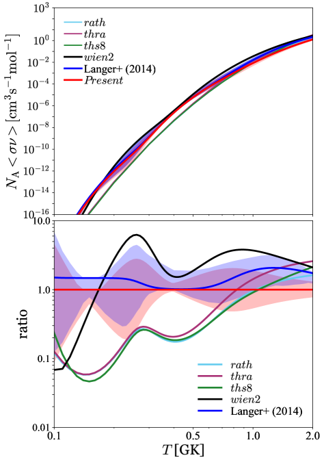
The comparison of the Present rate with Langer et al. rate and with other reaction rates compiled into JINA REACLIB v2.2 by Cyburt et al. (2010) is shown in Fig. 4. The Hauser-Feshbach statistical model rates, i.e., rath¹¹1Produced by Rauscher & Thielemann (2000) using Non-Smoker code with FRDM mass input (Möller et al., 1995)., thra²²2Ibid., with ETFSI-Q mass input (Pearson et al., 1996)., and ths8³³3Produced by T. Rauscher using Non-Smoker code as part of JINA REACLIB since the v1.0 release (Cyburt et al., 2010). are very close to one another from $0.1$ to $2.0$ GK, and they are lower than the Present rate up to an order of magnitude at temperature $T\lesssim 0.9$ GK. Due to the reduction of the contribution from the $1^{+}_{2}$ resonance state, the Present rate is up to a factor of two lower than Langer et al. rate from $0.8$ to $2$ GK covering the typical maximum temperature of GS 1826 $-$ 24 burster, and up to a factor of four lower than the wien2 rate (Forstner et al., 2001) recommended by JINA REACLIB v2.2, see the comparison in the respective ratio in the bottom panel of Fig. 4.

By taking into account the uncertainty of $S_{\mathrm{p}}$ (⁵⁸Zn), we estimate and list the uncertainty of Present ⁵⁷Cu(p, $\gamma$ )⁵⁸Zn reaction rate as upper and lower limits in Table 5. Both upper and lower limits are shown as red zone in Fig. 4, whereas the uncertainty of Langer et al. rate is indicated as blue zone. Even if the uncertainty due to the order of $1^{+}_{1}$ and $2^{+}_{3}$ states would have been removed, the uncertainty of $S_{\mathrm{p}}$ (⁵⁸Zn) propagated from the measured ⁵⁸Zn mass (Seth et al., 1986) is still dominant and persistent. Note that this is the first ⁵⁷Cu(p, $\gamma$ )⁵⁸Zn reaction rate constructed from important experimental information supplemented with the full $pf$ -shell space shell-model calculation that yields converged resonance energies, $\Gamma_{\gamma}$ , and spectroscopic factors; and the uncertainty is clearly identified, whereas the Hauser-Feshbach statistical model rates may include unknown systematic errors because of their limited capability in estimating level densities of nuclei near to the proton drip line.

4 Implication on multi-zone X-ray burst models

We explore the influence of the Present ⁵⁷Cu(p, $\gamma$ )⁵⁸Zn reaction rate on characterizing the XRB light curves of the GS 1826 $-$ 24 X-ray source (Makino et al., 1988; Tanaka et al., 1989) and burst ash composition after an episode of XRBs based on one-dimensional multi-zone hydrodynamic XRB models. The theoretical XRB models matched with the GS 1826 $-$ 24 clocked burster (Ubertini et al., 1999) are instantiated by the Kepler code (Weaver et al., 1978; Woosley et al., 2004; Heger et al., 2007) and were used by Heger et al. (2007) to perform the first quantitative comparison with the observed GS 1826 $-$ 24 light curve. Later, the GS 1826 $-$ 24 XRB models were used by Cyburt et al. (2016) and by Jacobs et al. (2018) to study the sensitivity of $(\alpha,\gamma)$ , ( $\alpha$ ,p), (p, $\gamma$ ), and (p, $\alpha$ ) nuclear reactions. The GS 1826 $-$ 24 XRB models are continuously updated and were recently used by Goodwin et al. (2019) and by Johnston et al. (2020) to study the high density properties of accreted envelopes of GS 1826 $-$ 24 clocked burster. The XRB models are fully self-consistent, which take into account of the correspondence between the evolution in astrophysical conditions and the feedback of nuclear energy generation in substrates of accreted envelope. Throughout an episode of outbursts, which may consist of a series of bursts with either an almost consistent or progressively increasing recurrence time, the models are capable to keep updating the evolution of chemical inertia and thermal configurations that drive the nucleosynthesis in the accreted envelope of an accreting neutron star.

The XRB models simulate a grid of Lagrangian zones (Weaver et al., 1978; Woosley et al., 2004; Heger et al., 2007), and each zone independently contains its own isotopic composition and thermal properties. We implement the time-dependent mixing length theory (Heger et al., 2000) to describe the convection transferring heat and nuclei between these Lagrangian zones. Kepler uses an adaptive thermonuclear reaction network that automatically includes or discards the respective reactions out of the more than 6000 isotopes provided by JINA REACLIB v2.2 (Cyburt et al., 2010).

We adopt the XRB model from Jacobs et al. (2018) to compare with the observed burst light curves of the GS 1826 $-$ 24 clocked burster. The model had been used by Jacobs et al. (2018) in a recent sensitivity study of nuclear reactions. To match the modeled light curve with the observed light curve and recurrence time, $\Delta t_{\mathrm{rec}}=5.14\pm 0.7$ h, of Epoch Jun 1998 of GS 1826 $-$ 24 burster, we adjust the accreted ¹H, ⁴He, and CNO metallicity fractions to $0.71$ , $0.2825$ , and $0.0075$ , respectively. The accretion rate is tuned to a factor of $0.122$ of the Eddington-limited accretion rate, $\dot{M}_{\mathrm{Edd}}$ . This adjusted XRB model with the associated nuclear reaction library (JINA REACLIB v2.2) characterizes the baseline model in this work. Note that the wien2 rate is the recommended ⁵⁷Cu(p, $\gamma$ )⁵⁸Zn reaction rate in JINA REACLIB v2.2. Other XRB models that adopt the same astrophysical configurations but implement the Present ⁵⁷Cu(p, $\gamma$ )⁵⁸Zn; or the corrected ⁵⁵Ni(p, $\gamma$ )⁵⁶Cu (Valverde et al., 2019); or the Present ⁵⁷Cu(p, $\gamma$ )⁵⁸Zn and Valverde et al. corrected ⁵⁵Ni(p, $\gamma$ )⁵⁶Cu; or Langer et al. ⁵⁷Cu(p, $\gamma$ )⁵⁸Zn, Valverde et al. corrected ⁵⁵Ni(p, $\gamma$ )⁵⁶Cu, and (Kahl et al., 2019) ⁵⁶Ni(p, $\gamma$ )⁵⁷Cu; or the Present ⁵⁷Cu(p, $\gamma$ )⁵⁸Zn, Valverde et al. corrected ⁵⁵Ni(p, $\gamma$ )⁵⁶Cu, and Kahl et al. ⁵⁶Ni(p, $\gamma$ )⁵⁷Cu reaction rates are denoted as Present^†, Present^‡, Present^♠, Present^♡, and Present^§ models, respectively. The Present^♡ and Present^§ models implement a factor of $0.120$ of $\dot{M}_{\mathrm{Edd}}$ for the accretion rate in order to obtain a modeled recurrence time close to the observation, proposing that either Present or Langer et al. ⁵⁷Cu(p, $\gamma$ )⁵⁸Zn reaction rate, which is lower than the wien2 rate, shortens the recurrence time by up to $5$ %.

We then simulate a series of 40 consecutive XRBs for baseline, Present^†, Present^‡, Present^♠, Present^♡, and Present^§ models; and only the last 30 bursts are summed up with respect to the time resolution and then averaged to yield a burst light-curve profile. The first 10 bursts simulated from each model are excluded because these bursts undergo a transition from a chemically fresh envelope with unstable burning to an enriched envelope with chemically burned-in burst ashes and stable burning. Throughout the transition, the enriched burst ashes are recycled in the succeeding burst heating which gradually stabilize the following bursts. The averaging procedure applied on the modeled light curves is similar to the method performed by Galloway et al. (2017) to produce an averaged light-curve profile from the observed data set of Epoch Jun 1998. The epoch was recorded by the Rossi X-ray Timing Explorer (RXTE) Proportional Counter Array (Galloway et al., 2004, 2008, 2020) and were compiled into the Multi-Instrument Burst Archive⁴⁴4https://burst.sci.monash.edu/minbar/ by Galloway et al. (2020).

The yielded burst luminosity, $L_{\mathrm{x}}$ , from each model is transformed and related to the observed flux, $F_{\mathrm{x}}$ , via the relation (Johnston et al., 2020),

\displaystyle F_{\mathrm{x}}=

\displaystyle\frac{L_{\mathrm{x}}}{4\pi d^{2}\xi_{\mathrm{b}}(1+z)^{2}}\,,

(12)

where $d$ is the distance; $\xi_{\mathrm{b}}$ takes into account of the possible deviation of the observed flux from an isotropic burster luminosity due to the scattering and blocking of the emitted electromagnetic wave by the accretion disc (Fujimoto et al., 1988; He et al., 2016); and the redshift, $z$ , re-scales the light curve when transforming into an observer’s frame. The $d$ and $\xi_{\mathrm{b}}$ are combined to form the modified distance $d\sqrt{\xi_{\mathrm{b}}}$ by assuming that the anisotropy factors of burst and persistent emissions are degenerate with distance. We include the entire burst timespan of an averaged observational data to fit our modeled burst light curves of each model to the observed light curve. The best-fit $d\sqrt{\xi_{\mathrm{b}}}$ and $(1+z)$ factors of the baseline, Present^†, Present^‡, Present^♠, Present^♡, and Present^§ modeled light curves to the averaged-observed light curve and recurrence time of Epoch Jun 1998 are $7.28$ kpc and $1.29$ , $7.32$ kpc and $1.29$ , $7.32$ kpc and $1.29$ , $7.32$ kpc and $1.28$ , $7.30$ kpc and $1.29$ , $7.62$ kpc and $1.29$ , respectively. Using these redshift factors, we obtain a set of modeled recurrence times which are close to the observation. The recurrence times of baseline, Present^†, Present^‡, Present^♠, Present^♡, and Present^§, are $4.85$ h, $4.91$ h, $4.91$ h, $4.88$ h, $4.96$ h, and $4.95$ h, respectively. Though further reducing the accretion rate for each model improves the matching between modeled and observed recurrence time, all modeled burst light curves remain similar. For instance, the recurrence time of the Present^§ model $\Delta t_{\mathrm{rec}}=4.95$ h is produced with defining accretion rate as $0.120$ $\dot{M}_{\mathrm{Edd}}$ and the produced burst light curve is similar to other modeled light curves in the present work.

Figure 6: The nucleosynthesis and evolution of envelope corresponds to the moment just before the onset of the 39^th burst for baseline (Top Left Panel), of the 42^nd for Present^♡ (Top Right Panel), and of the 41^st burst for Present^§ (Bottom Left Panel) scenarios. The averaged abundances of synthesized nuclei are represented by color tones referring to the right color scale in the nuclear chart of each panel. The black squares are stable nuclei. The top left insets in each panel magnify the regions related to the NiCu and ZnGa cycles. Pointing upward arrows indicate the (p,

\gamma

) reactions, whereas pointing downward arrows show the photodisintegration (

\gamma

,p) reactions. Slanting arrows from left to right depict (

\beta^{+}\nu

) decays and long slanting arrows from right to left represent (p,

\alpha

) reactions. These arrows are merely used to guide the eyes. The bottom right insets in each panel present the corresponding temperature (black dotted line) and density (black dashed line) of each mass zone, referring to right the

y

-axis, and the abundances of synthesized nuclei, referring to the left

y

-axis, in the accreted envelope regime where nuclei heavier than CNO isotopes are densely synthesized. The abundances of H and He are represented by black and red solid lines, respectively. Bottom Right Panel: The comparisons of abundances of ⁵⁵Ni, ⁵⁶Cu, ⁵⁷Zn, ⁵⁶Ni, ⁵⁷Cu, and ⁵⁸Zn of baseline, Present^♡, and Present^§ at the respective time snapshot. These abundances are plotted with respect to the mass coordinate of the baseline accreted envelope regime.

Figure 7: The nucleosynthesis and evolution of envelope corresponds to the moment at the immediate vicinity of the burst peak for baseline (Top Left Panel), Present^♡ (Top Right Panel), and Present^§ (Bottom Left Panel) scenarios. See Fig. 6 for further description.

Figure 8: The nucleosynthesis and evolution of envelope corresponds to the moment of around 14 s after the burst peak for baseline (Top Left Panel), Present^♡ (Top Right Panel), and Present^§ (Bottom Left Panel) scenarios. See Fig. 6 for further description.

Figure 9: The nucleosynthesis and evolution of envelope corresponds to the moment of around 180 s after the burst peak for baseline (Top Left Panel), Present^♡ (Top Right Panel), and Present^§ (Bottom Left Panel) scenarios. See Fig. 6 for further description.

The top panel of Fig. 5 illustrates the comparison between the best-fit modeled and observed XRB light curves. The evolution time of light curve is relative to the burst-peak time, $t=0$ s. The overall averaged flux deviations between the observed epoch and each of these theoretical models, baseline, Present^†, Present^‡, Present^♠, Present^♡, and Present^§, in units of $10^{-9}\mathrm{erg~{}cm}^{-2}\mathrm{s}^{-1}$ are $1.154$ , $1.170$ , $1.172$ , $1.133$ , $1.181$ , and $1.147$ , respectively. The deviations between the Present^§ (and baseline) and observed light curve throughout the whole timespan of the observed light curve are displayed in the bottom panel of Fig. 5.

The observed burst peak is thought to be located in the time regime $t=-2.5$ s – 2.5 s (top left inset in Fig. 5), and at the vicinity of the modeled light-curve peaks of baseline, Present^†, Present^‡, Present^♠, Present^♡, and Present^§. The modeled light curves of baseline, Present^†, Present^‡, Present^♠, Present^♡, and Present^§ at the near-burst-peak region $t=-4.5$ s – $5.5$ s are almost indiscernible.

All modeled light curves are less enhanced than the observed light curve at $t=8$ s – $80$ s, and the decrement is even augmented at around $t=13$ s and $40$ s, increasing the deviation between the modeled and observed light curves (bottom panel in Fig. 5). From the time regime at $t=78$ s onward until the burst tail end, all modeled burst light curves are enhanced. Overall, all modeled light-curve profiles are similar and note that the observed burst tail is reproduced from $t=78$ s onward until the burst tail end.

To investigate the microphysics behind the difference between both modeled burst light curves of the baseline and Present^§ models, we consider the 39^th, the 42^nd, and the 41^st burst for the baseline, Present^♡, and Present^§ models, respectively. These bursts resemble the respective averaged light curve profile presented in Fig. 5. The reference time of accreted envelope and nucleosynthesis in the following discussion is also relative to the burst-peak time, $t=0$ s.

The moment before and during the onset.

After the preceding burst, the synthesized proton-rich nuclei in the accreted envelope go through $\beta^{+}$ decays and enrich the region around stable nuclei with long half-lives, e.g., ⁶⁰Ni, ⁶⁴Zn, ⁶⁸Ge, and ⁷⁸Se, which are the remnants of waiting points. When the accreted envelope evolves to the moment just before the onset of the succeeding XRB, due to the continuing nuclear reactions that occur in unburned hydrogen above the base of the accreted envelope, the temperature of the envelope increases up to a maximum value of about $0.93$ GK at the moment $t=-10$ s for the baseline, Present^♡, and Present^§ scenarios, see Fig. 6. At the moment just before the onset, some nuclei have already been synthesized and stored in the NiCu cycles, i.e., the NiCu I and II cycles (Van Wormer et al., 1994), and the sub-NiCu II cycle (Fig. 1), see the top left and bottom right insets of the top left, bottom left, and top right panels of Fig. 6. Among the isotopes in the NiCu cycles, the highly synthesized nuclei having mass fractions of more than 2 $\times 10^{-4}$ are ⁵⁹Zn, ⁵⁸Zn, ⁵⁷Zn, ⁵⁸Ni, ⁵⁹Cu, ⁵⁸Cu, ⁵⁷Cu, ⁶⁰Cu isotopes, and the ⁵⁶Ni and ⁶⁰Zn waiting points, whereas the ⁵⁶Co and ⁶⁰Cu isotopes having analogous mass-fraction distributions in the envelope are converted to ⁵⁷Ni and ⁶¹Zn, respectively (the lower right insets in the top left, bottom left, and top right panels of Fig. 6).

We find that although the reaction flow induced by the ⁵⁵Ni(p, $\gamma$ )⁵⁶Cu(p, $\gamma$ )⁵⁷Zn branch noticeably bypasses the ⁵⁶Ni waiting point and enriches ⁵⁷Zn for the baseline, Present^♡, and Present^§ scenarios, it eventually has to go through the ⁵⁷Zn( $\beta^{+}\nu$ )⁵⁷Cu(p, $\gamma$ )⁵⁸Zn branch and combines with the NiCu cycles and then breaks out from the NiCu cycles to the ZnGa cycles, see the upper left insets in the top left, bottom left, and top right panels of Fig. 6. Due to the rather weak ⁵⁷Zn(p, $\gamma$ )⁵⁸Ga reaction, the ⁵⁵Ni(p, $\gamma$ )⁵⁶Cu(p, $\gamma$ )⁵⁷Zn reactions and the subsequent ⁵⁷Zn( $\beta^{+}\nu$ )⁵⁷Cu(p, $\gamma$ )⁵⁸Zn branch redirect an appreciable amount material away from the ⁵⁶Ni waiting point, but the redirecting branch does not store material. Moreover, the newly corrected ⁵⁵Ni(p, $\gamma$ )⁵⁶Cu reaction rate is lower than the one recommended in JINA REACLIB v2.2 (Fig. 2), causing less enrichment of ⁵⁷Zn in the Present^♡ and Present^§ scenarios (bottom right panel of Fig. 6). This explains why neither the newly corrected nor the recommended ⁵⁵Ni(p, $\gamma$ )⁵⁶Cu reaction rate exhibiting significant influence on the light curve of GS 1826 $-$ 24 burster and abundances of synthesized heavier nuclei. Also, the corrected ⁵⁵Ni(p, $\gamma$ )⁵⁶Cu reaction rate is not as influential as claimed by Valverde et al. (2018, 2019). Note that the one-zone models used by Valverde et al. (2018, 2019) do not reproduce any burst light curves that are matched with observations. We remark that the baseline model that uses the recommended ⁵⁵Ni(p, $\gamma$ )⁵⁶Cu reaction rate in JINA REACLIB v2.2 has already manifested the possibility of the bypassing reaction flow of the ⁵⁶Ni waiting point without replacing the recommended rate by Valverde et al. (2019) corrected rate because the recommended ⁵⁵Ni(p, $\gamma$ )⁵⁶Cu reaction rate is stronger than the Valverde et al. corrected reaction rate, see Fig. 2.

At this moment, more than $60$ % of mass zones in the accreted envelope, where nuclei heavier than CNO isotopes are densely synthesized, is with temperature above $0.8$ GK. The Present ⁵⁷Cu(p, $\gamma$ )⁵⁸Zn reaction rate is up to a factor of $2$ lower than Langer et al. rate from $0.8$ GK to $2$ GK due to the reduction of the domination of $1^{+}_{2}$ resonance state (bottom panel of Fig. 4), reducing the transmutation rate of ⁵⁷Cu to ⁵⁸Zn. This situation impedes the ⁵⁶Ni(p, $\gamma$ )⁵⁷Cu(p, $\gamma$ )⁵⁸Zn reaction flow while enhances the reaction flow by-passing the important ⁵⁶Ni waiting point, causing a higher production of ⁵⁵Ni in the Present^§ scenario (bottom right panel of Fig. 6). Meanwhile, Valverde et al. corrected ⁵⁵Ni(p, $\gamma$ )⁵⁶Cu reaction rate implemented in the Present^§ scenario reduces the production of ⁵⁷Zn, and induces the reaction flow to ⁵⁷Cu. These reaction flows are regulated with new reaction rates and then produce a rather similar ⁵⁸Zn abundance in the baseline and Present^§ scenarios that are about a factor of $1.2$ higher than the ⁵⁸Zn abundance in the Present^♡.

Note that the productions of ⁵⁵Ni, ⁵⁶Cu, ⁵⁷Zn, ⁵⁶Ni, ⁵⁷Cu, and ⁵⁸Zn based on the Present^♡ and Present^§ are discernible due to the correlated influence among the Present (or Langer et al. (2014)) ⁵⁷Cu(p, $\gamma$ )⁵⁸Zn, Valverde et al. (2019) corrected ⁵⁵Ni(p, $\gamma$ )⁵⁶Cu, and Kahl et al. (2019) ⁵⁶Ni(p, $\gamma$ )⁵⁷Cu reaction rates. The continuous impact from the correlated influence among these reactions and ⁵⁹Cu(p, $\alpha$ )⁵⁶Ni that cycles the reaction flow back to the reaction series in the NiCu cycles since the onset later influences the burst ash composition at the burst tail end.

The mass fraction of ⁵⁷Cu in the baseline is lower than the one in the Present^♡ and Present^§ scenarios because the newly updated ⁵⁶Ni(p, $\gamma$ )⁵⁷Cu by Kahl et al. (2019) implemented in Present^♡ and Present^§ is about up to a factor of 9 higher than the recommended ⁵⁶Ni(p, $\gamma$ )⁵⁷Cu rate from JINA REACLIB v2.2 used in baseline at temperature region around 1 GK. Nevertheless, the mass fraction of ⁵⁸Zn in the baseline is about a factor of 1.2 higher than the one in the Present^§ scenario. This reflects a stronger flow of ⁵⁷Cu(p, $\gamma$ )⁵⁸Zn in the baseline than in the Present^§ scenario. Such stronger flow is because the recommended wien2 ⁵⁷Cu(p, $\gamma$ )⁵⁸Zn reaction rate from JINA REACLIB v2.2 used in baseline is about up to a factor of 4 higher than the Present ⁵⁷Cu(p, $\gamma$ )⁵⁸Zn reaction rates at temperature region around 1 GK. Meanwhile, the induced ⁵⁷Zn( $\beta^{+}\nu$ )⁵⁷Cu flow from the reaction flow by-passing the important ⁵⁶Ni waiting point stacks up the abundance of ⁵⁷Cu in the Present^§ scenario. Hence, a strong flow of the ⁵⁶Ni(p, $\gamma$ )⁵⁷Cu coupled with a weak flow of the ⁵⁷Cu(p, $\gamma$ )⁵⁸Zn in the Present^§ scenario and the stacked up ⁵⁷Cu eventually yield a set of almost similar mass fractions of ⁵⁸Zn along the mass zones in the accreted envelope during the onset for both baseline and Present^§ scenarios. On the other hand, the synthesized nuclei heavier than ⁶⁸Se for the baseline is almost as extensive as the Present^§ scenario, see the nuclear chart in Fig. 6. This indicates the reaction flow is regulated at the ⁶⁰Zn waiting point by the ⁵⁹Cu(p, $\alpha$ )⁵⁶Ni reaction that competes with the ⁵⁹Cu(p, $\gamma$ )⁶⁰Zn reaction. Furthermore, after the reaction flow breaks out from the NiCu cycles through the ⁵⁹Cu(p, $\gamma$ )⁶⁰Zn(p, $\gamma$ )⁶¹Ga branch to the ZnGa cycles (Van Wormer et al., 1994), it is stored in the ZnGa cycles before surging through the nuclei heavier than ⁶⁸Se. We find that the GeAs cycle that involves two-proton sequential capture of ⁶⁴Ge consisting of ⁶⁴Ge(p, $\gamma$ )⁶⁵As(p, $\gamma$ )⁶⁶Se reactions could weakly exist in the mid of onset until the moment after burst peak (Lam et al., 2022a), see the nucleosynthesis charts in Figs. 6, 7, and 8. A new ⁶⁵As(p, $\gamma$ )⁶⁶Se reaction rate based on a more precise ⁶⁶Se mass is desired to constrain the transient period, nonetheless, the fact that the transient existence of the weak GeAs cycle is not ruled out for the GS 1826 $-$ 24 burster.

The ZnGa cycles have been recently investigated by Lam et al. (2022b) using the same GS 1826 $-$ 24 clocked burster model as is used in this work and the full $pf$ -model space shell model calculation. They found that the GeAs cycle that follows the ZnGa cycles only weakly exists for a brief period, which could last until $t=21.4$ s – $58.6$ s after the burst peak (Lam et al., 2022a). This causes some reactions relevant to the ZnGa cycles becomes decisive in controlling the reaction flow reaching nuclei heavier than Ge and Se isotopes where the extensive H-burning via (p, $\gamma$ ) reactions occur. These influential reactions are ⁵⁹Cu(p, $\gamma$ ) and ⁶¹Ga(p, $\gamma$ ), which were identified and marked by Cyburt et al. (2016) as the top four most sensitive reactions on clocked burst light curve. Lam et al. (2022b) found that the ⁵⁹Cu(p, $\gamma$ ) and ⁶¹Ga(p, $\gamma$ ) reactions characterize the burst light curve of the GS 1826 $-$ 24 clocked burster at $t\approx 8$ s – $30$ s after the burst peak and the burst tail end. Preliminary results of the investigation of the ZnGa cycles were presented in the Supplemental Material of Hu et al. (2021) prior to Lam et al. (2022b) publication.

We notice that the balance between the ⁵⁶Ni(p, $\gamma$ )⁵⁷Cu and ⁵⁷Cu(p, $\gamma$ )⁵⁸Zn reactions also redistributes the reaction flow to the NiCu II cycle and then the reaction flow eventually joins with the NiCu I cycle and branches out to the ZnGa cycles at the ⁶⁰Zn waiting point or follows the ⁶⁰Cu(p, $\gamma$ )⁶¹Zn(p, $\gamma$ )⁶²Ga reactions branches out to the ZnGa II cycle. Then, the joint reaction flow surges through the proton-rich region heavier than ⁶⁴Ge where (p, $\gamma$ ) reactions actively burn hydrogen and intensify the rise of burst light curve from $t=-10$ s up to $t=0$ s (burst peak).

The moment at the immediate vicinity of burst peak.

As the redistributing and reassembling of reaction flow from the moment of onset until the burst peak regulate a rather similar feature of abundances in the NiCu cycles (the lower right insets in the top left, bottom left, and top right panels of Fig. 7), and the maximum envelope temperature of the baseline, Present^♡, and Present^§ scenarios are rather similar. These outcomes cause burst peaks of the baseline, Present^♡, and Present^§ scenarios almost close to each other, see the left inset in the upper panel of Fig. 5 and the maximum envelope temperatures in Fig. 7.

The moment after the burst peak.

At $t\!\approx\!14$ s and $T\approx\!1.06$ GK (maximum envelope temperature), the redistributing of reaction flow since the moment of onset mentioned above slightly keeps the reaction flow in NiCu cycles for somehow longer time and slightly delays the reaction flow from passing through the waiting point ⁶⁰Zn in the Present^§ scenario. The small delay allows the reaction flow to leak out from the NiCu cycles at later time and to burn hydrogen along the way reaching isotopes heavier than ⁶⁸Se via (p, $\gamma$ ) reactions, and this situation mildly deviates the burst light curve of Present^§ from the light curves of baseline and Present^♡.

The moment at the burst tail end.

The observed burst tail end of Epoch Jun 1998 of GS 1826 $-$ 24 burster is closely reproduced by the baseline, Present^♡, and Present^§ models, meaning that the H-burning in these models recesses accordingly to produce a set modeled light curves in good agreement with observation. At $t=85$ s, the light curves of baseline and Present^♡ deviate from the light curve of Present^§ about $0.3\times 10^{-9}\mathrm{erg~{}cm}^{-2}\mathrm{s}^{-1}$ . Based on the analysis of the influence of ⁵⁷Cu(p, $\gamma$ )⁵⁸Zn reaction rate, we anticipate that if the actual energies of $1^{+}_{2}$ and $2^{+}_{5}$ resonance states are even higher than the presently estimated ones using the IMME formalism, the contributions of these two resonance states to the total rate are exponentially reduced, and the $2^{+}_{4}$ resonance state becomes the only dominant resonance at $T=1$ GK – $2$ GK for the ⁵⁷Cu(p, $\gamma$ )⁵⁸Zn reaction rate, and thus the modeled burst light curve is more diminished at the burst peak and at $t=8$ s – $32$ s, whereas at $t=65$ s – $150$ s, the Present^§ light curve is more enhanced compared to the baseline scenario.

From $t\!\!\approx\!\!14$ s onward until $t\!\approx\!180$ s, the regulation of NiCu cycles gradually deviates for the production of ⁵⁸Zn due to the cumulated effect from the correlated influence among the latest ⁵⁶Ni(p, $\gamma$ )⁵⁷Cu, ⁵⁷Cu(p, $\gamma$ )⁵⁸Zn, and ⁵⁵Ni(p, $\gamma$ )⁵⁶Cu reaction rates, despite of the suppression induced by the ⁵⁹Cu(p, $\alpha$ )⁵⁶Ni reaction, see the bottom right panel in Fig. 9. Although the lower limit of Langer et al. (2014) rate at $0.23$ GK $\lesssim T\lesssim 0.82$ GK is used for the Present^♡ model, the Present^♡ model still produces a set of ⁵⁵Ni, ⁵⁶Cu, and ⁵⁷Zn abundances lower than the ones of baseline and Present^§ models. Also, both baseline and Present^§ models produce similar ⁵⁵Ni, ⁵⁶Cu, and ⁵⁷Zn abundances. This indicates the cumulated impact that is generated from the difference of a factor of $2$ in temperature regime $T=0.8$ – $2$ GK between the Present and Langer et al. ⁵⁷Cu(p, $\gamma$ )⁵⁸Zn reaction rates. Meanwhile, the correlated influence on the syntheses of nuclei in the NiCu cycles is also manifested due to the Present ⁵⁷Cu(p, $\gamma$ )⁵⁸Zn, ⁵⁹Cu(p, $\alpha$ )⁵⁶Ni, Kahl et al. ⁵⁶Ni(p, $\gamma$ )⁵⁷Cu, and Valverde et al. ⁵⁵Ni(p, $\gamma$ )⁵⁶Cu reaction rates since the onset at $t=-10$ s.

The compositions of burst ashes generated by these three models are presented in Fig. 10. The cumulated impact from the regulated NiCu I, II, and sub-II cycles based on the Present and Langer et al. ⁵⁷Cu(p, $\gamma$ )⁵⁸Zn reaction rates manifests on the abundances of burst ashes. Using the Present ⁵⁷Cu(p, $\gamma$ )⁵⁸Zn reaction rate, the production of ¹²C is reduced to a factor of $0.2$ , and thus the remnants from the hot CNO cycle, e.g., nuclei $A=17$ and $18$ are affected up to about a factor of $0.5$ and $2.5$ , respectively. The abundances of the daughters of SiP, SCl, and ArK cycles are reduced (increased) up to a factor of $0.7$ ( $1.2$ ). The total abundance of ⁵⁶Ni and its remnant is increased up to a factor of $1.2$ due to the correlated influence between the new ⁵⁶Ni(p, $\gamma$ )⁵⁷Cu, ⁵⁷Cu(p, $\gamma$ )⁵⁸Zn, and ⁵⁵Ni(p, $\gamma$ )⁵⁶Cu reaction rates. Meanwhile, the abundances of nuclei $A=64$ – $104$ produced by Present^§ are closer to baseline than the ones produced by Present^♡. Furthermore, the abundances of nuclei $A=105$ – $140$ are decreased up to a factor of 0.2 (red dots in the bottom panel of Fig. 10). Note that, the Present ⁵⁷Cu(p, $\gamma$ )⁵⁸Zn reaction rate produces a different set of burst ash composition deviating from the one generated by Langer et al. ⁵⁷Cu(p, $\gamma$ )⁵⁸Zn reaction rate, especially the burst ash composition of $sd$ -shell nuclei from $A=20$ – $34$ . Due to Langer et al. ⁵⁷Cu(p, $\gamma$ )⁵⁸Zn reaction rate, the abundances of nuclei $A=65$ – $84$ are reduced up to a factor of $0.9$ and the abundances of nuclei $A=100$ – $134$ are somehow closer to baseline than the ones generated from the Present ⁵⁷Cu(p, $\gamma$ )⁵⁸Zn reaction rate.

The noticeable difference in the burst ash compositions from the Present and from Langer et al. ⁵⁷Cu(p, $\gamma$ )⁵⁸Zn reaction rates exhibits the sensitivity of the ⁵⁷Cu(p, $\gamma$ )⁵⁸Zn reaction in influencing the burst ash composition that eventually affects the composition of the neutron-star crust. Therefore, the presently more constrained ⁵⁷Cu(p, $\gamma$ )⁵⁸Zn coupled with the latest ⁵⁶Ni(p, $\gamma$ )⁵⁷Cu and ⁵⁵Ni(p, $\gamma$ )⁵⁶Cu reaction rates constricts the burst ash composition which is the initial input for studying superburst (Gupta et al., 2007).

5 Summary and conclusion

A theoretical study of ⁵⁷Cu(p, $\gamma$ )⁵⁸Zn reaction rate is performed based on the large-scale shell-model calculations in the full pf-model space using GXPF1a and its charge-dependent version, cdGX1A, interactions. We present a detailed analysis of the energy spectrum of ⁵⁸Zn on the basis of the IMME concept with the aim to determine the order of $1^{+}_{1}$ and $2^{+}_{3}$ states of ⁵⁸Zn that are dominant in the ⁵⁷Cu(p, $\gamma$ )⁵⁸Zn reaction rate at $T=0.3$ – $0.8$ GK. As no firm assignment can be done due to the lack of experimental information on ⁵⁸Cu spectrum, we test an alternative assignment to the previously adopted one. We have also estimated the energy of $1^{+}_{2}$ state of ⁵⁸Zn based on the presently available candidate for isobaric analogue states of ⁵⁸Cu and ⁵⁸Ni, which were experimentally determined, and the theoretical IMME $c$ coefficient. We estimate the $1^{+}_{2}$ state of ⁵⁸Zn to be higher than the one predicted by the isospin conserving interaction pf-shell interaction, GXPF1a. The dominance of the $1^{+}_{2}$ state in the ⁵⁷Cu(p, $\gamma$ )⁵⁸Zn reaction rate at $T=0.8$ – $2$ GK is exponentially reduced. Throughout the course of a clocked burst, more than $60$ % of the mass zones in the accreted envelope is heated to $T=0.8$ – $1.6$ GK. The clocked XRBs of the GS 1826 $-$ 24 burster is more sensitive to the ⁵⁷Cu(p, $\gamma$ )⁵⁸Zn reaction rate at the temperature range $0.8\lesssim T$ (GK) $\lesssim 1.6$ GK. Thus, the resonance energy of the dominant $1^{+}_{2}$ state determining the ⁵⁷Cu(p, $\gamma$ )⁵⁸Zn reaction rate at $T=0.8$ – $1.6$ GK is important in influencing the extent of synthesized nuclei during clocked bursts of GS 1826 $-$ 24 burster.

Using the newly deduced ⁵⁷Cu(p, $\gamma$ )⁵⁸Zn, the newly corrected ⁵⁵Ni(p, $\gamma$ )⁵⁶Cu, and the updated ⁵⁶Ni(p, $\gamma$ )⁵⁷Cu reaction rates, we find that five combinations of these three reactions yield a set of light-curve profiles similar to the one generated by the baseline model based on the Forstner et al. (2001) and Fisker et al. (2001) reaction rates which are labeled as wien2 and nfis, respectively, in JINA REACLIB v2.2. Nevertheless, the correlated influence on the nucleosyntheses exhibits that the ⁵⁷Cu(p, $\gamma$ )⁵⁸Zn reaction is critical in characterizing the burst ash composition. Constraining the ⁵⁷Cu(p, $\gamma$ )⁵⁸Zn reaction rate lower than a factor of $5$ difference in between the Present and wien2 ⁵⁷Cu(p, $\gamma$ )⁵⁸Zn reaction rates and than a factor of $2$ difference in between the Present and Langer et al. ⁵⁷Cu(p, $\gamma$ )⁵⁸Zn reaction rates at the temperature regime relevant for XRBs is important for us to have a more constrained initial neutron-star crust composition. We remark that the observed burst tail end of Epoch Jun 1998 of GS 1826 $-$ 24 burster is closely reproduced by all models of the present work with the slightly adjusted astrophysical parameters.

Furthermore, we find that the redistributing and reassembling of reaction flows in the NiCu cycles also diminish the impact of ⁵⁵Ni(p, $\gamma$ )⁵⁶Cu reaction though this by-passing reaction partially diverts material from the ⁵⁶Ni waiting point, the reaction flow eventually joins with the NiCu cycles and leaks out to the ZnGa cycles. Indeed, as indicated by the one-dimensional multi-zone hydrodynamic XRB model matching with the GS 1826 $-$ 24 clocked burster, implementing the nfis ⁵⁵Ni(p, $\gamma$ )⁵⁶Cu reaction rate has already manifested the bypassing reaction flow of the ⁵⁶Ni waiting point without the implementation of Valverde et al. (2019) ⁵⁵Ni(p, $\gamma$ )⁵⁶Cu reaction rate.

In addition, we notice that the weak GeAs cycle involving the two-proton sequential capture on ⁶⁴Ge, following the ⁶⁴Ge(p, $\gamma$ )⁶⁵As(p, $\gamma$ )⁶⁶Se branch may exist shortly around the mid of onset until after the burst peak. The period of this transient existence may depend on the precise determination of the $S_{\mathrm{p}}$ (⁶⁶Se) value. The Present ⁵⁷Cu(p, $\gamma$ )⁵⁸Zn reaction rate, which is more constrained than Langer et al. (2014) reaction rate, was used by Lam et al. (2022a) to study the weak GeAs cycles, and was also recently used by Hu et al. (2021) to study the prevail influence of the newly deduced ²²Mg( $\alpha$ ,p)²⁵Al.

We are very grateful to N. Shimizu for suggestions in tuning the KShell code at the PHYS_T3 (Institute of Physics) and QDR4 clusters (Academia Sinica Grid-computing Centre) of Academia Sinica, Taiwan, to D. Kahl for checking and implementing the newly updated ⁵⁶Ni(p, $\gamma$ )⁵⁷Cu reaction rate, to B. Blank for implementing the IMME framework, to M. Smith for using the Computational Infrastructure for Nuclear Astrophysics, to B. A. Brown for using the NuShellX@MSU code, and to J. J. He for fruitful discussion. This work was financially supported by the Strategic Priority Research Program of Chinese Academy of Sciences (CAS, Grant Nos. XDB34000000 and XDB34020204) and National Natural Science Foundation of China (No. 11775277). We are appreciative of the computing resource provided by the Institute of Physics (PHYS_T3 cluster) and the ASGC (Academia Sinica Grid-computing Center) Distributed Cloud resources (QDR4 cluster) of Academia Sinica, Taiwan. Part of the numerical calculations were performed at the Gansu Advanced Computing Center. YHL gratefully acknowledges the financial supports from the Chinese Academy of Sciences President’s International Fellowship Initiative (No. 2019FYM0002) and appreciates the laptop (Dell M4800) partially sponsored by Pin-Kok Lam and Fong-Har Tang during the pandemic of Covid-19. A.H. is supported by the Australian Research Council Centre of Excellence for Gravitational Wave Discovery (OzGrav, No. CE170100004) and for All Sky Astrophysics in 3 Dimensions (ASTRO 3D, No. CE170100013). N.A.S. is supported by the IN2P3/CNRS, France, Master Project – “Exotic nuclei, fundamental interactions and astrophysics”.

References

Angulo et al. (1999) Angulo, C., Arnould, M., Rayet, M., et al. 1999, Nucl. Phys. A, 656, 3
Audi et al. (2016) Audi, G., Kondev, F. G., Wang, M., et al. 2017, \chphc, 41, 030001
Brown (2014) Brown, B. A. (WSPOT code), http://www.nscl.msu.edu/ $\sim$ brown/reaction-codes/home.html
Brown & Rae (2014) Brown, B. A. & Rae, W. D. M. 2014, \nds, 120, 115
Brussaard & Glaudemans (1977) Brussaard, P. J., Glaudemans, P. W. M. 1977, Shell model Applications in Nuclear Spectroscopy (North-Holland, Amsterdam)
Cyburt et al. (2010) Cyburt, R. H., Amthor, A. M., Ferguson, R., et al. 2010, ApJS, 189, 240
Cyburt et al. (2016) Cyburt, R. H., Amthor, A. M., Heger, A., et al. 2016, ApJ, 830, 55
Fisker et al. (2001) Fisker, J. L., Barnard, V., Görres, J., et al. 2001, \adndt, 79, 241
Forstner et al. (2001) Forstner, O., Herndl, H., Oberhummer, H., et al. 2001, Phys. Rev. C, 64, 045801
Fowler et al. (1964) Fowler, W. A. & Hoyle, F. 1964, ApJS, 9, 201
Fowler et al. (1967) Fowler, W. A., Caughlan, G. R., Zimmerman, B. A. 1967, ARA&A, 5, 525
Fu et al. (2020) Fu, C. Y., Zhang, Y. H., Wang, M., et al. 2020, Phys. Rev. C, 102, 054311
Fujimoto et al. (1988) Fujimoto, M. Y. 1988, ApJ, 324, 995
Fujita et al. (2002) Fujita, Y., Fujita, H., Adachi, T., et al. 2002, \epja, 13, 411
Fujita et al. (2007) Fujita, H., Fujita, Y., Adachi, T., et al. 2007, Phys. Rev. C, 75, 034310
Galloway et al. (2004) Galloway, D. K., Cumming, A., Kuulkers, E., et al. 2004, ApJ, 601, 466
Galloway et al. (2008) Galloway, D. K., Muno, M. P., Hartman, J. M., et al. 2008, ApJS, 179, 360
Galloway et al. (2017) Galloway, D. K., Goodwin, A. J., Keek, L. 2017, PASA, 34, e019
Galloway et al. (2020) Galloway, D. K., in’ t Zand, J. J. M., et al. 2020, ApJS, 249, 32
Goodwin et al. (2019) Goodwin, A. J., Heger, A., Galloway, D. K. 2019, ApJ, 870, 64
Gupta et al. (2007) Gupta, S., Brown, E. F., Schatz, H., et al. 2007, ApJ, 662, 1188
He et al. (2016) He, C.-C. & Keek, L. 2016, ApJ, 819, 47
Heger et al. (2000) Heger, A., Langer, N., Woosley, S. E. 2000, ApJ, 528, 368
Heger et al. (2007) Heger, A., Cumming, A., Galloway, D. K., et al. 2007, ApJ, 671, L141
Herndl et al. (1995) Herndl, H., Görres, J., Wiescher, M., et al. 1995, Phys. Rev. C, 52, 1078
Honkanen et al. (1981) Honkanen, J., Kortelahti, M., Eskola, K., et al. 1981, Nucl. Phys. A, 366, 109
Honma et al. (2004) Honma, M., Otsuka, T., Brown, B. A., et al. 2004, Phys. Rev. C, 69, 034335
Honma et al. (2005) Honma, M., Otsuka, T., Brown, B. A., et al. 2005, \epja, 25(S01), 499
Horoi et al. (2007) Horoi, M., Stoica, S., Brown, B. A. 2007, Phys. Rev. C, 75, 034303
Hu et al. (2021) Hu, J., Yamaguchi, H., Lam, Y. H., et al. 2021, Phys. Rev. Lett., 127, 172701
Iliadis (2007) Iliadis, C. 2007, Nuclear Physics of Stars (Wiley, Weinheim)
Jacobs et al. (2018) Jacobs, A. M., Heger, A., et al. 2018, Burst Environment, Reactions and Numerical Modelling Workshop (BERN18), 11 – 15 Jun, Monash Prato Centre, Tuscany, Italy.
Johansson et al. (2009) Johansson, E. K., Rudolph, D., Ragnarsson, I., et al. 2009, Phys. Rev. C, 80, 014321
Johnston et al. (2020) Johnston, Z., Heger, A., Galloway, D. K. 2020, MNRAS, 494, 4576
Jongsma et al. (1972) Jongsma, H., Silva, A. D., Bron, J., et al. 1972, Nucl. Phys. A, 179, 554
Joss (1977) Joss, P. C. 1977, Nature, 270, 310
Joss (1978) Joss, P. C. 1978, ApJ, 225, L123
Kahl et al. (2019) Kahl, D., Woods, P. J., Poxon-Pearson, T., et al. 2019, \plb, 797, 134803
Keek & Heger (2011) Keek, L. and Heger, A. 2011, ApJ, 743, 189
Lam et al. (2013a) Lam, Y. H., Smirnova, N. A., Caurier, E. 2013, Phys. Rev. C, 87, 054304
Lam et al. (2013b) Lam, Y. H., Blank, B., Smirnova, N. A., et al. 2013, \adndt, 99, 680
Lam et al. (2016) Lam, Y. H., He, J. J., Parikh, A., et al. 2016, ApJ, 818, 78
Lam et al. (2022a) Lam, Y. H., Liu, Z. X., Heger, A., et al., accepted by The Astrophysical Journal on 10 Jan 2022, arXiv:2110.13676
Lam et al. (2022b) Lam, Y. H., Lu, N., Heger, A., et al., 2022, (to be published).
Langer et al. (2014) Langer, C., Montes, F., Aprahamian, A., et al. 2014, Phys. Rev. Lett., 113, 032502
Ma et al. (2019) Ma, S. -B., Zhang, L. -Y., Hu, J. 2019, Nucl. Sci. Tech., 30, 141
Makino et al. (1988) Makino, F. 1988, IAU Circ., No. 4653 (1988)
Meisel et al. (2018) Meisel, Z., Deibel, A., Keek, L., et al. 2018, \jpg, 45, 093001
Möller et al. (1995) Möller, P., Nix, J. R., Myers, W. D., et al. 1995, \adndt, 59, 185
Nesaraja et al. (2010) Nesaraja, C. D., Geraedts, S. D., Singh, B. 2010, \nds, 111, 897
Ormand & Brown (1989) Ormand, W. E. & Brown, B. A. 1989, Nucl. Phys. A, 491, 1
Ormand & Brown (1995) Ormand, W. E. & Brown, B. A. 1995, Phys. Rev. C, 52, 2455
Ong et al. (2017) Ong, W. -J., Langer, C., Montes, F., et al. 2017, Phys. Rev. C, 95, 055806
Pearson et al. (1996) Pearson, J. M., Nayak, R. C., Goriely, S. 1996, \plb, 387, 455
Poves et al. (2001) Poves, A., Sánchez-Solano, J., Caurier, E., Nowacki, F. 2001, Nucl. Phys. A, 694, 157
Rauscher & Thielemann (2000) Rauscher, T. & Thielemann, F. -K. 2000, \adndt, 75, 1
Richter et al. (2011) Richter, W. A., Brown, B. A., Signoracci, A., et al. 2011, Phys. Rev. C, 83, 065803
Richter et al. (2012) Richter, W. A., Brown, B. A. 2012, Phys. Rev. C, 85, 045806
Richter et al. (2013) Richter, W. A., Brown, B. A. 2013, Phys. Rev. C, 87, 065803
Rolfs & Rodney (1988) Rolfs, C. E. & Rodney, W. S. 1988, Cauldrons in the Cosmos (Univ. of Chicago Press, Chicago)
Rudolph & McGrath (1973) Rudolph, H., McGrath, R. L. 1973, Phys. Rev. C, 8, 247
Rudolph et al. (1998) Rudolph, D., Baktash, C., Dobaczewski, J., et al. 1998, Phys. Rev. Lett., 80, 3018
Rudolph et al. (2000) Rudolph, D., Fahlander, C., Algora, A., et al. 2000, Phys. Rev. C, 63, 021301
Rudolph et al. (2002) Rudolph, D., Andreoiu, C., Fahlander, C., et al. 2002, Phys. Rev. Lett., 89, 022501
Schatz et al. (1998) Schatz, H., Aprahamian, A., Görres, J., et al. 1998, Phys. Rep., 294, 167
Schatz et al. (2001) Schatz, H., Aprahamian, A., Barnard, V., et al. 2001, Phys. Rev. Lett., 86, 3471
Schatz et al. (2005) Schatz, H., Bertulani, C. A., Brown, B. A., et al. 2005, Phys. Rev. C, 72, 065804
Schatz & Ong (2017) Schatz, H., Ong, W.-J. 2017, ApJ, 844, 139
Seth et al. (1986) Seth, K. K., Iversen, S., Kaletka, M., et al. 1986, \plb, 173, 397
Shimizu et al. (2019) Shimizu, N., Mizusaki, T., Utsuno, Y., et al. 2019, \cpc, 244, 372
Smirnova et al. (2016) Smirnova, N. A., Blank, B., Brown, B. A., et al. 2016, Phys. Rev. C, 93, 044305
Smirnova et al. (2017) Smirnova, N. A., Blank, B., Brown, B. A., et al. 2017, Phys. Rev. C, 95, 054301
Smith et al. (2004) Smith, M., Lingerfelt, E., Nesaraja, C., Smith, C. Computational Infrastructure for Nuclear Astrophysics (CINA), http://nucastrodata.org/infrastructure.html
Steiner et al. (2010) Steiner, A. W., Lattimer, J. M., Brown, E. F. 2010, ApJ, 722, 33
Surbrook et al. (2019) Surbrook, J., MacCormick, M., Bollen, G., et al. 2019, HyInt, 240, 65
Tanaka et al. (1989) Tanaka, Y. 1989, in: Hunt, J. & Battrick, B. (Eds.), Proc. 23rd ESLAB Symposium on Two Topics in X-Ray Astronomy, Bologna, Italy, 13 – 20 Sept. (SP-296; ESTEC, Noordwijk, The Netherlands: ESA) p. 3.
Xu et al. (2016) Xu, X., Zhang, P., Shuai, P., et al. 2016, Phys. Rev. Lett., 117, 182503
Valverde et al. (2018) Valverde, A. A., Brodeur, M., Bollen, G., et al. 2018, Phys. Rev. Lett., 120, 032701
Valverde et al. (2019) Valverde, A. A., Brodeur, M., Bollen, G., et al. 2019, Phys. Rev. Lett., 123, 239905E
Ubertini et al. (1999) Ubertini, P., Bazzano, A., Cocchi, M., et al. 1999, ApJ, 514, L27
Van Wormer et al. (1994) Van Wormer, L., Görres, J., Iliadis, C., et al. 1994, ApJ, 432, 326
Wallace & Woosley (1981) Wallace, R. K. & Woosley, S. E. 1981, ApJS, 45, 389
Weaver et al. (1978) Weaver, T. A., Zimmerman, G. B., Woosley, S. E. 1978, ApJ, 225, 1021
Wiescher et al. (1987) Wiescher, M., Harms, V., Gorres, J., et al. 1987, ApJ, 316, 162
Wigner (1957) Wigner, E. P. 1957, in: Proc. Robert A. Welch Found. Conf. 1, p. 67, reproduced in: D. Robson, J. D. Fox (Eds.), Nuclear Analogue States, in: Benchmark Papers in Nuclear Physics, vol. 1, John Wiley & Sons, 1976, p. 39.
Woosley & Taam (1976) Woosley, S. E. & Taam, R. E. 1976, Nature, 263, 101
Woosley & Weaver (1984) Woosley, S. E. & Weaver, T. A. 1984, in: High Energy Transients in Astrophysics, AIP Conf. Proc., Woosley S. E. (Ed), vol. 115, p. 273, AIP, New York
Woosley et al. (2004) Woosley, S. E., Heger, A., Cumming, A., et al. 2004, ApJS, 151, 75
Zhang et al. (2018) Zhang, Y. H., Zhang, P., Zhou, X. H., et al. 2018, Phys. Rev. C, 98, 014319

The Regulated NiCu Cycles with the new 57Cu(p,γ\gamma)58Zn reaction rate and the Influence on Type-I X-Ray Bursts: GS 1826−-24 Clocked Burster

Abstract

1 Introduction

2 Reaction rate calculations

Resonant rate

Information of nuclear structure

The order of 11+1^{+}_{1} and 23+2^{+}_{3} states.

The energies of 12+1^{+}_{2} and 25+2^{+}_{5} states.

Properties of resonances.

Direct-capture rate

3 New 57Cu(p,γ\gamma)58Zn reaction rate

4 Implication on multi-zone X-ray burst models

The moment before and during the onset.

The moment at the immediate vicinity of burst peak.

The moment after the burst peak.

The moment at the burst tail end.

5 Summary and conclusion

References

The Regulated NiCu Cycles with the new ⁵⁷Cu(p, $\gamma$ )⁵⁸Zn reaction rate and
the Influence on Type-I X-Ray Bursts: GS 1826 $-$ 24 Clocked Burster

The order of $1^{+}_{1}$ and $2^{+}_{3}$ states.

The energies of $1^{+}_{2}$ and $2^{+}_{5}$ states.

3 New ⁵⁷Cu(p, $\gamma$ )⁵⁸Zn reaction rate