The reference interval in higher-order stochastic dominance

Ruodu Wang Department of Statistics and Actuarial Science, University of Waterloo, Canada. ✉ [email protected] Qinyu Wu Department of Statistics and Actuarial Science, University of Waterloo, Canada. ✉ [email protected]

Abstract

Given two random variables taking values in a bounded interval, we study whether one dominates the other in higher-order stochastic dominance depends on the reference interval in the model setting. We obtain two results. First, the stochastic dominance relations get strictly stronger when the reference interval shrinks if and only if the order of stochastic dominance is larger than three. Second, for mean-preserving stochastic dominance relations, the reference interval is irrelevant if and only if the difference between the degree of the stochastic dominance and the number of moments is no larger than three. These results highlight complications arising from using higher-order stochastic dominance in economic applications.

Keywords: Higher-order stochastic dominance; prudence; temperance; expected utility; mean-preserving stochastic dominance

1 Introduction

Stochastic dominance is a widely used concept in economics, finance, and decision-making under uncertainty, providing a robust method for comparing distributions of uncertain outcomes. This concept is essential in evaluating risk preferences without relying on a specific utility function or preference model, which allows for broad applications across various fields (Levy (2015); Shaked and Shanthikumar (2007)).

First-order stochastic dominance (FSD) and second-order stochastic dominance (SSD) are the most popular stochastic dominance rules. More recently, the application of higher-order stochastic dominance has become increasingly significant, providing deeper insights into risk behavior that extend beyond mere risk aversion; see Eeckhoudt and Schlesinger (2006); Crainich et al. (2013); Deck and Schlesinger (2014); Noussair et al. (2014); Liu and Neilson (2019).

Despite its widespread use, the definition of higher-order stochastic dominance lacks consistency across the literature, sometimes leading to interpretational ambiguity. Consider, for example, two distributions, $F$ and $G$ , each supported over the interval $[0,1]$ . At first glance, one might assume that the question of whether $F$ dominates $G$ in fourth-order stochastic dominance would yield a straightforward answer. However, the consequence can depend significantly on the choice of the evaluation interval. For instance, if we assess the dominance using only the interval $[0,1]$ , $F$ may not dominate $G$ . Yet, extending the interval to $[0,2]$ might flip the assessment, resulting in $F$ dominating $G$ .¹¹1For a detailed discussion, see Example 1, where the specific distributions of $F=(8/9+\epsilon)\delta_{2/9}+(1/9-\epsilon)\delta_{1}$ and $G=\delta_{0}/3+2\delta_{4/9}/3$ with $\epsilon=1/100$ . This highlights a crucial aspect of higher-order stochastic dominance: It can vary with alterations in the interval considered. This issue has led to ambiguous formulations of higher-order stochastic dominance across various texts. For example, Definition 7 in Baiardi et al. (2020) and the related definitions in Section 2.3 of Denuit and Eeckhoudt (2010) both adopted an arbitrary interval that encompasses the support of the distribution, but the definition actually depends on the choice of the interval.

To be specific, two prevalent formulations of higher-order stochastic dominance are found in the literature. The first formulation, denoted as $n{\rm SD}_{\mathbb{R}}$ , can be applied to all distributions with bounded support and is defined as: $F$ dominates $G$ if $F^{[n]}(\eta)\leq G^{[n]}(\eta)$ for all $\eta\in\mathbb{R}$ , where $F^{[n]}$ is the higher-order cumulative function, as defined in (1); see e.g., Rolski (1976); Fishburn (1980); Shaked and Shanthikumar (2007). The second formulation was initially proposed by Jean (1980) and has been widely adopted in decision theory; see e.g., Eeckhoudt et al. (2009); Nocetti (2016); Baiardi et al. (2020). We denote this as $n{\rm SD}_{[a,b]}$ , which specifically applies to distributions supported within the interval $[a,b]$ . This criterion requires that $F^{[n]}(\eta)\leq G^{[n]}(\eta)$ for all $\eta$ in $[a,b]$ , and also the boundary conditions at $b$ , i.e., $F^{[k]}(b)\leq G^{[k]}(b)$ for each $k$ from 1 to $n$ . Both formulations can be described by ordering distributions with their expected utility for some sets of utility functions.

We say that the two formulations are consistency if the ranking between distributions $F$ and $G$ supported in $[a,b]$ remains the same when assessed under $n{\rm SD}_{\mathbb{R}}$ or $n{\rm SD}_{[a,b]}$ . To the best of our knowledge, although various papers hint at the inconsistency issue under different settings (see Section 4 for a review), the consistency of the two formulations of higher-order stochastic dominance was explicitly discussed only in Fang and Post (2022). In their Section 2.2, they contended that $n{\rm SD}_{[a,b]}$ imposes a more stringent criterion than $n{\rm SD}_{\mathbb{R}}$ , suggesting that inconsistencies might arise when $n\geq 4$ . We formally encapsulate these observations in our Proposition 1, providing a detailed analysis and illustrating the inconsistencies for cases where $n\geq 4$ with a straightforward counterexample in Example 1.

Ranking inconsistencies can also arise when applying $n{\rm SD}$ formulations across different intervals, such as $A$ and $B$ , when $n\geq 4$ . Our Theorem 1 illustrates that these inconsistencies arise even when distributions are confined to a subset of the intersection of $A$ and $B$ , rather than the entire intersection. This observation highlights the profound influence that the choice of evaluation interval can exert on stochastic dominance assessments, underscoring the importance of meticulous interval selection in both theoretical analysis and practical implementation.

Furthermore, we show that Proposition 1 can be extended to a broader class of stochastic dominance rules known as $n$ th degree $m$ -mean preserving stochastic dominance (Liu (2014)). This framework includes higher-order stochastic dominance, $n$ th degree mean-preserving stochastic dominance (Denuit and Eeckhoudt (2013)), and $n$ th degree risk increase (Ekern (1980)) as special cases.

One implication of our results is that, since stochastic domination relations (with $n\geq 4$ ) get strictly stronger when the reference interval shrinks, it affects both their applications and characterization results. For instance, a stochastic dominance relation is easier to hold when we enlarge the reference interval, which are usually harmless for real-data applications. The results also illustrate a drawback of the higher-order stochastic dominance relations: As stochastic dominance is mostly used as a robust tool for ordering risks without assuming specific preferences, the fact that they depend on a reference interval — a subjective choice of the modeler — jeopardizes their robustness interpretation.

The rest of the paper is organized as follows. Section 2 introduces notation and contains all main results. All proofs are presented in Section 3. In Section 4, we present a literature review on stochastic dominance when applied to distributions restricted to specific subsets of $\mathbb{R}$ .

2 Main results

For $a,b\in[-\infty,\infty]$ with $a<b$ , denote by $\mathcal{X}_{[a,b]}$ the set of all bounded random variables taking values in $[a,b]$ . For simplicity, we write $\mathcal{X}:=\mathcal{X}_{[-\infty,\infty]}$ . We use capital letters, such as $X$ and $Y$ , to represent random variables, and $F$ and $G$ for distribution functions. For $X\in\mathcal{X}$ , we write $\mathbb{E}[X]$ for the expectation of $X$ . Let $F_{X}$ denote the distribution function of $X$ . We use $\delta_{\eta}$ to represent the point-mass at $\eta\in\mathbb{R}$ . For a real-valued function $f$ , let $f_{-}^{\prime}$ and $f^{\prime}_{+}$ be the left and right derivative of $f$ , respectively, and denote by $f^{(n)}$ the $n$ th derivative for $n\in\mathbb{N}$ . Whenever we use the notation $f_{-}^{\prime}$ , $f^{\prime}_{+}$ and $f^{(n)}$ , it is understood that they exist. Denote by $[n]:=\{1,\dots,n\}$ with $n\in\mathbb{N}$ . In this paper, all terms like “increasing”, “decreasing”, “convex”, and “concave” are in the weak sense.

For a distribution function $F$ , denote by $F^{[1]}=F$ and define

\displaystyle F^{[n]}(\eta)=\int_{-\infty}^{\eta}F^{[n-1]}(\xi)\mathrm{d}\xi,~{}~{}\eta\in\mathbb{R}~{}{\rm and}~{}n\geq 2.

(1)

It is well-known that $F_{X}^{[n]}(\eta)$ is connected to the expectation of $(\eta-X)_{+}^{n}$ (see e.g., Proposition 1 of Ogryczak and Ruszczyński (2001)):

\displaystyle F_{X}^{[n+1]}(\eta)=\frac{1}{n!}\mathbb{E}[(\eta-X)_{+}^{n}],~{}~{}X\in\mathcal{X},~{}\eta\in\mathbb{R},~{}n\geq 1,

where $x_{+}=\max\{0,x\}$ for $x\in\mathbb{R}$ .

As introduced earlier, we now detail the two formulations of $n$ th-order stochastic dominance.

Definition 1.

[Shaked and Shanthikumar (2007)] Let $n\in\mathbb{N}$ . For $X,Y\in\mathcal{X}$ , we say that $X$ dominates $Y$ in the sense of $n$ th-order stochastic dominance on $\mathbb{R}$ ( $n{\rm SD}_{\mathbb{R}}$ ), denoted by $X\geq_{n}Y$ or $F_{X}\geq_{n}F_{Y}$ if

\displaystyle F_{X}^{[n]}(\eta)\leq F_{Y}^{[n]}(\eta),~{}\forall\eta\in\mathbb{R}

or equivalently,

\displaystyle\mathbb{E}[(\eta-X)_{+}^{n-1}]\leq\mathbb{E}[(\eta-Y)_{+}^{n-1}],~{}\forall\eta\in\mathbb{R}.

Definition 2.

[Jean (1980)] Let $a,b\in[-\infty,\infty]$ with $a<b$ and $n\in\mathbb{N}$ . For $X,Y\in\mathcal{X}_{[a,b]}$ , we say that $X$ dominates $Y$ in the sense of $n$ th-order stochastic dominance on $[a,b]$ ( $n{\rm SD}_{[a,b]}$ ), denoted by $X\geq_{n}^{[a,b]}Y$ or $F_{X}\geq_{n}^{[a,b]}F_{Y}$ if

\displaystyle F_{X}^{[n]}(\eta)\leq F_{Y}^{[n]}(\eta),~{}\forall\eta\in[a,b]~{}{\rm and}~{}F_{X}^{[k]}(b)\leq F_{Y}^{[k]}(b)~{}{\rm for}~{}k\in[n]

or equivalently,

\displaystyle\mathbb{E}[(\eta-X)_{+}^{n-1}]\leq\mathbb{E}[(\eta-Y)_{+}^{n-1}],~{}\forall\eta\in[a,b]~{}{\rm and}~{}\mathbb{E}[(b-X)^{k}]\leq\mathbb{E}[(b-Y)^{k}]~{}{\rm for}~{}k\in[n-1].

For $n\in[4]$ , $n$ SD corresponds to the well-known first, second, third and fourth-order stochastic dominance. Risk aversion, which includes aversion to mean-preserving spreads, aligns with second-order stochastic dominance as described in Rothschild and Stiglitz (1970). Higher orders of stochastic dominance, specifically third and fourth orders, cater to decision makers with more refined risk preferences. Third-order stochastic dominance reflects prudence (Kimball (1990)), while fourth-order dominance corresponds to temperance (Kimball (1992)). The characterizations of these preferences, as detailed by Eeckhoudt and Schlesinger (2006), extend from the traditional concept of mean-preserving spreads to a broader framework of risk apportionment.

For two random variables $X,Y\in\mathcal{X}_{[a,b]}$ , both $n{\rm SD}_{\mathbb{R}}$ and $n{\rm SD}_{[a,b]}$ can be used to rank their order. This raises a natural question of whether these ranking relations are consistent. To examine this, we define two sets of utility functions that are regular $n$ -increasing concave (Denuit and Eeckhoudt (2013)) over different domains:²²2 From the definition in Liu (2014), the utility functions in $\mathcal{U}_{n}$ exhibit $k$ th-degree risk aversion for $k\in[n]$ . Letting $n\to\infty$ , $\mathcal{U}_{\infty}$ becomes the set of all completely monotone functions, which is well studied in the mathematics literature and is closely linked to Laplace–Stieltjes transforms (see, e.g., Schoenberg (1938)). In this case, utility functions express mixed risk aversion, as discussed in Caballé and Pomansky (1996).

\displaystyle\mathcal{U}_{n}^{[a,b]}=\left\{u:\mathbb{R}\to\mathbb{R}\mid\mbox{$(-1)^{k-1}u^{(k)}\geq 0$ on $[a,b]$ for all $k\in[n]$}\right\}

and

\displaystyle\mathcal{U}_{n}:=\mathcal{U}_{n}^{[-\infty,\infty]}=\left\{u:\mathbb{R}\to\mathbb{R}\mid\mbox{$(-1)^{k-1}u^{(k)}\geq 0$ on $\mathbb{R}$ for all $k\in[n]$}\right\}.

Denote $\overline{\mathcal{U}}_{n}^{[a,b]}$ as the closure of $\mathcal{U}_{n}^{[a,b]}$ with respect to pointwise convergence. This gives the class of all the utilities such that $(-1)^{k-1}u^{(k)}\geq 0$ for $k\in[n-2]$ and $(-1)^{n-2}u^{(n-2)}$ is increasing and concave on $[a,b]$ . The following proposition provides an answer to the above question of consistency and reveals that the answer is negative for $n\geq 4$ .

Proposition 1.

Let $a,b\in\mathbb{R}$ with $a<b$ and $n\in\mathbb{N}$ . For $X,Y\in\mathcal{X}_{[a,b]}$ , we have

	(i) $X\geq_{n}^{[a,b]}Y$	$\displaystyle\iff$	(ii) $\mathbb{E}[u(X)]\geq\mathbb{E}[u(Y)]$ $\forall u\in\mathcal{U}_{n}^{[a,b]}$	$\displaystyle\iff$	$\displaystyle\mbox{(iii) $\mathbb{E}[u(X)]\geq\mathbb{E}[u(Y)]$ $\forall u\in\overline{\mathcal{U}}_{n}^{[a,b]}$};$
	(iv) $X\geq_{n}Y$	$\displaystyle\iff$	(v) $\mathbb{E}[u(X)]\geq\mathbb{E}[u(Y)]$ $\forall u\in\mathcal{U}_{n}$	$\displaystyle\iff$	$\displaystyle\mbox{(vi) $\mathbb{E}[u(X)]\geq\mathbb{E}[u(Y)]$ $\forall u\in\overline{\mathcal{U}}_{n}$};$

and (i) $\Rightarrow$ (iv) always holds true. But (iv) $\Rightarrow$ (i) holds for all $X,Y\in\mathcal{X}_{[a,b]}$ if and only if $n\leq 3$ .

The equivalence of (i) and (ii) was well-established; see e.g., Eeckhoudt et al. (2009), Denuit and Eeckhoudt (2013) and Theorem 3.6 of Levy (2015). Specifically, the implication (i) $\Rightarrow$ (ii) can be shown by using integration by parts. Note that (ii) $\Rightarrow$ (v) is trivial. Once the equivalence of (iv) and (v) is established, it follows that (i) $\Rightarrow$ (iv) holds. This implication suggests that $n{\rm SD}{[a,b]}$ provides a more stringent criterion than $n{\rm SD}_{\mathbb{R}}$ when comparing random variables defined over the space $\mathcal{X}_{[a,b]}$ . Additionally, Proposition 1 demonstrates that a prudent decision maker’s preferences remain consistent whether employing $3{\rm SD}_{[a,b]}$ or $3$ SD. Consequently, this allows for the uniform application of $3$ SD to rank random variables. However, preferences of a temperate decision maker may vary when transitioning from the criterion $4{\rm SD}$ to $4{\rm SD}_{[a,b]}$ .

Below, we present a specific example involving two random variables $X,Y\in\mathcal{X}_{[0,1]}$ . This example demonstrates that $X\geq_{4}Y$ and $X\not\geq_{4}^{[0,1]}Y$ , serving as a counterexample to the implication (iii) $\Rightarrow$ (i) in Proposition 1.

Example 1.

Let $X,Y\in\mathcal{X}_{[0,1]}$ with

\displaystyle F_{X}=\left(\frac{8}{9}+\epsilon\right)\delta_{2/9}+\left(\frac{1}{9}-\epsilon\right)\delta_{1}~{}~{}{\rm and}~{}~{}F_{Y}=\frac{1}{3}\delta_{0}+\frac{2}{3}\delta_{4/9},~{}~{}{\rm where}~{}\epsilon=\frac{1}{100}.

It holds that

\displaystyle\mathbb{E}\left[\left(1-X\right)^{2}\right]-\mathbb{E}\left[\left(1-Y\right)^{2}\right]=\frac{341}{72900}>0.

Hence. $X\not\geq_{4}^{[0,1]}Y$ .

Refer to caption — Figure 1: $\mathbb{E}\big{[}(\eta-Y)_{+}^{3}\big{]}-\mathbb{E}\big{[}(\eta-X)_{+}^{3}\big{]}$

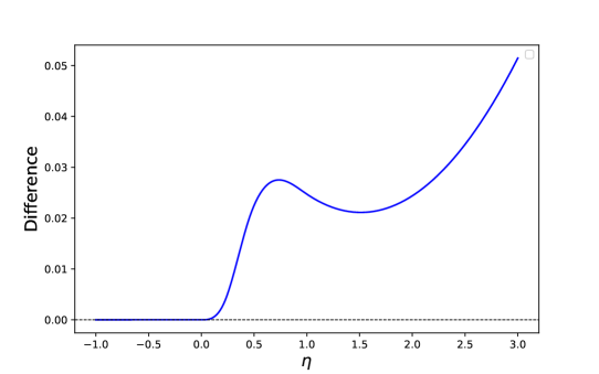
By standard calculation, one can check that $\mathbb{E}[\left(\eta-X\right)_{+}^{3}]\leq\mathbb{E}[\left(\eta-Y\right)_{+}^{3}]$ for all $\eta\in\mathbb{R}$ (see Figure 1 for an intuitive illustration), which implies that $X\not\geq_{4}Y$ . Moreover,

\displaystyle\mathbb{E}\left[\left(2-X\right)^{2}\right]-\mathbb{E}\left[\left(2-Y\right)^{2}\right]=-\frac{13}{2916}<0.

Hence, we also have $X\not\geq_{4}^{[0,2]}Y$ .

The next result examines the consistency of $n{\rm SD}$ when applied across various intervals. Notably, $n{\rm SD}_{[a,b]}$ does not depend on $a$ as long as $a$ is smaller than the left endpoint of the support of the random variables to compare. For simplicity, we assume that the left endpoint of all intervals is the same in the following theorem.

Theorem 1.

Fix $a,b,c,d\in\mathbb{R}$ with $a<b\leq c<d$ and $n\in\mathbb{N}$ .

\displaystyle\mbox{For all $X,Y\in\mathcal{X}_{[a,b]}$}:X\geq_{n}^{[a,c]}Y~{}\Longrightarrow~{}X\geq_{n}^{[a,d]}Y.

(2)

The backward implication of (2) holds if and only if $n\leq 3$ .

Theorem 1 illustrates that the ranking of two random variables can be inconsistent when applying $n$ SD across different intervals when $n\geq 4$ . Specifically, when two stochastic dominance relations, defined over intervals $A$ and $B$ such that the right endpoint of $B$ exceeds that of $A$ , this inconsistency arises. Importantly, such inconsistencies occur even when only considering random variables whose support is confined to a sub-interval of $A\cap B$ , not necessarily the entire intersection.

In practice, the exact interval that bounds all possible values of wealth may not be known, and decision makers typically set a sufficiently large range based on historical data. Suppose that there are two risk analysts using 4SD to rank the stock returns in one year. One chooses $[-100\%,2000\%]$ as the reference interval, and one chooses $[-100\%,1000\%]$ as the reference interval. Consider two stock returns, denoted by $X$ and $Y$ , evaluated based on their historical performance, both taking values between $[-1,1]$ . The first analyst may conclude that $X$ dominates $Y$ in 4SD, and the second may conclude that the domination does not hold. In this example, although both analysts choose very large upper bound $b$ for the interval that surely contains all possible values of $X$ and $Y$ , it is unclear which value of $b$ is the right one to choose, and this subjective choice affects their conclusion on domination. In extreme scenarios, where a new observation shows that the upper bound $b$ is not large enough to cover all risks of interest, the analysts must enlarge their interval, and may arrive at different domination relations even for those return variables that are within the originally chosen interval.

Proposition 1 can be generalized to include a broader category of stochastic dominance rules known as $n$ th degree $m$ -mean preserving stochastic dominance (Liu (2014)), denoted as $(n,m){\rm SD}_{[a,b]}$ . Specifically, for $X,Y\in\mathcal{X}_{[a,b]}$ , $X$ dominates $Y$ in $(n,m){\rm SD}_{[a,b]}$ if $X\geq_{n}^{[a,b]}Y$ and $F_{X}^{[k]}(b)\leq F_{Y}^{[k]}(b)$ for all $k\in[n]$ , with equality holding for all $k\in[m+1]$ . This concept can be extended to the set of all bounded random variables, denoted as $(n,m){\rm SD}_{\mathbb{R}}$ , where $X$ dominates $Y$ if $X\geq_{n}Y$ and $\mathbb{E}[X^{k}]=\mathbb{E}[Y^{k}]$ for each $k\in[m]$ . The higher-order stochastic dominance is a particular instance of $n$ th degree $m$ -mean preserving stochastic dominance with $m=0$ . If $m=1$ , this dominance criterion corresponds to $n$ th degree mean-preserving stochastic dominance as introduced in Denuit and Eeckhoudt (2013). When $m=n-1$ , it aligns with the notion of $n$ th degree risk increase as originally defined by Ekern (1980).

For the above two formulations of $n$ th degree $m$ -mean preserving stochastic dominance, we have the following result about the consistency that extends Proposition 1.

Theorem 2.

Let $a,b\in\mathbb{R}$ with $a<b$ and $m,n\in\mathbb{N}$ with $m\leq n-1$ .

\displaystyle\mbox{For all $X,Y\in\mathcal{X}_{[a,b]}$}:\mbox{ $X$ dominates $Y$ in $(n,m){\rm SD}_{[a,b]}$}~{}\Longrightarrow~{}\mbox{$X$ dominates $Y$ in $(n,m){\rm SD}_{\mathbb{R}}$}.

(3)

The backward implication of (3) holds if and only if $n-m\leq 3$ .

Theorem 2 shows that the $n$ th degree mean-preserving stochastic dominance rules are consistent for $n\leq 4$ . Furthermore, the $n$ th degree risk increase rules are always consistent across different intervals. This finding indicates that when a decision maker uses the $n$ th-degree risk increase rule to compare uncertain outcomes, she can uniformly apply its counterpart on $\mathbb{R}$ , making it suitable for all bounded uncertainty outcomes.

3 Proofs

3.1 Proof of Proposition 1

Note that $\overline{\mathcal{U}}_{n}^{[a,b]}$ is the closure of ${\mathcal{U}}_{n}^{[a,b]}$ with respect to pointwise convergence. We only need to consider the statements (i), (ii), (iv) and (v). Below we will prove Proposition 1 by three steps.

(a)

Prove (i) $\Leftrightarrow$ (iv) for $n\leq 3$ .
(b)

Prove (i) $\Leftrightarrow$ (ii) $\Rightarrow$ (iv) $\Leftrightarrow$ (v) for $n\in\mathbb{N}$ .
(c)

For any $c,d\in(-\infty,\infty)$ with $c<d$ and $n\geq 4$ , there exist $X,Y\in\mathcal{X}_{[c,d]}$ such that $X\geq_{n}Y$ and $X\not\geq_{n}^{[c,d]}Y$ .

In Step (b), the equivalence of (i) and (ii) was well-established, as discussed in Section 2. Specifically, the implication (i) $\Rightarrow$ (ii) can be shown by using integration by parts, greatly facilitated by the condition $F_{X}^{[k]}(b)\leq F_{Y}^{[k]}(b)$ for $k\in[n]$ derived from $X\geq_{n}^{[a,b]}Y$ . This condition, however, is absent in the analysis of the implication (iv) $\Rightarrow$ (v). In fact, the implication (iv) $\Rightarrow$ (v) can be verified by the insight that every $u\in\mathcal{U}_{n}$ is a positive linear combination of singularity functions in the set $\{f:x\mapsto-(\eta-x)_{+}^{n-1}|\eta\in\mathbb{R}\}$ ; see Williamson (1956). We provide a self-contained proof based on the integration by parts.

Before showing the proofs, we present an auxiliary lemma for later use.

Lemma 1 (Proposition 6 of Ogryczak and Ruszczyński (2001)).

For $Z\in\mathcal{X}$ and $n\in\mathbb{N}$ , we have

\displaystyle\lim_{\eta\to\infty}\left\{\eta-\left(\mathbb{E}[(\eta-Z)_{+}^{n}]\right)^{1/n}\right\}=\mathbb{E}[Z].

As a result, for $X,Y\in\mathcal{X}$ and $n\in\mathbb{N}$ , $X\geq_{n}Y$ implies $\mathbb{E}[X]\geq\mathbb{E}[Y]$ .

Proof of Step (a).

The cases $n\in\{1,2\}$ are trivial. Let now $n=3$ .

(i) $\Rightarrow$ (iv): It is straightforward to see that (i) implies $\mathbb{E}[(\eta-X)_{+}^{2}]\leq\mathbb{E}[(\eta-Y)_{+}^{2}]$ for all $\eta\in(-\infty,b]$ and $\mathbb{E}[X]\geq\mathbb{E}[Y]$ . For $\eta>b$ , we have

	$\displaystyle\mathbb{E}[(\eta-X)_{+}^{2}]$	$\displaystyle=\mathbb{E}[((b-X)+(\eta-b))^{2}]=\mathbb{E}[(b-X)^{2}]+2(\eta-b)\mathbb{E}[b-X]+(\eta-b)^{2}$
		$\displaystyle\leq\mathbb{E}[(b-Y)^{2}]+2(\eta-b)\mathbb{E}[b-Y]+(\eta-b)^{2}=\mathbb{E}[(\eta-Y)_{+}^{2}].$

This yields (iv).

(iv) $\Rightarrow$ (i): It follows from Lemma 1 that (iv) implies $\mathbb{E}[X]\geq\mathbb{E}[Y]$ . This completes the proof. ∎

Proof of Step (b).

The implication (i) $\Leftrightarrow$ (ii) has been verified in Theorem 1 of Eeckhoudt et al. (2009). The implication (ii) $\Rightarrow$ (v) is trivial. The implication (v) $\Rightarrow$ (iv) is supported by the fact that the mapping $x\mapsto-(\eta-x)_{+}^{n-1}$ is contained in $\overline{\mathcal{U}}_{n}$ , and thus, it can be approximated by the functions in $\mathcal{U}_{n}$ with respect to the pointwise convergence.

It remains to verify (iv) $\Rightarrow$ (v). To see this, suppose that $X\geq_{n}Y$ . It follows from Lemma 1 that $\mathbb{E}[X]\geq\mathbb{E}[Y]$ . First, we assume that $\mathbb{E}[X]>\mathbb{E}[Y]$ , and the case that $\mathbb{E}[X]=\mathbb{E}[Y]$ will be studied later. Using Lemma 1 again and noting that $\mathbb{E}[X]>\mathbb{E}[Y]$ , there exists $M\geq b$ such that $F_{X}^{[k]}(M)\leq F_{Y}^{[k]}(M)$ for all $k\in[n-1]$ . For $u\in\mathcal{U}_{n}$ , using integration by parts yields

	$\displaystyle\mathbb{E}[u(X)]-\mathbb{E}[u(Y)]$	$\displaystyle=\int_{\mathbb{R}}u(\eta)\mathrm{d}F_{X}(\eta)-\int_{\mathbb{R}}u(\eta)\mathrm{d}F_{Y}(\eta)$
		$\displaystyle=\int_{-\infty}^{M}(-1)u(\eta)\mathrm{d}\left(F_{Y}(\eta)-F_{X}(\eta)\right)$
		$\displaystyle=(-1)^{-1}u(\eta)(F_{Y}(\eta)-F_{X}(\eta))\big{\|}_{-\infty}^{M}+\int_{-\infty}^{M}(F_{Y}(\eta)-F_{X}(\eta))\mathrm{d}u(\eta)$
		$\displaystyle=\int_{-\infty}^{M}(F_{Y}(\eta)-F_{X}(\eta))\mathrm{d}u(\eta)$
		$\displaystyle=\int_{-\infty}^{M}u^{(1)}(\eta)\mathrm{d}\left(F_{Y}^{[2]}(\eta)-F_{X}^{[2]}(\eta)\right)$
		$\displaystyle=u^{(1)}(\eta)\left(F_{Y}^{[2]}(\eta)-F_{X}^{[2]}(\eta)\right)\big{\|}_{-\infty}^{M}+\int_{-\infty}^{M}\left(F_{Y}^{[2]}(\eta)-F_{X}^{[2]}(\eta)\right)\mathrm{d}\left(-u^{(1)}(\eta)\right)$
		$\displaystyle\geq\int_{-\infty}^{M}\left(F_{Y}^{[2]}(\eta)-F_{X}^{[2]}(\eta)\right)\mathrm{d}\left(-u^{(1)}(\eta)\right),$

where the inequality follows from $u^{(1)}\geq 0$ and $F_{X}^{[2]}(M)\leq F_{Y}^{[2]}(M)$ . Using integration by parts repeatedly following a similar argument, we get

\displaystyle\int_{-\infty}^{M}\left(F_{Y}^{[2]}(\eta)-F_{X}^{[2]}(\eta)\right)\mathrm{d}\left((-1)u^{(1)}(\eta)\right)

\displaystyle\geq\int_{-\infty}^{M}\left(F_{Y}^{[n]}(\eta)-F_{X}^{[n]}(\eta)\right)\mathrm{d}\left((-1)^{n-1}u^{(n-1)}(\eta)\right)\geq 0,

where the last inequality holds because $F_{X}^{[n]}(\eta)\leq F_{Y}^{[n]}(\eta)$ for all $\eta\in\mathbb{R}$ , and $(-1)^{n-1}u^{(n-1)}$ is increasing as $(-1)^{n-1}u^{(n)}\geq 0$ . Hence, we have $\mathbb{E}[u(X)]\geq\mathbb{E}[u(Y)]$ if $\mathbb{E}[X]>\mathbb{E}[Y]$ . Suppose now that $\mathbb{E}[X]=\mathbb{E}[Y]$ . It is straightforward that $X+\epsilon\geq_{n}Y$ for all $\epsilon>0$ . It follows from the previous arguments that $\mathbb{E}[u(X+\epsilon)]\geq\mathbb{E}[u(Y)]$ . Note that $\mathbb{E}[u(X+\epsilon)]\to\mathbb{E}[u(X)]$ as $\epsilon\downarrow 0$ . This gives $\mathbb{E}[u(X)]\geq\mathbb{E}[u(Y)]$ . Hence, we have completed the proof. ∎

Proof of Step (c).

Let us now focus on Step (c). To verify this step, it suffices to show that there exist $a,b\in(-\infty,\infty)$ with $a<b$ and $X,Y\in\mathcal{X}_{[a,b]}$ such that $X\geq_{4}Y$ and $X\not\geq_{4}^{[a,b]}Y$ , and such example has been given in Example 1. To see this, suppose that $X,Y\in\mathcal{X}_{[a,b]}$ are the random variables satisfying $X\geq_{4}Y$ and $X\not\geq_{4}^{[a,b]}Y$ . Then, we have $\mathbb{E}[(\eta-X)_{+}^{3}]\leq\mathbb{E}[(\eta-Y)_{+}^{3}]$ for all $\eta\in\mathbb{R}$ . It follows from Lemma 1 that $\mathbb{E}[b-X]\leq\mathbb{E}[b-Y]$ , and hence, $X\not\geq_{4}^{[a,b]}Y$ implies $\mathbb{E}[(b-X)^{2}]>\mathbb{E}[(b-Y)^{2}]$ . For $c,d\in(-\infty,\infty)$ with $c<d$ and $n\geq 4$ , define $\widetilde{X}=\lambda X+m$ and $\widetilde{Y}=\lambda Y+m$ , where $\lambda=(d-c)/(b-a)$ and $m=(bc-ad)/(b-a)$ . It is straightforward to see that $\widetilde{X},\widetilde{Y}\in\mathcal{X}_{[c,d]}$ , and $X\geq_{4}Y$ implies $\widetilde{X}\geq_{n}\widetilde{Y}$ . Additionally, we have

\displaystyle\mathbb{E}[(d-\widetilde{X})^{2}]=\lambda^{2}\mathbb{E}[(b-X)^{2}]>\lambda^{2}\mathbb{E}[(b-Y)^{2}]=\mathbb{E}[(d-\widetilde{Y})^{2}].

Therefore, we have concluded that $\widetilde{X},\widetilde{Y}\in\mathcal{X}_{[c,d]}$ , $\widetilde{X}\geq_{n}\widetilde{Y}$ and $\widetilde{X}\not\geq_{n}^{[c,d]}\widetilde{Y}$ , which confirms Step (c). Hence, we complete the proof. ∎

3.2 Proof of Theorem 1

We first present an auxiliary lemma.

Lemma 2.

Let $a,b\in\mathbb{R}$ with $a<b$ . There exists a sequence $\{X_{n},Y_{n}\}_{n\in\mathbb{N}}\subseteq\mathcal{X}_{[a,b]}^{2}$ such that $X_{n}\geq_{4}Y_{n}$ and $\mathbb{E}[X_{n}]-\mathbb{E}[Y_{n}]>0$ for all $n\in\mathbb{N}$ , and $(\mathbb{E}[X_{n}^{2}]-\mathbb{E}[Y_{n}^{2}])/(\mathbb{E}[X_{n}]-\mathbb{E}[Y_{n}])\to\infty$ .

Proof.

We assume without loss of generality that $a=0$ and $b=9$ . Let $\epsilon_{n}>0$ and $m_{n}\in(0,1)$ be such that $\epsilon_{n}=m_{n}/(54(1+m_{n}))$ and $m_{n}\downarrow 0$ . It holds that $m_{n}/\epsilon_{n}\downarrow 54$ as $n\to\infty$ . Define $\{X_{n},Y_{n}\}_{n\in\mathbb{N}}\subseteq\mathcal{X}_{[0,9]}^{2}$ with

\displaystyle F_{X_{n}}=\left(\frac{8}{9}+\epsilon_{n}\right)\delta_{2}+\left(\frac{1}{9}-\epsilon_{n}\right)\delta_{8+m_{n}}\mbox{~{}~{}and~{}~{}}F_{Y_{n}}=\frac{1}{3}\delta_{0}+\frac{2}{3}\delta_{4}.

It is straightforward to check that $\mathbb{E}[X_{n}]-\mathbb{E}[Y_{n}]=5\epsilon_{n}m_{n}>0$ for all $n\in\mathbb{N}$ . We aim to verify that $X_{n}\geq_{4}Y_{n}$ if $n\in\mathbb{N}$ is sufficiently large. To see this, denote by $f_{n}(\eta)=\mathbb{E}[(\eta-Y_{n})_{+}^{3}]-\mathbb{E}[(\eta-X_{n})_{+}^{3}]$ for $n\in\mathbb{N}$ and $\eta\in\mathbb{R}$ . It is straightforward to see that $f_{n}(\eta)\geq 0$ for $\eta\in(-\infty,4]$ . By standard calculation, we have

\displaystyle 9f_{n}(\eta)=g(\eta)-9\epsilon_{n}(\eta^{3}-6\eta^{2}+12\eta-8),~{}~{}\eta\in[4,8+m_{n}],

where $g(\eta)=\eta^{3}-24\eta^{2}+192\eta-320$ . One can check that the mapping $g(\eta)$ is increasing on $\mathbb{R}$ and $g(4)>0$ . Hence, we have $f_{n}(\eta)\geq g(4)-9\epsilon_{n}(\eta^{3}-6\eta^{2}+12\eta-8)$ for $\eta\in[4,8+m_{n}]$ . For sufficiently large $n$ , we have $\epsilon_{n}$ is small enough, and thus, $f_{n}(\eta)\geq 0$ for $\eta\in[4,8+m_{n}]$ . Let us now consider the case $\eta\geq 8+m_{n}$ . Denote by $A_{n}=(1-9\epsilon_{n})(6+m_{n})$ , and it holds that $A_{n}-6=5m_{n}^{2}/(6(1+m_{n}))>0$ and $A_{n}\to 6$ as $n\to\infty$ . By some standard calculations, we have

	$\displaystyle 9f_{n}(\eta)$	$\displaystyle=3(A_{n}-6)\eta^{2}+3[60-A_{n}(10+m_{n})]\eta+A_{n}(m_{n}^{2}+18m_{n}+84)-312$
		$\displaystyle\geq-\frac{3[A_{n}(10+m_{n})-60]^{2}}{4(A_{n}-6)}+A_{n}(m_{n}^{2}+18m_{n}+84)-312$
		$\displaystyle=-\frac{3}{4}\left[(10-m_{n})\sqrt{A_{n}-6}-\frac{6m_{n}}{\sqrt{A_{n}-6}}\right]^{2}+A_{n}(m_{n}^{2}+18m_{n}+84)-312$
		$\displaystyle\to-\frac{3}{4}\lim_{n\to\infty}\frac{36m_{n}^{2}}{A_{n}-6}+200=-\frac{162}{5}+200>0,$

where we have calculated the minimum of a quadratic function in the the first inequality by noting that $A_{n}>6$ , which implies that $f_{n}(\eta)>0$ for $\eta\geq 8+m_{n}$ when $n$ is sufficiently large. Therefore, we have concluded that $X_{n}\geq_{4}Y_{n}$ if $n\in\mathbb{N}$ is sufficiently large. Note that

	$\displaystyle\frac{\mathbb{E}[X_{n}^{2}]-\mathbb{E}[Y_{n}^{2}]}{\mathbb{E}[X_{n}]-\mathbb{E}[Y_{n}]}$	$\displaystyle=\frac{-9\epsilon_{n}m_{n}^{2}+m_{n}^{2}-144\epsilon_{n}m_{n}+16m_{n}-540\epsilon_{n}}{m_{n}-9\epsilon_{n}m_{n}-54\epsilon_{n}}$
		$\displaystyle=\frac{16\frac{m_{n}}{\epsilon_{n}}-540-9m_{n}^{2}+\frac{m_{n}^{2}}{\epsilon_{n}}-144m_{n}}{45m_{n}}\to\infty~{}~{}{\rm as}~{}n\to\infty,$

where the convergence follows from $m_{n}\downarrow 0$ and $m_{n}/\epsilon_{n}\downarrow 54$ . This comletes the proof. ∎

Proof of Theorem 1.

The implication in (2) follows from the equivalence between (i) and (ii) in Proposition 1. Note that the equivalence between (i) and (iii) in Proposition 1 holds for $n\leq 3$ , and thus, the backward implication of (2) also holds when $n\leq 3$ . It remains to verify that the backward implication fails if $n\geq 4$ . To see this, we assume without loss of generality that $a=0$ . Let $X,Y\in\mathcal{X}_{[0,b]}$ be such that $\mathbb{E}[X]>\mathbb{E}[Y]$ ,

\displaystyle X\geq_{4}Y~{}~{}{\rm and}~{}~{}\lambda:=\frac{\mathbb{E}[X^{2}]-\mathbb{E}[Y^{2}]}{\mathbb{E}[X]-\mathbb{E}[Y]}\geq 2d,

where the existence is due to Lemma 2. Let $\gamma\in(2c/\lambda,2d/\lambda]\subseteq(0,1]$ , and define $\widetilde{X}=\gamma X$ and $\widetilde{Y}=\gamma Y$ . It holds that $\widetilde{X},\widetilde{Y}\in\mathcal{X}_{[0,b]}$ , $\mathbb{E}[\widetilde{X}]>\mathbb{E}[\widetilde{Y}]$ ,

\displaystyle\widetilde{X}\geq_{4}\widetilde{Y}~{}~{}{\rm and}~{}~{}\frac{\mathbb{E}[\widetilde{X}^{2}]-\mathbb{E}[\widetilde{Y}^{2}]}{\mathbb{E}[\widetilde{X}]-\mathbb{E}[\widetilde{Y}]}=\gamma\frac{\mathbb{E}[X^{2}]-\mathbb{E}[Y^{2}]}{\mathbb{E}[X]-\mathbb{E}[Y]}\in(2c,2d].

Therefore, we have

	$\displaystyle\mathbb{E}[(c-\widetilde{X})^{2}]-\mathbb{E}[(c-\widetilde{Y})^{2}]=(\mathbb{E}[\widetilde{X}]-\mathbb{E}[\widetilde{Y}])\left(\frac{\mathbb{E}[\widetilde{X}^{2}]-\mathbb{E}[\widetilde{Y}^{2}]}{\mathbb{E}[\widetilde{X}]-\mathbb{E}[\widetilde{Y}]}-2c\right)>0;$
	$\displaystyle\mathbb{E}[(d-\widetilde{X})^{2}]-\mathbb{E}[(d-\widetilde{Y})^{2}]=(\mathbb{E}[\widetilde{X}]-\mathbb{E}[\widetilde{Y}])\left(\frac{\mathbb{E}[\widetilde{X}^{2}]-\mathbb{E}[\widetilde{Y}^{2}]}{\mathbb{E}[\widetilde{X}]-\mathbb{E}[\widetilde{Y}]}-2d\right)\leq 0.$

This implies that $\widetilde{X}\geq_{4}^{[0,d]}\widetilde{Y}$ and $\widetilde{X}\not\geq_{n}^{[0,c]}\widetilde{Y}$ for $n\geq 4$ . Since $\geq_{4}^{[0,d]}$ is more stringent than $\geq_{n}^{[0,d]}$ for $n\geq 4$ , we have completed the proof. ∎

3.3 Proof of Theorem 2

In this section, closure refers specifically to pointwise convergence. For $n\geq 3$ , define the class of $n$ -concave functions on $[a,b]$ as follows

\displaystyle\mathcal{U}_{n\text{-cv}}^{[a,b]}=\{u:\mathbb{R}\to\mathbb{R}|\mbox{$(-1)^{n-2}u^{(n-2)}$ is increasing and concave on $[a,b]$}\}.

The set $\mathcal{U}_{n\text{-cv}}^{[a,b]}$ is a closed convex cone. For any $u\in\mathcal{U}_{n\text{-cv}}^{[a,b]}$ , there exists a sequence $\{u_{k}\}_{k\in\mathbb{N}}$ such that $(-1)^{n}u_{k}^{(n)}\leq 0$ on $[a,b]$ for all $k\in\mathbb{N}$ and $u_{k}\to u$ pointwisely. Denote by $\mathcal{U}_{(n,m)\text{-cv}}^{[a,b]}=\bigcap_{i=m+1}^{n}\mathcal{U}_{i\text{-cv}}^{[a,b]}$ , which is also a closed convex cone. The following result is straightforward to verify by sharing a similar proof of Proposition 1 (see also Theorem 1 of Liu (2014)).

Lemma 3.

Let $a,b\in[-\infty,\infty]$ with $a<b$ and $m,n\in\mathbb{N}$ with $m\leq n-1$ . For $X,Y\in\mathcal{X}_{[a,b]}$ , $X$ dominates $Y$ in $(n,m){\rm SD}_{[a,b]}$ if and only if $\mathbb{E}[u(X)]\geq\mathbb{E}[u(Y)]$ for all $u\in\mathcal{U}_{(n,m)\text{-\rm cv}}^{[a,b]}$ .

Note that $\mathcal{U}_{(n,m)\text{-cv}}^{\mathbb{R}}\subseteq\mathcal{U}_{(n,m)\text{-cv}}^{[a,b]}$ whenever $a,b\in\mathbb{R}$ and $a<b$ . Hence, Lemma 3 yields (3) in Theorem 2.

Next, we aim to show that the backward implication of (3) holds if $n-m\leq 3$ . To see this, suppose that $X,Y\in\mathcal{X}_{[a,b]}$ satisfy that $X$ dominates $Y$ in $(n,m){\rm SD}_{\mathbb{R}}$ . The cases $n-m\in\{1,2\}$ are trivial. Let now $n-m=3$ . It suffices to verify that $\mathbb{E}[(b-X)^{m+1}]\leq\mathbb{E}[(b-Y)^{m+1}]$ . Since $X$ dominates $Y$ in $(n,m){\rm SD}_{\mathbb{R}}$ , we have $X\geq_{n}Y$ . Also note that $\mathbb{E}[X^{k}]=\mathbb{E}[Y^{k}]$ for $k\in[m]$ . By Theorem 4.A.58 of Shaked and Shanthikumar (2007), either $\mathbb{E}[X^{m+1}]=\mathbb{E}[Y^{m+1}]$ or $(-1)^{m+1}\mathbb{E}[X^{m+1}]<(-1)^{m+1}\mathbb{E}[Y^{m+1}]$ holds, which further implies that $\mathbb{E}[(b-X)^{m+1}]\leq\mathbb{E}[(b-Y)^{m+1}]$ . This completes the proof of the backward implication of (3) for $n-m\leq 3$ .

It remains to verify that the backward implication of (3) fails when $n-m\geq 4$ . Unlike in Proposition 1, where a counterexample is presented, here we seek to demonstrate this result through an alternative approach. Such an approach is based on the following lemma, which is a direct result from Corollary 3.8 of Müller (1997).

Lemma 4.

Let $a,b\in\mathbb{R}$ with $a<b$ , and let $\mathcal{V}_{1}$ and $\mathcal{V}_{2}$ be two closed convex cones of real-valued functions on $[a,b]$ . Suppose that $\succsim_{1}$ and $\succsim_{2}$ are two orderings on $\mathcal{X}_{[a,b]}$ , which satisfy for $X,Y\in\mathcal{X}_{[a,b]}$ and $i\in\{1,2\}$ , $X\succsim_{i}Y$ if and only if $\mathbb{E}[u(X)]\geq\mathbb{E}[u(Y)]$ for all $u\in\mathcal{V}_{i}$ . Then, the orderings $\succsim_{1}$ and $\succsim_{2}$ are equivalent if and only if $\mathcal{V}_{1}=\mathcal{V}_{2}$ .

We complete the proof by verifying that $(n,m){\rm SD}_{[a,b]}$ is a strictly more stringent rule than $(n,m){\rm SD}_{[a,c]}$ on $\mathcal{X}_{[a,b]}$ , where $a,b,c\in\mathbb{R}$ with $a<b<c$ and $m,n\in\mathbb{N}$ with $n-m\geq 4$ . Choose $u(x)=-(b-x)^{m+2}$ for $x\in\mathbb{R}$ . It is straightforward to see that $u\in\mathcal{U}_{(n,m)\text{-cv}}^{[a,b]}$ . Note that $\mathcal{U}_{(n,m)\text{-cv}}^{[a,b]}$ and $\mathcal{U}_{(n,m)\text{-cv}}^{[a,c]}$ are both closed convex cone. Combining Lemmas 3 and 4, it suffices to verify that $v\not\equiv u$ on $[a,b]$ for all $v\in\mathcal{U}_{(n,m)\text{-cv}}^{[a,c]}$ . To see this, we assume by contradiction that there exists $v\in\mathcal{U}_{(n,m)\text{-cv}}^{[a,c]}$ such that $v\equiv u$ on $[a,b]$ . It holds that

\displaystyle v^{(k)}(x)=u^{(k)}(x)=\frac{(-1)^{k+1}(m+2)!}{(m+2-k)!}(b-x)^{m+2-k}~{}~{}{\rm for}~{}x\in[a,b]~{}{\rm and}~{}k\in[m+2].

(4)

Define $f_{k}(x)=(-1)^{k}v^{(k)}(x)$ for $x\in[a,c]$ and $k\in[m+2]$ . We have that $f_{k}(x)$ is increasing and concave on $[a,c]$ for $k\in\{m-1,m,m+1,m+2\}$ as $v\in\mathcal{U}_{(n,m)\text{-cv}}^{[a,c]}$ with $n-m\geq 4$ . Note that $f_{m+2}(x)=-(m+2)!$ on $[a,b]$ , and thus, $f_{m+2}$ must be the constant $-(m+2)!$ on $[a,c]$ as it is increasing and concave. Further, the equation (4) implies $f_{m+1}(x)=-(m+2)!(b-x)$ for $x\in[a,b]$ . Since $f_{m+1}^{(1)}(x)=-f_{m+2}=(m+2)!$ for $x\in[a,c]$ , we have $f_{m+1}(x)=-(m+2)!(b-x)$ for $x\in[a,c]$ . This means that $f_{m+1}(x)>0$ for $x\in[b,c]$ . Note that $f_{m}^{(1)}(x)=-f_{m+1}(x)<0$ for $x\in[b,c]$ . This contradicts the fact that $f_{m}$ is increasing on $[a,c]$ . Hence, we have concluded that $(n,m){\rm SD}_{[a,b]}$ is a strictly more stringent rule than $(n,m){\rm SD}_{[a,c]}$ on $\mathcal{X}_{[a,b]}$ , where $a<b<c$ and $n-m\geq 4$ . This completes the proof.∎

4 Stochastic dominance on grids and sub-intervals

Many studies have explored stochastic dominance for distributions restricted to specific subsets of $\mathbb{R}$ , with several exploring the consistency of these orderings across various subsets. This section discusses some of them.

Fishburn (1976) investigated stochastic dominance on a restricted interval $[0,b]$ , defined such that $X$ dominates $Y$ if $F_{X}^{[n]}(\eta)\leq F_{Y}^{[n]}(\eta)$ for all $\eta$ within $[0,b]$ ³³3The order $n$ can take any real value from $[1,\infty)$ ; however, for our purposes, we consider only integer $n$ .. Compared to $n{\rm SD}_{[0,b]}$ , Fishburn’s criterion does not require the boundary condition at $b$ , making it less stringent than both $n{\rm SD}_{[0,b]}$ and $n{\rm SD}_{\mathbb{R}}$ . Furthermore, Fishburn (1980) showed that stochastic dominance relations in Fishburn (1976) align with $n{\rm SD}_{\mathbb{R}}$ only for $n\in\{1,2\}$ . In light of our Proposition 1, we conclude that $n{\rm SD}_{[0,b]}$ , $n{\rm SD}_{\mathbb{R}}$ , and Fishburn’s criterion exhibit consistent for $n=1$ and $n=2$ . However, for orders $n\geq 3$ , these criteria do not exhibit consistency.

The integral stochastic orderings (Whitt (1986); Müller (1997)) within a fixed subset of $\mathbb{R}$ , specifying that $X$ dominants $Y$ if $\mathbb{E}[u(X)]\geq\mathbb{E}[u(Y)]$ for all functions $u$ , which is defined on the subset, in a particular class $\mathcal{F}$ . Following this framework, Denuit et al. (1999) and subsequent works by Fishburn and Lavalle (1995) and Denuit and Lefevre (1997) explored stochastic orderings by setting the subset as a grid to compare discrete distributions. In particular, Denuit et al. (1999) showed that the ranking of two discrete distributions, each of the support is contained in a fixed grid, can become inconsistent when stochastic orderings are applied to the original grid and then extended to include an additional point. This inconsistency indicates that the choice of the grid significantly affects the ranking of random variables.

Denuit et al. (1998) and Denuit et al. (1999) studied $n$ -concave orderings within specific intervals, which correspond to increasing $n$ th-degree risk as introduced in Ekern (1980). These orderings are always consistent across different intervals (see our Theorem 2), enabling us to unify their use with the counterpart on $\mathbb{R}$ . Notably, Denuit et al. (1998) mentioned the possibility of inconsistencies between $n{\rm SD}$ and $n{\rm SD}_{[a,b]}$ in their Remark 3.6, but they did not provide explicit counterexamples or a detailed analysis. Our research builds on these observations and directly addresses these gaps, providing clarification of these potential inconsistencies.

References

Baiardi et al. (2020) Baiardi, D., Magnani, M. and Menegatti, M. (2020). The theory of precautionary saving: an overview of recent developments. Review of Economics of the Household, 18, 513–542.
Caballé and Pomansky (1996) Caballé, J. and Pomansky, A. (1996). Mixed risk aversion. Journal of Economic Theory, 71(2), 485–513.
Crainich et al. (2013) Crainich, D., Eeckhoudt, L. and Trannoy, A. (2013). Even (mixed) risk lovers are prudent. American Economic Review, 103(4), 1529–1535.
Deck and Schlesinger (2014) Deck, C. and Schlesinger, H. (2014). Consistency of higher order risk preferences. Econometrica, 82(5), 1913–1943.
Denuit and Eeckhoudt (2010) Denuit, M. and Eeckhoudt, L. (2010). Stronger measures of higher-order risk attitudes. Journal of Economic Theory, 145(5), 2027–2036.
Denuit and Eeckhoudt (2013) Denuit, M. and Eeckhoudt, L. (2013). Risk attitudes and the value of risk transformations. Journal of Economic Theory, 9(3), 245–254.
Denuit and Lefevre (1997) Denuit, M. and Lefevre, C. (1997). Some new classes of stochastic order relations among arithmetic random variables, with applications in actuarial sciences. Insurance: Mathematics and Economics, 20(3), 197–213.
Denuit et al. (1998) Denuit, M., Lefevre, C. and Shaked, M. (1998). The $s$ -convex orders among real random variables, with applications. Mathematical Inequalities and Applications, 1(4), 585–613.
Denuit et al. (1999) Denuit, M., Lefevre, C. and Utev, S. (1999). Stochastic orderings of convex/concave-type on an arbitrary grid. Mathematics of Operations Research, 24(4), 835–846.
Denuit et al. (1999) Denuit, M., De Vylder, E. and Lefevre, C. (1999). Extremal generators and extremal distributions for the continuous s-convex stochastic orderings. Insurance: Mathematics and Economics, 24(3), 201–217.
Eeckhoudt and Schlesinger (2006) Eeckhoudt, L. and Schlesinger, H. (2006). Putting risk in its proper place. American Economic Review, 96(1), 280–289.
Eeckhoudt et al. (2009) Eeckhoudt, L., Schlesinger, H. and Tsetlin, I. (2009). Apportioning of risks via stochastic dominance. Journal of Economic Theory, 144(3), 994–1003.
Ekern (1980) Ekern, S. (1980). Increasing $N$ th degree risk. Economics Letters, 6, 329–333.
Fang and Post (2022) Fang, Y. and Post, T. (2022). Optimal portfolio choice for higher-order risk averters. Journal of Banking and Finance, 137, 106429.
Fishburn (1976) Fishburn, P. C. (1976). Continua of stochastic dominance relations for bounded probability distributions. Journal of Mathematical Economics, 3(3), 295–311.
Fishburn (1980) Fishburn, P. C. (1980). Continua of stochastic dominance relations for unbounded probability distributions. Journal of Mathematical Economics, 7(3), 271–285.
Fishburn and Lavalle (1995) Fishburn, P. C. and Lavalle, I. H. (1995). Stochastic dominance on unidimensional grids. Mathematics of Operations Research, 20(3), 513–525.
Jean (1980) Jean, W. H. (1980). The geometric mean and stochastic dominance. The Journal of Finance, 35(1), 151–158.
Kimball (1990) Kimball, M. S. (1989). Precautionary saving in the small and in the large. Econometrica, 58(1), 53–73.
Kimball (1992) Kimball, M. S. (1992). Precautionary motives for holding assets. In G. Hubbard (Ed.), Asymmetric Information, Corporate Finance, and Investment. University of Chicago Press.
Levy (2015) Levy, H. (2015). Stochastic Dominance: Investment Decision Making under Uncertainty. Third Edition. Springer New York.
Liu (2014) Liu, L. (2014). Precautionary saving in the large: $n$ th degree deteriorations in future income. Journal of Mathematical Economics, 52, 169–172.
Liu and Neilson (2019) Liu, L. and Neilson, W. S. (2019). Alternative approaches to comparative $n$ th-degree risk aversion. Management Science, 65(8), 3824–3834.
Müller (1997) Müller, A. (1997). Stochastic orders generated by integrals: A unified study. Advances in Applied probability, 29(2), 414–428.
Nocetti (2016) Nocetti, D. C. (2016). Robust comparative statics of risk changes. Management Science, 62(5), 1381–1392.
Noussair et al. (2014) Noussair, C. N., Trautmann, S. T. and Van de Kuilen, G. (2014). Higher order risk attitudes, demographics, and financial decisions. Review of Economic Studies, 81(1), 325–355.
Ogryczak and Ruszczyński (2001) Ogryczak, W. and Ruszczyński, A. (2001). On consistency of stochastic dominance and mean–semideviation models. Mathematical Programming, 89, 217–232.
Rolski (1976) Rolski, T. (1976). Order relations in the set of probability distribution functions and their applications in queueing theory. Dissertationes Mathematicae CXXXII. Warsaw, Poland: Polska Akademia Nauk, Instytut Matematyczny.
Rothschild and Stiglitz (1970) Rothschild, M. and Stiglitz, J. (1970). Increasing risk: I. A definition. Journal of Economic Theory, 2(3), 225–243.
Shaked and Shanthikumar (2007) Shaked, M. and Shanthikumar, J. G. (2007). Stochastic Orders. Springer New York.
Schoenberg (1938) Schoenberg, I. J. (1938). Metric spaces and completely monotone functions. Annals of Mathematics, 39(4), 811–841.
Whitt (1986) Whitt, W. (1986). Stochastic comparisons for non-Markov processes. Mathematics of Operations Research, 11(4), 608–618.
Williamson (1956) Williamson, R. E. (1956). Multiply monotone functions and their Laplace transforms. Duke Mathematical Journal, 23(2), 189–207.