[1]\fnmRadoslav \surHarman
[1]\orgdivFaculty of Mathematics, Physics and Informatics, \orgnameComenius University, \orgaddress\streetMlynská Dolina F1, \cityBratislava, \postcode842 48, \countrySlovakia
The Polytope of Optimal Approximate Designs: Extending the Selection of Informative Experiments
Abstract
Consider the problem of constructing an experimental design, optimal for estimating parameters of a given statistical model with respect to a chosen criterion. To address this problem, the literature usually provides a single solution. Often, however, there exists a rich set of optimal designs, and the knowledge of this set can lead to substantially greater freedom to select an appropriate experiment. In this paper, we demonstrate that the set of all optimal approximate designs generally corresponds to a polytope. Particularly important elements of the polytope are its vertices, which we call vertex optimal designs. We prove that the vertex optimal designs possess unique properties, such as small supports, and outline strategies for how they can facilitate the construction of suitable experiments. Moreover, we show that for a variety of situations it is possible to construct the vertex optimal designs with the assistance of a computer, by employing error-free rational-arithmetic calculations. In such cases the vertex optimal designs are exact, often closely related to known combinatorial designs. Using this approach, we were able to determine the polytope of optimal designs for some of the most common multifactor regression models, thereby extending the choice of informative experiments for a large variety of applications.
keywords:
Multifactor regression model, Optimal design of experiment, Polytope, Rational arithmetic, Vertex optimal design1 Introduction
The optimal design of experiments is an important area of theoretical and applied statistics (e.g., Fedorov [17], Pázman [41], Pukelsheim [44], Atkinson et al. [2], Dean et al. [13]), closely related to various fields of mathematics and computer science, such as probability theory, orthogonal arrays, network theory, machine learning and mathematical programming (e.g., Dette and Studden [12], Hedayat et al. [30], Ghosh et al. [24], He [28], Todd [53]). In fact, one of the aims of this paper is to initiate a deeper exploration of the relationships between optimal experimental design, the theory of multidimensional polytopes, and rational-arithmetic computation.
From a statistical perspective, an optimal design is an experimental plan that maximizes the information contained in the observations.111In the following section, we will rigorously define the technical terms and prove all important claims used in the introduction. The specific measure of information, called a criterion, depends on the goal of the experiment. The most prominent are the criteria of - and -optimality, both measuring the precision of the parameter estimation for the underlying statistical model.
We will primarily focus on “approximate” experimental design (also called designs “for infinite-sample size”, or “continuous” designs), introduced by Kiefer [33]. An approximate design specifies a finite set of experimental conditions, which is called the support of the design, and the proportions of trials performed at each of these conditions, referred to as the design weights. In contrast, an exact design determines integer numbers of trials for the support points; often, these integer numbers are obtained from the proportions dictated by an approximate design, by means of appropriate rounding. We will use the term “design”, without any qualifier, to denote specifically an approximate experimental design.
The literature provides analytic forms of optimal designs (i.e., their supports and weights) for many statistical models and criteria. The focus is usually on obtaining a single optimal design; however, there is often an infinite set of optimal designs.
Example 1.
Consider an experiment with continuous factors, the levels of which can be chosen anywhere within the interval . Assume that for different trials, the observations are independent, and at any combination of factor levels, the observation satisfies the standard linear regression model
| (1) |
where are the unknown parameters, and is an unobservable error with and . Let us choose the criterion of -optimality. Then, the uniform design that assigns of the trials to each of the factor level combinations in , i.e., an approximate-design analogue of the full factorial design with binary factors, is optimal. However, consider any and a design that assigns of the trials to each of the factor level combinations , , , , and of the trials to each of the factor level combinations , , , . It is simple to show that such a design is also optimal. That is, there is a continuum of optimal designs.
The knowledge of more than one optimal design can be of theoretical as well as practical significance: alternative optimal designs may facilitate the best choice of the actual experiment. Of particular interest are optimal designs with small supports, because they may be suitable for assessing measurement errors, can be less expensive to execute, and can be more easily rounded to efficient exact designs. However, an optimal design with a large support may sometimes be more appropriate, because it may for instance better allow for the assessment of lack of fit of the model. Therefore, our purpose is to analyze the set of all optimal designs for a given experimental design problem.
The available literature only provides sporadic results on the nonuniqueness of optimal design and on the selection of a particular optimal design. The fact that the optimal design is not always unique, and the problem of finding optimal designs with special characteristics, such as the “minimal” optimal designs, has already been mentioned by Kiefer [33] and Farrell et al. [16]. The term “absolutely” minimal optimal design was introduced by Farrell et al. [16] and later used by Pesotchinsky [42]. Next, Pesotchinsky [43] analyzed optimal designs for the quadratic regression on cubic regions and stated conditions for the uniqueness of the optimal design in this model.
In multifactor models, the simplest optimal design is often supported on a large product grid. For some models of this type, alternative optimal designs supported on smaller sets have been constructed (e.g., Corollary 3.5 in Cheng [8], Theorem 2.1 in Lim and Studden [36], page 378 in Pukelsheim [44] and Section 5 in Schwabe and Wong [51]). A result of Schwabe and Wierich [50] provides conditions that characterize all -optimal designs in additive multifactor models with constant term and without interactions via the -optimal designs in the single-factor models. Further, for the additive model in crossover designs, there can be a multitude of optimal designs, and Kushner [34] suggests searching for them using linear programming. Focusing on applications, Robinson and Anderson-Cook [46] analyze the situation when there are several exact -optimal screening designs and suggest choosing the suitable one subject to a secondary characteristic. More recently Rosa and Harman [48] employed linear programming to select optimal designs with small supports in the models with treatment and nuisance effects.
In this paper, unlike most of the optimal design literature, we do not solve the problem of constructing a single optimal design. Instead, we assume that we already have one, or that it can be easily constructed using theoretical or numerical methods. We demonstrate that for a given model and criterion, in cases where the optimal design is not unique, the set of all optimal designs is typically a polytope. Additionally, we provide various theoretical properties of this polytope. We show that its vertices, which we call vertex optimal designs, can not only be used to succinctly describe all other optimal designs, but themselves have various useful characteristics, such as small supports.
Example 2.
In Example 1, the uniform design on is a trivial -optimal design. However, the set of designs from Example 1 parametrized by is exactly the set of all -optimal designs for Model (1). That is, the polytope of optimal designs is a line segment, with two vertices. These vertices correspond to the two vertex optimal designs, defined by and ; they are the approximate design analogues of the two -optimal fractional factorial designs. The vertex optimal designs are the only minimal optimal designs. That is, they are the only optimal designs with the following property: in the sense of set inclusion, there is no optimal design with a smaller support. On the other hand, note that the support of any optimal design corresponding to is maximal in the sense that it covers the supports of all optimal designs.
As we will show, the polytope of optimal designs can be described in a relatively straightforward way as an intersection of halfspaces, which is called the H-representation of a polytope. However, enumerating the vertices of a polytope given by its H-representation generally requires extensive calculations. This is known as the vertex enumeration problem.
The vertex enumeration problem can be solved by the pivoting algorithms based on the simplex method of linear programming (e.g., Avis and Fukuda [4]) and the nonpivoting algorithms based on the double description method (Motzkin et al. [39], Avis and Jordan [5]). An overview of the vertex enumeration methods can be found in Matheiss and Rubin [38] or Chapter 8 in Fukuda [21]. In experimental design, the double description algorithm has been used by Snee [52] and by Coetzer and Haines [10] to compute the extreme points of the design space in Scheffè mixture models with multiple linear constraints. In He [29], the algorithm facilitated the construction of a special type of minimax space-filling designs.
Computationally, the general vertex enumeration problem is NP-complete (Khachiyan et al. [32]). Despite its theoretical complexity, a key property of this problem is that if the H-representation of the polytope involves only rational numbers, the coordinates of its vertices are also rational numbers. Moreover, in this case the vertex enumeration algorithms can execute all calculations via rational arithmetic, thus providing an error-free method of constructing the vertices (e.g., Fukuda [20]), which is akin to a computer-assisted proof. For a general exposition of error-free computing in geometric problems, see Eberly [14].
This fact has important consequences for the construction of vertex optimal designs of experiments. The reason is that for many optimal design problems, the H-representation of the optimal polytope is fully rational. Consequently, by employing the rational-arithmetic computations, we can provide a complete list of all vertex optimal designs for a variety of standard models and a large class of criteria, involving both - and -optimality. In addition, for the rational optimal design problems, the vertex optimal designs are exact, i.e., realizable with a finite number of trials. Often, they correspond to standard combinatorial designs of experiments.
It is also possible to apply floating-point versions of the vertex enumeration algorithms for arbitrary optimal design problems as a general algorithmic method of constructing the vertex optimal designs. However, the outputs of such algorithms are not always perfectly precise due to the nature of floating-point computations. Since our aim is to provide results that are completely reliable from the theoretical point of view, we only focus on rational optimal design problems.
The rest of this paper is organized as follows. Section 2.1 sets the background on the theory of optimal design. In Section 2.2, we introduce the notions of a maximal optimal design and maximum optimal support, which play important roles in the construction of the polytope of optimal designs. In Sections 2.3 and 2.4, we mathematically describe the optimal polytopes viewed as sets of finite-dimensional vectors and as finitely supported probability measures, respectively. Section 2.5 introduces the class of rational optimal design problems, for which it is possible to completely and reliably determine the optimal polytopes. Section 2.6 provides suggestions for utilizing the polytope of optimal designs for constructing experimental designs with specific properties. In Section 3, we characterize the polytopes of optimal designs for various common models and criteria. Section 4 offers concluding remarks, highlighting key insights of our findings and avenues for further study. Additionally, appendices include a reference list of the notation, all non-trivial proofs, and other supporting information.
2 Theory
2.1 Optimal design
Let be a compact design space, that is, the set of all design points available for the trials. Note that such a definition of includes both continuous and discrete spaces.
Consider a continuous function , , that defines a linear regression model on in the following sense: provided that the experimental conditions of a trial are determined by the design point , the observation is , where is a vector of unknown parameters, and is an unobservable random error with expected value and variance . The random errors across different trials are assumed to be independent.
We remark that we restrict ourselves to linear homoscedastic regression models only for simplicity; the results of this paper can also be applied to nonlinear regression models through the approach of local optimality and to cases of non-constant error variance by means of a simple model transformation (e.g., [2], Chapters 17 and 22).
As is usual in the optimal design literature (e.g., Section 1.24 in [44]), we will formalize an approximate design as a probability measure on with a finite support , where is the support size, and are the support points. The interpretation is that for any the number gives the proportion of the trials to be performed under the experimental conditions determined by the design point . For clarity, we will sometimes represent the design by the table
For a design , the normalized information matrix is the positive semi-definite matrix
which is of size . We will assume that the problem at hand is nondegenerate in the sense that there is a design such that is nonsingular.
The quality of the design is measured by the “size” of , assessed through a utility function known as a criterion. For simplicity,222It is straightforward to use the methods developed in this paper with any information function that is strictly concave in the sense of Section 5.2 in [44]. we will focus on Kiefer’s criteria with a parameter in their information-function versions, as defined in Chapter 6 of Pukelsheim [44]. For a singular , the value of the -criterion is , and for a non-singular it is defined by
This class includes the two most important criteria: -optimality () and -optimality (). We also implicitly cover the criterion of -optimality (also called - or -optimality), because the problem of -optimal design is equivalent to the problem of -optimal design in a linearly transformed model (e.g., Section 9.8 in Pukelsheim [44]).
For the chosen , the -optimal design is any design that maximizes in the set of all designs . Note that our assumptions imply that there exists at least one -optimal design.
The most important result on optimal approximate designs is the so-called equivalence theorem; for Kiefer’s criteria it states that a design is -optimal if and only if is non-singular and
| (2) |
with equality for all (e.g., Section 7.20 in Pukelsheim [44]). In addition, for several standard linear regression models (e.g., those analyzed in Sections 3.2, 3.3 and 3.4), there exists a simple design such that for some and
| (3) |
Then, by Corollary 4 of [26], the design is -optimal for all parameters .
Let be fixed. While there can be an infinite number of -optimal designs, the properties of the Kiefer’s criteria and the assumption of nondegeneracy imply that the information matrix of all -optimal designs is the same; see, e.g., Section 8.14 in Pukelsheim [44]. We will denote this unique and necessarily nonsingular -optimal information matrix by . In the rest of this paper, if the criterion is general, fixed, or known from the context, we will drop the prefix -.
Of particular importance are the notions of a minimal optimal design and an absolutely minimal optimal design, introduced by Farrell et al. [16]. An optimal design is a minimal optimal design if there is no optimal design, whose support is a proper subset of .333Some authors use the expression “minimally-supported design” to denote any design with the support size equal to the number of parameters (Chang and Lin [7], Li and Majumdar [35] and many others), which is a different concept. An optimal design is called an absolutely minimal optimal design if there is no optimal design, whose support has fewer elements than .
2.2 Maximum optimal support
As stated in the introduction, our aim is to characterize the set of all optimal designs, if we already know one optimal design. To this end, we will assume that we know a “maximal” optimal design , which we define as an optimal design satisfying for any other optimal design . We emphasize that in many models, such as those analysed in Section 3, the known and simplest optimal design satisfies
| (4) |
i.e, is maximal, owing to the equivalence theorem for -optimality.
Of course, for some optimal design problems, a maximal optimal design is not immediately apparent. Even then, it is usually possible to construct one by a procedure that inspects either the design points satisfying equality in (2), or the points of a theoretically derived finite set necessarily covering the supports of all optimal designs; see, e.g., Section 3 in [31] or Lemma 4.2 in [22].444Since there is a large variety of models with directly available maximal optimal designs to justify the broad applicability of our method, see Section 3, we decided not to detail such an inspection procedure or the theoretical results on possible supports of optimal designs in this paper. Note that some very specific models, such as the trigonometric regression on (Section 9.16 in Pukelsheim [44]), do not admit any maximal optimal design. This is because in these models the union of the supports of all optimal designs is an infinite set and, according to the standard definition we use, any design only has a finite support. We exclude such optimal design problems from our further considerations.
While there can be many maximal optimal designs, their supports must be the same; we will denote the unique “maximum optimal support” by , where is the size of the maximum optimal support, and the regressor vectors corresponding to the trials at by , for all .
Therefore, if our aim is to study only optimal designs, we can completely restrict our attention to the set and disregard the design points from . Let us henceforth denote by the set of all designs supported on .
Example 3.
Consider Model (1) from Examples 1 and 2. Here, the design space is ; that is, we have continuous factors. The regression function is for all , i.e., the number of parameters is . Let be the uniform design on the set with elements. A simple calculation yields . The design is optimal for any , because for all , which is equivalent to (2). In addition, we clearly have for all , which is a transcription of (4); hence, is a maximal optimal design, and is the maximum optimal support. All -optimal designs for Model (1) therefore belong to the set of designs supported on .
2.3 Polytope of optimal weights
Because is finite, any design in can be characterized by the weights that it assigns to the design points . We will call the vector of weights of . This correspondence allows us to work with vectors from instead of measures on . The components of each must be non-negative and sum to one; the set of all weight-vectors on is therefore the probability simplex . Analogously, given a vector of weights , the design determined by satisfies for all .
Because all optimal designs have the same information matrix, the set of all weight-vectors corresponding to the optimal designs is
where . Since is a bounded superset of , and the equalities are linear in , the set is a polytope555Because the definition of the term “polytope” somewhat varies across the mathematical literature, we remark that by polytope we mean a bounded convex polyhedron, i.e., a bounded intersection of closed half-spaces. For an introduction to the theory of polytopes, see, e.g., Ziegler [55]. in . Therefore, we will say that is the “polytope of optimal weights”. A compact expression of the polytope of optimal weights utilizes the matrix
where means the half-vectorization of a symmetric matrix. Therefore, the number of rows of A is .
Lemma 1.
The set of optimal design weights is
| (5) |
The proof of Lemma 1 requires showing that for some entails ; see Appendix B for the proofs. Note that (5) is geometrically the intersection of a finite number of halfspaces, that is, it is a H-representation of .
For the mathematical properties of the optimal design problem at hand, a key characteristic is the rank of , which we will call the “problem rank”. In the following lemma, “dimension” of a subset of a vector space refers to the affine dimension of its affine hull.
Lemma 2.
(a) The bounds for the problem rank are ; (b) The dimension of the set of the information matrices of all designs supported on is ; (c) The dimension of the polytope of optimal design weights is .
A simple consequence of Lemma 2 is that the polytope is trivial (), i.e., the optimal design is unique, if and only if , which is if and only if has full column rank. Note also that Lemma 2, parts (a) and (c), imply . It follows that for the case the polytope is trivial.
Because the dimension of is , belongs to some proper affine subspace of . However, we can transform to a full-dimensional polytope that has the same geometric properties (the number and incidence of the faces of all dimensions, the distance between vertices and so on), as follows.
Let , let the columns of form an orthonormal basis of the null space and let be a maximal optimal design with the vector of weights . Define an affine mapping at by . Note that the image of is the affine space , and its inverse on is . Therefore, is an affine bijection between and , which means that the geometric structure of is the same as the structure of
| (6) |
The interior of contains the origin . The full-dimensional polytope can be used for the numerical construction of specific optimal designs as outlined in Section 2.6, as well as for a visualization of the set of all optimal designs if .
Key elements of are its vertices. Note that the number of these vertices is finite; we will denote them . The representation (5) of is in fact in the standard form of the feasible set of a linear program. As such, the well-established theory of linear programming can be used to give the following characterizations of .
Theorem 1.
For let . The following statements are equivalent:
-
1.
is a vertex of , i.e., is the unique solution to the optimization problem for some .
-
2.
is an extreme point of , i.e., , and if are such that for then .
-
3.
, and the vectors are linearly independent.
-
4.
, and if is such that , then .
-
5.
, and if is such that , then .
Example 4.
Consider Model (1) from Examples 1-3, with the maximum optimal support and the optimal information matrix . Denote the elements of lexicographically as . By Lemma 1, , where the columns of are , . The full form of is provided as equation (24) in Appendix C. It is a matter of simple algebra to verify that the problem rank is . Consequently, part (c) of Lemma 2 implies that the dimension of is . Laborious but straightforward calculations show that all solutions to the system are , where , , and . Adding restricts the values of to the interval . Therefore, the elements of can be parametrized as , . Hence, is the line segment in with endpoints (vertices) and . Finally, since the vector of weights of a maximal optimal design is , has dimension , and its one-element orthonormal basis is , formula (6) yields that a full-dimensional “polytope” isomorphic to is the interval . For this simple problem, one can also directly verify the characterization of the vertices and given by Theorem 1.
2.4 Polytope of optimal designs
The central object of this paper is the set of all -optimal designs, i.e.,
Here we formulate corollaries of the results of Section 2.3 in the standard optimal design terminology, so that it is clear how these results translate from the weights to actual designs (i.e., finitely supported probability measures).
First, we show that the mathematical properties indeed translate to designs by formalizing the transformation as a linear isomorphism. Let be the linear space of all signed measures supported on . Clearly, is a linear one-to-one mapping between and , that is, a linear isomorphism, with inverse . Note that the image of in is , and the image of in is . The latter observation means that is isomorphic to ; we therefore call the “polytope of optimal designs”.
The Carathéodory theorem (e.g., [47], Section 17) says that for any bounded set , every point in the convex hull of can be expressed as a convex combination of at most points of . Taking Lemma 2 into account, we obtain:
Theorem 2.
For every design there is a design with the support size of at most , such that . In particular, there exists an optimal design supported on no more than points.
Theorem 2 is a strengthening of the standard “Carathéodory theorem” used in optimal design (e.g., Theorem 2.2.3 in Fedorov [17] or Section 8.2. in Pukelsheim [44]): we obtain the standard result for , but in general .
Recall that is the design determined by the weights and are the vertices of . We will call the corresponding designs , , the “vertex optimal designs” (VODs). In simpler terms, for each vertex of , , the uniquely determined vertex optimal design is
Since the mapping is a linear isomorphism between and , the role of the vertices in is analogous to the role of the VODs in .
As a consequence of Lemma 2 we see that the dimension of , understood as the dimension of its affine hull in , is . The knowledge of and the inequality provides another variant of the Carathéodory theorem expressed in terms of the VODs:
Theorem 3.
Any optimal design can be represented as a convex combination of VODs, where .
The main theorem characterizing the VODs, based directly on Theorem 1, is
Theorem 4.
The following statements are equivalent:
-
1.
is a vertex optimal design, i.e., is the unique solution to the optimization problem for some coefficients .
-
2.
is an extreme optimal design, i.e., , and if are such that for then .
-
3.
is an optimal design with “independent support information matrices”, i.e., , and the matrices , for , are linearly independent.
-
4.
is a minimal optimal design, i.e., , and if is such that , then .
-
5.
is a unique optimal design on , i.e., , and if is such that , then .
Note that Theorem 4, specifically part , implies that the support size of any VOD is between and . Theorem 4 also provides bounds on the number of the VODs in terms of the numbers , and ; see Appendix D.
Example 5.
Consider Model (1) from Examples 1-4. The vertices of the polytope of all optimal designs correspond to the design weights and derived in Example 4. That is, there are two VODs and , which are uniform on the sets and containing points , , , , and , , , , respectively. The set consists of designs , where , which assign the weight to all points of and the weight to all points of . One can easily see that the VODs and indeed satisfy all characterizations given by Theorem 4.
2.5 Rational optimal design problems
In Examples 3 to 5, we provided the complete characterization of the optimal design polytope via its vertices for Model (1). However, such analytical derivations become tedious with increasing number of factors and more complex models.
Fortunately, the problems of finding all VODs for many standard models (including Model (1)) are “rational”, that is, the polytope of optimal weights has a rational H-representation (5). More precisely, it means that the matrices and () have rational elements. These conditions are automatically satisfied if have rational elements, and the weights of at least one optimal design are rational numbers.
For a rational optimal design problem, all VODs have rational weights. Moreover, a rational optimal design problem allows for the use of error-free rational-arithmetic algorithms to construct the theoretical forms of all VODs. In Section 3, we therefore employ computer-assisted construction of VODs that are (analytically) optimal, rather than the manual construction of such designs.
The rational form of the weights of all VODs means that they are exact designs of some sizes . It is of theoretical interest that in the rational optimal design problems, any optimal approximate design is a convex combination of at most exact optimal designs; see Theorem 3. From the more practical point of view, the VODs can be combined to provide an entire pool of optimal designs that can be realized with a finite number of trials. In particular, for some we can achieve an exact design of any size that is a multiple of the greatest common divisor , cf. Nijenhuis and Wilf [40]. We illustrate this idea for all models analyzed in Section 3.
Finally, note that for a rational design problem, its rank can also be calculated in a perfectly reliable way using the rational arithmetic, even without the need to calculate the VODs. The problem rank alone provides the dimension of the set of all information matrices on (Lemma 2), an upper bound on the minimal support size (Theorem 2) and the dimension of the polytope of optimal designs (Lemma 2).
2.6 Specific optimal designs
Suppose that the optimal design is not unique, and we have the complete list of all VODs, characterizing the set of all optimal designs. Then we can select one or more optimal designs with special properties, to broaden the choice for the experimenter.
2.6.1 Optimal designs with small supports
Due to Theorem 4, the VODs exactly coincide with the minimal optimal designs. Since the set of VODs is finite, it is straightforward to determine all absolutely minimal optimal designs, by selecting the VODs with the smallest possible size of the support.
Special optimal designs with small supports can also be obtained by maximizing a strictly convex function over . Such a can only attain its maximum at one or more of the extreme points of ; by Theorem 4, these extreme points are exactly VODs. For instance, since the negative entropy
is strictly convex on , we are able to identify all minimum-entropy optimal designs by selecting the VODs with the smallest entropy.
There are numerous potential advantages to using optimal designs with small supports, as opposed to those with large supports: they can better facilitate replicated observations, are simpler and more economical to execute, and offer a more compact representation.
Another advantage of approximate designs with small supports, such as the VODs, is that they are generally more appropriate for the “rounding” algorithms, which convert approximate designs to the exact designs. For instance, the popular Efficient Rounding (see Pukelsheim and Rieder [45]) is only meaningful if the approximate design to be rounded has a support smaller than the required size of the exact design. The size of the support also appears in the formula for the lower bound on the efficiency of the resulting exact design, in the sense that the smaller the support, the better the bound (Section 7 in Pukelsheim and Rieder [45]).
Moreover, it is possible to “round” an optimal approximate design by applying an advanced mathematical programming method (e.g., Sagnol and Harman [49] or Ahipasaoglu [1]) at the support of an optimal approximate design, which generally provides better exact designs than Efficient Rounding. This approach can only be practically feasible if the associated optimization problem has a small number of variables, that is, if the support of the optimal approximate design is small.
2.6.2 Optimal designs with large supports
The list of all VODs also provides the complete characterization of all optimal designs whose support is maximum possible, i.e., with support . Recall that we call such designs maximal optimal designs. Every such design is of the form , where , ,
and vice-versa. For instance, we can construct a maximal optimal design with for all . In contrast to the minimally supported VODs, the set of all maximally-supported optimal designs corresponds to the relative interior of .
It is also often possible to select an optimal design with a large support by minimizing a convex function over . This can be performed by means of appropriate mathematical programming solvers applied to the problem
| (7) |
For instance, using solvers for convex optimization on under the appropriate linear constraints, we can obtain the unique maximum-entropy optimal design.
While it is possible to solve (7) without the knowledge of the vertices of , the vertices allow us to use two alternative approaches. First, applying the representation , see (6), we can solve the convex optimization problem
| (8) |
Here, the variable is -dimensional. Second, we can use the fact that the vertices of generate all optimal weights; therefore, we can solve the convex optimization problem
| (9) |
where the variable is -dimensional. For small or small , these two restatements can be much simpler problems than (7). For a demonstration, see Section 3.3.
Optimal designs with large supports can sometimes be preferable to those with small supports, because they offer a more comprehensive exploration of the design space and are more robust with respect to misspecifications of the statistical model. Additionally, they are sometimes mathematically simpler, exhibiting a higher degree of symmetry (cf. Section 5.1. in Harman et al. [27]).
2.6.3 Cost-efficient optimal designs
Finally, consider a linear cost function defined on :
where are the costs associated with the trial in . While a -minimizing optimal design can be computed by solving a problem of linear programming, the list of all VODs provides much more: a straightforward and complete characterization of the set of all optimal solutions. Indeed, let be the VODs that minimize . Then the set of all convex combinations of these designs is the set of all -minimizing optimal designs. Geometrically, the set of -minimizing optimal designs is always a face of (of some dimension between and ). For an illustration, see Section 3.2.
As a special case, we can directly obtain the range of the optimal weights at , for instance as a means to explore the possible costs associated with the trials at . For , the optimal weights , , range in the (possibly degenerate) interval
where is linear on . Note that the interval is in fact a one-dimensional projection of . Analogously, we can compute and visualize projections of of dimensions greater than , which can provide complete information on the possible ranges of subvectors of optimal weights; see Section 3.4 for illustrations of such projections.
3 Examples
In this section, we focus on optimal designs for several common regression models with factors. In each of these models, the uniform design on the maximum optimal support is a maximal optimal design (see Section 2.2). The size of grows superpolynomially with , while the number of parameters only grows polynomially. The standard Carathéodory theorem (cf. Theorem 2) implies that there always exists an optimal design with the support size of at most . Therefore, there exists some such that the optimal design is not unique for all .
Furthermore, each of the optimal design problems from this section is a rational problem (Section 2.5), as can be easily seen from the form of the model and the maximal optimal design. Therefore, we can use the rational arithmetic to identify the characteristics of the polytope of optimal designs, specifically its affine dimension and, most importantly, the sets of all VODs, cf. Sections 2.3 and 2.4.666We provide a description of the VODs for smaller than a limit determined by the capacity of our computational equipment. For some larger values of , we were only able to compute the rank of the problem, which provides the dimension of the polytope of optimal designs by Lemma 2.
For each model in this section, the minimum-entropy optimal designs (cf. Section 2.6.1) coincide with the absolutely minimal optimal designs, and the unique maximum-entropy optimal design (cf. Section 2.6.2) is the uniform design on .
Our calculations were performed with the help of the statistical software R; in particular, the rational polytope vertices were obtained using the packages Lucas et al. [37] and Geyer and Meeden [23]. We used a 64-bit Windows 11 system with an Intel Core i7-9750H processor operating at 2.60 GHz. The R codes and full detailed tables of all VODs from Section 3 are available upon request from the authors.
3.1 The first-degree model on without a constant term
Consider the model
| (10) | |||||
The case of a single factor () is trivial and for two factors (), all -optimal designs are unique; see Section 8.6 in Pukelsheim [44].
Let . For , let be the set of all vectors in with exactly components equal to . The following claims are straightforward to verify via (2) and (4); cf. Pukelsheim [44], page 376: If is odd, the maximum optimal support is for both - and -optimality. If is even, the maximum optimal support is for -optimality and for -optimality. For any , the design uniform on is maximal -optimal, and the design uniform on is maximal -optimal.
Consequently, it is possible to apply rational arithmetic calculations to prove that for the uniform optimal design on is the unique -optimal design, and the uniform design on is the unique -optimal design.
For and the -criterion, the dimension of is , and there are VODs. To describe the set of all VODs, consider two designs to be isomorphic, if they are the same up to a relabeling of the factors. Then, the VODs can be split into two classes of isomorphic designs. The first class consists of the VODs that are isomorphic to
| (11) |
All VODs in this class can be obtained by permuting the (first ) rows of the table. Note that permuting the columns corresponds to the same VOD. One of these VODs has been computed by integer quadratic programming as an exact -optimal design of size , ; see Table 1 in Filová and Harman [18]. For , these VODs are the absolutely minimal -optimal designs.
The second class of VODs for -optimality and consists of the VODs isomorphic to the uniform design
| (12) |
For and for the criterion of -optimality, has dimension , and there are VODs, all isomorphic to
| (13) |
One of these VODs has been identified by integer quadratic programming as an -optimal exact design of size , ; see Table 2 in Filová and Harman [18]. For , these VODs are the absolutely minimal -optimal designs. A -dimensional projection of and its vertices are depicted in Figure 1.

For , the sets of - and -optimal designs coincide. The dimension of is and it has vertices; their structure is similar to the case of -optimality for .
For and the criterion of optimality, it holds that the size of the maximum optimal support is , the problem rank is , and the dimension of is . For and the criterion of -optimality we have , and . We were not able to enumerate the individual VODs for this size.
Relations to block designs. For Model (10), a matrix of support points of a design on or can be viewed as the incidence matrix of a binary block design with treatments and blocks. In this view, the support points of the VODs isomorphic to (11) are partially balanced designs (PBDs; see Wilson [54]) with , , and . Here, is the common replication number, and the common concurrence. Similarly, the VODs isomorphic to (12) are PBDs with , , and . In addition, the support points of (13) correspond to a balanced incomplete block design (which is a PBD with a constant block size) for treatments, , , , and a common block size (cf. Pukelsheim [44], p. 378, Cheng [8]).
3.2 The first-degree model on without a constant term
In this section we consider the model
| (14) | |||||
where (the case is trivial). For this model, it is simple to see that the design uniform on satisfies , and use conditions (3) and (4) to verify that is a maximal optimal design with respect to all , ; that is, the polytope of optimal designs does not depend on the choice of the Kiefer’s criterion. The maximal optimal design is not uniquely optimal for any . Clearly, the optimal design problem is rational for any and we can employ rational-arithmetic calculations to derive the following characterizations.
For , the dimension of is , and there are VODs, each uniform on a two-point support. If we denote the elements of as , and , the VODs are uniform designs on the pairs , , and . These designs are the absolutely minimal optimal designs. They can be combined to construct exact optimal designs of sizes , .
For Model (14), we consider two designs to be isomorphic, if one can be obtained from the other one by any sequence of operations involving relabeling the factors, reverting the signs of any subset of the factors, and reverting all signs of the factors for any subset of the support points. For a design matrix representing a VOD, these operations mean permuting the rows, multiplying any set of rows by , and multiplying the factor levels of any set of columns by .
For , the dimension of is , and there are VODs, all isomorphic to
Note that the matrix of the support points is a submatrix of a Hadamard matrix. These VODs are the absolutely minimal optimal designs. They can be combined to construct a variety of optimal designs that are exact of sizes , .
For , the dimension of is , and there are VODs, all isomorphic to
The support points form a Hadamard matrix. In fact, the uniform design on the rows of any Hadamard matrix of order is a VOD and the support vectors of any VOD form a Hadamard matrix of order . These VODs are the absolutely minimal optimal designs. They can be combined to construct exact optimal designs of sizes , .
For , the dimension of is , and there are as many as VODs. Of these, are uniform designs on an -point support (i.e., they are exact of size ) and are nonuniform, supported on points (). They can be used to construct exact optimal designs of sizes for , .
For , the size of the maximum optimal support is , the problem rank is and the dimension of is ; for this size of the problem, the enumeration of the VODs was prohibitive for our computer equipment.
Designs minimizing a linear cost. As mentioned in Section 2.6.3, the list of all VODs allows us to completely describe the class of linear-cost minimizing optimal designs. Consider Model (14) with factors and assume that the cost of the trial in is , with any , where is the number of levels and is the number of levels in . It is a matter of simple enumeration to determine that the VOD
| (15) |
minimizes this cost, as does any of the VODs that can be obtained from (15) by relabeling the factors. However, the VOD
| (16) |
also minimizes this cost, as does any of the VODs that can be obtained from (16) by relabeling the factors. That is, the set of all cost-minimizing optimal designs is the set of all convex combinations of these VODs. Note that they provide exact optimal designs of sizes for , .
3.3 The first-degree model on
Here we consider the model
| (17) | |||||
for . For this model, it can again be readily shown that the design uniform on has the information matrix , and it is possible to use conditions (3) and (4) to verify that is a maximal optimal design with respect to all Kiefer’s criteria. Additionally, the optimal design problem itself is clearly rational.
The uniform design on is the unique optimal design if and . For , the dimension of is , and there are VODs, as described in Examples 1-5 for and . Both these VODs are exact designs of size , absolutely minimal optimal designs, and they can be combined to form exact optimal designs of sizes for any .
The situation is more complex for : the dimension of is , and there are VODs, which can be split into classes of isomorphic designs. The first subclass includes uniform designs isomorphic to
This matrix of support points is formed by concatenating a normalized Hadamard matrix of order and the matrix constructed from by reverting the signs of the first row. Its transpose forms an orthogonal array with two levels of strength .
The second class of VODs consists of two designs isomorphic to the uniform design
This support matrix can be constructed as . Its transpose forms an orthogonal array of strength . The VODs belonging to these two classes of uniform designs supported on points are the absolutely minimal optimal designs.
The third class of isomorphic VODs for contains designs, which are no longer uniform. They are all isomorphic to the following design supported on points:
If the point with weight were to be replicated twice, then the support points would form a transpose of a orthogonal array with two levels of strength . The VODs for provide exact designs of sizes , , .
For , the dimension of is , and the number of VODs is . The support sizes of the VODs are (they are all exact designs of size ), (), (), (), (), and (). The VODs can be combined to provide exact designs of sizes , , .
For , the size of the maximum optimal support is , the problem rank is and the dimension of is . The enumeration of the VODs for exceeded the capabilities of our computer equipment.
Optimal designs minimizing a convex function. To illustrate the search for an optimal design that minimizes a convex function (cf. Section 2.6.2), consider Model (17) with and the problem
| (18) |
where are given coefficients, and , i.e., the negative criterion of -optimality. The problem (18) can be interpreted as optimizing on in a heteroscedastic version of (17), with variances of the observations in proportional to . An alternative interpretation is optimizing on in (18) for proportions of failed trials in .
For illustration, we chose the coefficients for , for all four that contain one level , for all six that contain two levels , for all four that contain three levels and for .
We formulated (18) in the form (8) based on . Instead of this form, one can also use the forms (7) or (9), but our version works with , whereas (7) is based on and (9) is based on . Moreover, (8) requires maximizing a concave function over a feasible set with a guaranteed interior point . This allowed us to solve the problem with a function as simple as constrOptim of R. This procedure provided the design
3.4 The first-degree model on with second-order interactions
Consider the model
| (19) | |||||
where is the number of factors, and is the number of parameters. Model (19) is again a rational model, and the design uniform on satisfying is a maximal -optimal design for any , as can be confirmed by verifying conditions (3) and (4). It is the unique optimal design for .
However, for , an infinite number of optimal designs already exist; the dimension of is , and there are VODs, mutually isomorphic. One of these two VODs is the uniform design
Its support points form the transpose of a orthogonal array of strength . Both of these VODs are absolutely minimal optimal designs. They can be combined to obtain exact optimal designs of sizes , .
For , the dimension of is and there are VODs. The visualizations of selected -dimensional projections of the corresponding are in Figure 2. Of these VODs, are uniform on a -point support (exact of sizes ), and are nonuniform on a -point support (). Combining these VODs yields exact optimal designs of sizes and for all .

The computations were prohibitive for Model (19) with .
3.5 The additive second-degree model on
As the last example, we consider the model
| (20) | |||||
where , and the number of parameters is . Model (20) is rational for -optimality, as it is possible to verify that the uniform design on is a maximal -optimal777For this model, we consider only the criterion of -optimality, since analytic formulas of other -optimal designs for Model (20) with do not seem to be available in the literature, nor trivial to derive. design; cf. Pukelsheim [44] (Sections 9.5 and 9.9) for , and Schwabe and Wierich [50] for . For and , the uniform design on is the unique -optimal design.
However, for the dimension of the polytope of optimal designs is already and there are VODs. First, there are VODs, uniform on points, which form two distinct isomorphism classes. A representative of the members of the first class of VODs is the design
| (21) |
A representative of the members of the second class of VODs is the design
| (22) |
The support points of these VODs form the transpose of an orthogonal array of strength with levels and factors. The nice geometric properties of these designs are apparent from Figure 3. These VODs are absolutely minimal optimal designs.
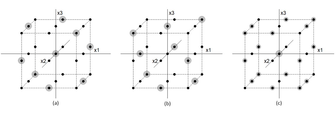
The remaining VODs are all designs supported on design points from , such that of these points have weight , one point has weight , and the projections to all three two-dimensional sub-spaces of these designs are uniform on the grid. They form distinct isomorphism classes which we will not detail. One of these VODs is
| (23) |
If the trial at were replicated twice, the matrix of the support points would form the transpose of an orthogonal array with levels of strength . The VODs for can be combined to obtain various exact optimal designs of sizes , .
As noted by one reviewer, Model (20) on can be linearly reparametrized as a main-effects ANOVA model with factors on levels each. Consequently, the -optimal designs in these two models should coincide. Indeed, it is possible to verify that the 3-dimensional projections of the widely used Taguchi L18 design for the ANOVA model form (some) -optimal designs for Model (20) with factors. These -optimal designs can be obtained as , where and are VODs from the two isomorphism classes represented by designs (21) and (22).
For , the size of the maximum optimal support is , the problem rank is , and the dimension of the polytope of optimal designs is . However, for the enumeration of the VODs was too time-consuming.
4 Conclusions
We brought attention to the fact that the set of all optimal approximate designs is generally a polytope. We have shown that its characteristics can be beneficial to both the theory and applications of experimental design. Particularly noteworthy are the vertices of this polytope – the vertex optimal designs – because of their several unique properties, especially their small supports, and the potential to generate all optimal designs.
Another key point is the application of a rational-arithmetic method that accurately identifies all vertex optimal designs for rational optimal design problems. The use of rational vertex enumeration methods is a new tool of constructing optimal approximate as well as optimal exact designs in an error-free manner, complementing the plethora of analytical techniques in the literature.
Importantly, we have obtained the vertex optimal designs for several commonly used models, thus providing complete information on the optimal approximate designs in these cases. We have demonstrated that in the studied cases, these designs, along with their combinations, correspond to exact optimal designs of various sizes, often related to block designs or orthogonal arrays.
To the best of our knowledge, this paper presents the first systematic approach to studying the set of all optimal designs, and it motivates a variety of intriguing topics for further research. For instance, it is possible to investigate the polytope of optimal designs for important non-rational design problems (including the optimal design problems for the full quadratic model with many factors) and less common statistical models, such as models for paired comparisons (e.g., [25]) or models with restricted design spaces (e.g., [19]). One can also explore extending the results to more specialized optimality criteria, such as those focusing on the estimation of a subset of parameters (see, for instance, Sections 10.2 to 10.5 in Atkinson et al. [2]). In addition, a general avenue of future research is the application of rational-arithmetic calculations in other problems of experimental design.
Acknowledgements We are grateful to Professor Rainer Schwabe from Otto von Guericke University Magdeburg and Associate Professor Martin Máčaj from Comenius University Bratislava for helpful discussions on some aspects of the paper. We would also like to thank the anonymous referees for their insightful comments that helped improve the paper.
Declarations
-
•
Funding. This work was supported by the Slovak Scientific Grant Agency (VEGA), Grant 1/0362/22.
-
•
Competing interests. The authors have no relevant financial or non-financial interests to disclose.
-
•
Ethics approval and consent to participate. Not applicable.
-
•
Consent for publication. Not applicable.
-
•
Data availability. Not applicable.
-
•
Materials availability. Not applicable.
-
•
Code availability. All codes used for the numerical results are available upon request from the authors.
-
•
Author contribution. All coauthors contributed to the conceptualization, methodology, mathematical proofs, software, writing and reviewing of the article.
Appendix A Notation
Below is an overview of the notation used throughout the paper and the appendices.
-
vector of all zeros
-
vector of all ones
-
components of a vector
-
identity matrix
-
column space of the matrix
-
null space of the matrix
-
trace of the matrix
-
determinant of the matrix
-
half-vectorization the matrix
-
transpose of , respectively
-
linear model
-
regression function
-
number of model parameters in
-
number of trials
-
design point
-
set of all design points, design space
-
(approximate) design
-
support of
-
information matrix of
-
Kiefer’s -criterion
-
optimal design
-
optimal information matrix
-
maximum optimal support
-
size of
-
elements of
-
-
design supported on
-
set of all designs supported on
-
set of all optimal designs
-
vector of design weights
-
support of
-
simplex of the weights of all designs on
-
polytope of all optimal weights
-
vector of weights corresponding to
-
design on with design weights
-
-
(number of rows of )
-
(problem rank)
-
(dimension of )
-
polytope in that is isomorphic to
-
number of vertices of , number of VODs
-
vertices of
-
vertext optimal designs (VODs)
-
number of factors
-
vectors in with ones
-
set for -optimality
-
set for -optimality
-
replication number, concurrence number, number of blocks of a partially balanced design
-
Hadamard matrix of order
Appendix B Proofs
B.1 Proof of Lemma 1.
Proof.
Let satisfy . Then , where the second equality follows form the basic properties of the trace, and the last equality follows from (2), i.e., from the equivalence theorem for all . As , we see that , i.e., . ∎
B.2 Proof of Lemma 2.
Proof.
(a): Because is a matrix, the second inequality is clear. To prove the first inequality, observe that since is nonsingular, span ; i.e., there exist linearly independent ’s. Without loss of generality assume that are linearly independent. We shall prove that the matrices are then also linearly independent (in the space of all matrices):
Let for some . This can be expressed as , where , and is the diagonal matrix with on the diagonal.
Because are linearly independent, is an non-singular matrix. Therefore , where we used the fact that the multiplication by a non-singular matrix preserves rank. It follows that ; i.e., , which proves the linear independence of .
Since is a linear isomorphism, it follows that are linearly independent, which implies .
(b): First note that (b) trivially holds when : then and the set contains just one matrix, so its dimension is . Suppose now that . Let , . The function is a linear isomorphism between and , so the dimension of is equal to the dimension of . The latter set is exactly the convex hull of , whose dimension is equal to the dimension of the affine hull of ; i.e., the dimension of . Observe that the linearity of vech gives and .
We will show that for any vector satisfying (even for with some negative components). If we denote and ), the fact that for all implies for all . For contradiction, suppose that there exists such that and . It follows that . Properties of then yield ; i.e., . This is, however, a contradiction, because .
As for any satisfying , we have for any such . It follows that is a strict subset of , which is . Therefore, the dimension of must be less than the dimension of the column space , which is . However, we can also write as (in the sense of the usual definition of the sum of two sets), which means that the dimension of is at least . Thus, the dimension of is exactly .
(c): Since the vector of weights that corresponds to the maximal optimal design satisfies and , the dimension of is the dimension of the null-space . From the rank-nullity theorem we therefore have that the dimension of is . ∎
B.3 Proof of Theorem 1.
Let . Then, can be expressed as
Now some notation used in the theory of linear programming needs to be introduced:
-
•
A constraint is any row in and any inequality ; i.e., is defined by constraints, where is the number of rows of .
-
•
A constraint is active at if it is satisfied as equality (that is, for the active constraints are all the constraints in , and all those constraints , for which ).
-
•
The vector is a basic solution if , and there are linearly independent constraints among all the constraints that are active at .
-
•
is a basic feasible solution if it is a basic solution and (i.e., if it also satisfies ).
Proof.
Theorem 2.3 by Bertsimas, Tsitsiklis [6] directly yields the equivalence of 1. and 2. That theorem also states that these are equivalent with being a basic feasible solution, and we shall show that this condition is equivalent to 4. and 5.
Let be a basic feasible solution, which means that there are linearly independent active constraints at . Let be the set of indices such that for . Then Theorem 2.2 by Bertsimas, Tsitsiklis [6] says that is the only vector that satisfies and for . Now let satisfy , that is for . It follows that because the solution to and for was unique; thus showing 4. Note that this also proves that if is a basic feasible solution, then it is the unique design supported on , i.e., it proves 5.
Conversely, let satisfy 4. and again denote as the set of indices for which . Now suppose that is not a basic solution, which means (in light of Theorem 2.2 by Bertsimas, Tsitsiklis [6]) that there exists such that and for (note that need not be satisfied outside ). However, any point that lies on the line going through and also satisfies , for . Now take as the point on this line that satisfies for and such that for some . Such can be constructed as the intersection of the line and the relative boundary of , and it exists because and for . This satisfies , which is in contradiction with 4. Note that if we assume 5. instead of 4., then constructed above is also in contradiction with 5. because it satisfies , but . This concludes the proof that is a basic feasible solution if and only if it satisfies either 4. or 5. Now Theorem 2.3 by Bertsimas, Tsitsiklis [6] gives the equivalence of 1., 4. and 5.
If , then Theorem 2.4 by Bertsimas, Tsitsiklis [6] yields that is a basic feasible solution if and only if it satisfies 3. However, the proof of that theorem can be easily extended to the case of of a general rank . It follows that 3. is equivalent to 4. and 5. ∎
Appendix C Ad Example 4
In Example 4, the full form of is
| (24) |
Appendix D Vertex bounds
If are two distinct vertex optimal designs (VODs), it follows that neither set nor can be a subset of the other, which follows from the part of Theorem 4. That is, the system of the supports of the VODs forms a Sperner family; this provides a simple upper limit on the number of the VODs via the Sperner’s theorem in terms of the simplest characteristic : . If we also know the problem rank or the dimension of , we can improve the Sperner’s bound as follows: since each -touple of independent elementary information matrices “supports” at most one VOD (see in Theorem 2), we have . For many situations, we can further improve the bound by using the H-representation of the full-dimensional isomporphic polytope and the McMullen’s Upper Bound Theorem (see, e.g., the introduction in Avis and Devroye [3]), which gives
On the other hand, since the support of each VOD must be at most , and any maximal optimal design must be a convex combination of some VODs, we must have . Also, since the dimension of is and the VODs generate , we must have .
Specifically, for (, ) we have (, ).
References
- Ahipasaoglu [2021] Ahipasaoglu SD (2021). A branch-and-bound algorithm for the exact optimal experimental design problem. Statistics and Computing 31, 1–11.
- Atkinson et al. [2007] Atkinson AC, Donev A, Tobias R (2007). Optimum experimental designs, with SAS. Oxford University Press.
- Avis and Devroye [2000] Avis D, Devroye L (2000). Estimating the number of vertices of a polyhedron. Information processing letters 73(3-4), 137–143.
- Avis and Fukuda [1996] Avis D, Fukuda K (1996). Reverse search for enumeration. Discrete applied mathematics 65(1-3), 21–46.
- Avis and Jordan [2015] Avis D, Jordan C (2015). Comparative computational results for some vertex and facet enumeration codes. arXiv preprint arXiv:1510.02545.
- Bertsimas, Tsitsiklis [1997] Bertsimas D, Tsitsiklis JN (1997). Introduction to Linear Optimization. Athena Scientific.
- Chang and Lin [2007] Chang FC, Lin HM (2007). On minimally-supported D-optimal designs for polynomial regression with log-concave weight function. Metrika 65, 227–233.
- Cheng [1987] Cheng CS (1987). An Application of the Kiefer-Wolfowitz Equivalence Theorem to a Problem in Hadamard Transform Optics. The Annals of Statistics 15, 1593–1603.
- Chernoff [1953] Chernoff H (1953). Locally optimal designs for estimating parameters. Ann. Math. Statist. 24, 586–602.
- Coetzer and Haines [2017] Coetzer R, Haines LM (2017). The construction of D-and I-optimal designs for mixture experiments with linear constraints on the components. Chemometrics and Intelligent Laboratory Systems 171, 112–124.
- Dantzig [1951] Dantzig GB (1951). Maximization of a linear function of variables subject to linear inequalities. Activity analysis of production and allocation 13, 339–347.
- Dette and Studden [1997] Dette H, Studden WJ (1997). The theory of canonical moments with applications in statistics, probability, and analysis. John Wiley & Sons.
- Dean et al. [2015] Dean AM, Morris M, Stufken J, Bingham D (Eds.) (2015). Handbook of design and analysis of experiments. Chapman & Hall/CRC.
- Eberly [2021] Eberly D (2021). Robust and error-free geometric computing. CRC Press.
- Elfving [1952] Elfving G (1952). Optimum allocation in linear regression theory. Annals of Mathematical Statistics 23, 255–262.
- Farrell et al. [1967] Farrell RH, Kiefer J, Walbran A (1967). Optimum multivariate designs. In Proceedings of the fifth Berkeley symposium on mathematical statistics and probability (Vol. 1, pp. 113-138). Berkeley, CA. University of California Press.
- Fedorov [1972] Fedorov VV (1972). Theory of optimal experiments. Academic Press.
- Filová and Harman [2020] Filová L, Harman R (2020). Ascent with quadratic assistance for the construction of exact experimental designs. Computational Statistics 35, 775–-801.
- Freise et al. [2020] Freise F, Holling H, Schwabe R (2020). Optimal designs for two-level main effects models on a restricted design region. Journal of Statistical Planning and Inference 204, 45–54.
- Fukuda [1997] Fukuda K (1997). cdd/cdd+ Reference Manual. Institute for Operations Research. ETH-Zentrum, 91–111.
- Fukuda [2020] Fukuda K (2020). Polyhedral computation. Department of Mathematics and Institute of Theoretical Computer Science, ETH Zurich. https://doi.org/10.3929/ethz-b-000426218
- Gaffke et al. [2014] Gaffke N, Graßhoff U, Schwabe R (2014). Algorithms for approximate linear regression design applied to a first order model with heteroscedasticity. Computational Statistics and Data Analysis 71, 1113–1123.
- Geyer and Meeden [2023] Geyer CJ, Meeden GD (2023). R package rcdd (C Double Description for R), version 1.5. https://CRAN.R-project.org/package=rcdd
- Ghosh et al. [2008] Ghosh A, Boyd S, Saberi A (2008). Minimizing Effective Resistance of a Graph. SIAM Review 50, 37–66.
- Graßhoff et al. [2004] Graßhoff U, Großmann H, Holling H, Schwabe R (2004). Optimal designs for main effects in linear paired comparison models. Journal of Statistical Planning and Inference 126, 361–376.
- Harman [2008] Harman R (2008). Equivalence theorem for Schur optimality of experimental designs. Journal of Statistical Planning and Inference 138, 1201–1209.
- Harman et al. [2020] Harman R, Filová L, Richtárik P (2020). A Randomized Exchange Algorithm for Computing Optimal Approximate Designs of Experiments. Journal of the American Statistical Association 115, 348–361.
- He [2010] He X (2010). Laplacian regularized D-optimal design for active learning and its application to image retrieval. IEEE Transactions on Image Processing 19, 254–263.
- He [2017] He X (2017). Interleaved lattice-based minimax distance designs. Biometrika 104(3), 713–725.
- Hedayat et al. [1999] Hedayat AS, Sloan NJA, Stufken J (1999). Orthogonal Arrays: Theory and Applications. Springer.
- Heiligers [1992] Heiligers B (1992). Admissible experimental designs in multiple polynomial regression. Journal of Statistical Planning and Inference, 31, 219–233.
- Khachiyan et al. [2009] Khachiyan L, Boros E, Borys K, Gurvich V, Elbassioni K (2009). Generating all vertices of a polyhedron is hard. In Twentieth Anniversary Volume: (pp. 1–17). Springer.
- Kiefer [1959] Kiefer J (1959). Optimum experimental designs. Journal of the Royal Statistical Society: Series B 21, 272–304.
- Kushner [1998] Kushner HB (1998). Optimal and efficient repeated-measurements designs for uncorrelated observations. Journal of the American Statistical Association 93(443), 1176–1187.
- Li and Majumdar [2008] Li G, Majumdar D (2008). D-optimal designs for logistic models with three and four parameters. Journal of Statistical Planning and Inference 138(7), 1950–1959.
- Lim and Studden [1988] Lim YB, Studden WJ (1988). Efficient Ds-optimal designs for Multivariate Polynomial Regression on the q-Cube. The Annals of Statistics 16(3), 1225–1240.
- Lucas et al. [2023] Lucas A, Scholz I, Boehme R, Jasson S, Maechler M (2023). R package gmp (Multiple Precision Arithmetic), version 0.7-2 https://CRAN.R-project.org/package=gmp
- Matheiss and Rubin [1980] Matheiss TH, Rubin DS (1980). A survey and comparison of methods for finding all vertices of convex polyhedral sets. Mathematics of operations research 5(2), 167–185.
- Motzkin et al. [1953] Motzkin TS, Raiffa H, Thompson GL, Thrall RM (1953). The double description method. Contributions to the Theory of Games 2(28), 51–73.
- Nijenhuis and Wilf [1972] Nijenhuis A, Wilf HS (1972). Representations of integers by linear forms in nonnegative integers. Journal of Number Theory 4, 98–106.
- Pázman [1986] Pázman A (1986). Foundation of Optimum Experimental Design. Reidel.
- Pesotchinsky [1975] Pesotchinsky LL (1975). D-optimum and quasi-D-optimum second-order designs on a cube. Biometrika 62(2), 335–340.
- Pesotchinsky [1978] Pesotchinsky L (1978). -optimal second order designs for symmetric regions. Journal of Statistical Planning and Inference 2(2), 173–188.
- Pukelsheim [1993] Pukelsheim F (1993). Optimal Design of Experiments. Wiley.
- Pukelsheim and Rieder [1992] Pukelsheim F, Rieder S (1992). Efficient rounding of approximate designs. Biometrika 79, 763–770.
- Robinson and Anderson-Cook [2010] Robinson TJ, Anderson-Cook CM (2010). A closer look at D-optimality for screening designs. Quality Engineering 23(1), 1–14.
- Rockafellar [1996] Rockafellar T (1996). Convex Analysis: Princeton Landmarks in Mathematics and Physics, 18, Princeton University Press
- Rosa and Harman [2016] Rosa S, Harman R (2016). Optimal approximate designs for estimating treatment contrasts resistant to nuisance effects. Statistical Papers 57, 1077–1106.
- Sagnol and Harman [2015] Sagnol G, Harman R (2015). Computing exact D-optimal designs by mixed integer second-order cone programming. The Annals of Statistics 43, 2198–-2224.
- Schwabe and Wierich [1995] Schwabe R, Wierich W (1995). D-optimal designs of experiments with non-interacting factors. Journal of Statistical Planning and Inference 44, 371–384.
- Schwabe and Wong [2003] Schwabe R, Wong WK (2003). Efficient Product Designs for Quadratic Models on the Hypercube. Sankhyā: The Indian Journal of Statistics 65(3), 649–659.
- Snee [1979] Snee RD (1979). Experimental designs for mixture systems with multicomponent constraints. Communications in Statistics-Theory and Methods 8(4), 303–326.
- Todd [2016] Todd MJ (2016). Minimum-Volume Ellipsoids: Theory and Algorithms. SIAM.
- Wilson [1975] Wilson RM (1975). An existence theory for Pairwise Balanced Designs, III: Proof of the existence conjectures. Journal of Combinatorial Theory 18, 71–79.
- Ziegler [2012] Ziegler GM (2012). Lectures on polytopes (Vol. 152). Springer.