This paper was converted on www.awesomepapers.org from LaTeX by an anonymous user.
Want to know more? Visit the Converter page.

The point counting problem in
representation varieties of torus knots

Ángel González-Prieto Departamento de Matemáticas, Facultad de Ciencias, Universidad Autónoma de Madrid. C. Francisco Tomás y Valiente, 7, 28049 Madrid, Spain. Instituto de Ciencias Matemáticas (CSIC-UAM-UC3M-UCM), C. Nicolás Cabrera 15, 28049 Madrid, Spain. [email protected]  and  Vicente Muñoz Departamento de Álgebra, Geometría y Topología, Facultad de Ciencias, Universidad de Málaga, Campus de Teatinos s/n, 29071 Málaga, Spain. [email protected]
Abstract.

We compute the motive of the variety of representations of the torus knot of type (m,n)(m,n) into the affine groups AGL1(𝐤)\mathrm{AGL}_{1}(\mathbf{k}) and AGL2(𝐤)\mathrm{AGL}_{2}(\mathbf{k}) for an arbitrary field 𝐤\mathbf{k}. In the case that 𝐤=𝔽q\mathbf{k}=\mathbb{F}_{q} is a finite field this gives rise to the count of the number of points of the representation variety, while for 𝐤=\mathbf{k}=\mathbb{C} this calculation returns the EE-polynomial of the representation variety. We discuss the interplay between these two results in sight of Katz theorem that relates the point count polynomial with the EE-polynomial. In particular, we shall show that several point count polynomials exist for these representation varieties, depending on the arithmetic between m,nm,n and the characteristic of the field, whereas only one of them agrees with the actual EE-polynomial.

Key words and phrases:
Torus knots, representation varieties, affine group, finite fields
2020 Mathematics Subject Classification:
14G15, 14D20, 20G15, 14C30

Dedicated to Prof. Themistocles M. Rassias on the occasion of his 70th birthday, with our utmost gratitude for his kindness at all moments.

1. Introduction

Given a manifold MM, the variety of representations ρ:π1(M)G\rho:\pi_{1}(M)\to G of its fundamental group into an algebraic group GG contains information on the topology of MM. It is especially interesting for 33-dimensional manifolds, where the fundamental group and the geometrical properties of the manifold are strongly related [3]. This can be used to study knots KS3K\subset S^{3}, by analyzing the representation variety for G=SL2()G=\mathrm{SL}_{2}(\mathbb{C}) of the fundamental group of the knot complement S3KS^{3}-K. In this paper we focus in the case in which KK is a torus knot, which is the first family of knots where the computations are rather feasible. The geometry of SL2()\mathrm{SL}_{2}(\mathbb{C})-representation varieties of torus knots as been described in [19, 24]. For SL3()\mathrm{SL}_{3}(\mathbb{C}), it has been carried out in [25], and the case of SL4()\mathrm{SL}_{4}(\mathbb{C}) has been addressed in [11] through a computer-aided proof.

The case in which MM is a closed orientable surface has also been extensively analyzed due to their prominent role in non-abelian Hodge theory [14, 15]. In these cases, the approach has a geometric flavor focused on obtaining explicit descriptions of algebro-geometric invariants of the representation variety. This is at the heart of much recent research that justifies the study of the geometry of representation varieties of surface groups, in particular their Hodge numbers and EE-polynomials (defined in Section 2.3).

An existing approach to address this problem is the so-called geometric method, initiated by Logares, Muñoz and Newstead in [17], which aims to compute EE-polynomials of representation varieties of surface groups. In this method, the representation variety is chopped into simpler strata for which the EE-polynomial can be computed. Following this idea, in the case G=SL2()G=\mathrm{SL}_{2}(\mathbb{C}), the EE-polynomials were computed in a series of papers [17, 21, 22] and for PGL2()\mathrm{PGL}_{2}(\mathbb{C}) in [20].

Additionally, in the papers [17, 21], the authors showed that a recursive pattern underlies the computations. This led to another approach, the quantum method, initiated by González-Prieto, Logares and Muñoz in [8]. This method is based on the existence of a Topological Quantum Field Theory (TQFT) that provides a powerful machinery to compute EE-polynomials of representation varieties. Furthermore, the quantum method also enables the computation of the motive of the representation variety in the Grothendieck ring of algebraic varieties, a subtler invariant than the EE-polynomial that will be of interest for the purposes of this work [7, 8].

A different landscape of the problem is drawn by the third method present in the literature, the arithmetic method. This approach, introduced by Hausel and Rodríguez-Villegas in [13], is inspired in the Weil conjectures and aims to compute the number of points of the representation variety over finite fields. In [13] the authors obtained the EE-polynomials for GLr()\mathrm{GL}_{r}(\mathbb{C}) in terms of generating functions, and Mereb [23] studied this case for SLr()\mathrm{SL}_{r}(\mathbb{C}), giving an explicit formula for the EE-polynomial in the case SL2()\mathrm{SL}_{2}(\mathbb{C}). Moreover, using this technique, explicit expressions of the EE-polynomials have been computed [1] for orientable surfaces with G=GL3()G=\mathrm{GL}_{3}(\mathbb{C}), SL3()\mathrm{SL}_{3}(\mathbb{C}) and for non-orientable surfaces with G=GL2()G=\mathrm{GL}_{2}(\mathbb{C}), SL2()\mathrm{SL}_{2}(\mathbb{C}).

The arithmetic method deeply relies in a theorem of Katz contained in [13], that provides a link between arithmetic geometry and complex geometry. Let us describe briefly the main ideas of this result (for a more detailed account, refer to [13]). Let XX be a complex variety and suppose that it makes sense to consider XX also over finite fields X(𝔽q)X(\mathbb{F}_{q}) (for instance, because the equations defining XX have integral coefficients). Hence, X(𝔽q)X(\mathbb{F}_{q}) is a finite collection of points and we can count them. Suppose moreover that there exists a polynomial P(t)[t]P(t)\in\mathbb{Z}[t] such that P(q)=|X(𝔽q)|P(q)=|X(\mathbb{F}_{q})| for all large enough qq. In this case, we will say that XX is asymptotically polynomial count and the polynomial P(t)P(t) will be called the counting polynomial. In that case, Katz theorem proves that the EE-polynomial of the complex variety XX is actually a polynomial in the product variable q=uvq=uv and coincides with the counting polynomial. In this way, the arithmetic approach is indeed a method of computing solutions of equations on finite fields.

In this work, we focus on the group G=AGLr(𝐤)G=\mathrm{AGL}_{r}(\mathbf{k}) of affine automorphisms of the rr-dimensional affine space 𝐤r\mathbf{k}^{r} over an arbitrary field 𝐤\mathbf{k} (possibly not algebraically closed). We will study the space of AGLr(𝐤)\mathrm{AGL}_{r}(\mathbf{k})-representations of torus knots of type (m,n)(m,n), denoted 𝔛m,n(AGLr(𝐤))\mathfrak{X}_{m,n}(\mathrm{AGL}_{r}(\mathbf{k})), and we shall provide an explicit computation of their motives for ranks r=1,2r=1,2. This result extends the previous work [10] where the motive of the representation variety in the case 𝐤=\mathbf{k}=\mathbb{C} was computed using the geometric method. Explicitly, we prove the following result:

Theorem 1.1.

Let m,nm,n be natural numbers with gcd(m,n)=1\gcd(m,n)=1. Let 𝐤\mathbf{k} be any field with characteristic char(𝐤)\mathrm{char}(\mathbf{k}) not dividing nn and mm or char(𝐤)=0\mathrm{char}(\mathbf{k})=0. Denote by ξl𝐤\xi_{l}^{\mathbf{k}} the number of ll-th roots of unity in 𝐤\mathbf{k}. Then, the motive of the AGL1(𝐤)\mathrm{AGL}_{1}(\mathbf{k})-representation variety of the (m,n)(m,n)-torus knot in the Grothendieck ring K𝐕𝐚𝐫𝐤\mathrm{K}\mathbf{Var}_{\mathbf{k}} of 𝐤\mathbf{k}-algebraic varieties is:

[𝔛m,n\displaystyle\big{[}\mathfrak{X}_{m,n} (AGL1(𝐤))]=(ξnm𝐤ξn𝐤ξm𝐤+2)(q2q),\displaystyle(\mathrm{AGL}_{1}(\mathbf{k}))\big{]}=(\xi_{nm}^{\mathbf{k}}-\xi_{n}^{\mathbf{k}}-\xi_{m}^{\mathbf{k}}+2)(q^{2}-q),

where q=[𝐤]K𝐕𝐚𝐫𝐤q=[\mathbf{k}]\in\mathrm{K}\mathbf{Var}_{\mathbf{k}} is the Lefschetz motive.

Suppose in addition that n,mn,m are both odd and char(𝐤)2\mathrm{char}(\mathbf{k})\neq 2. Then the motive of the AGL2(𝐤)\mathrm{AGL}_{2}(\mathbf{k})-representation variety of the (m,n)(m,n)-torus knot is:

[𝔛m,n(AGL2(𝐤))]=\displaystyle\big{[}\mathfrak{X}_{m,n}(\mathrm{AGL}_{2}(\mathbf{k}))\big{]}= 14(q7+q6+q55q4+2q3)+14(ξm𝐤ξn𝐤ξm𝐤ξn𝐤)(q1)2(q2)(q+1)q3\displaystyle\;\frac{1}{4}\left(q^{7}+q^{6}+q^{5}-5q^{4}+2q^{3}\right)+\frac{1}{4}\left(\xi^{\mathbf{k}}_{m}\xi^{\mathbf{k}}_{n}-\xi^{\mathbf{k}}_{m}-\xi^{\mathbf{k}}_{n}\right)(q-1)^{2}(q-2)(q+1)q^{3}
+14(ξm𝐤1)(ξn𝐤1)(q5q3)(2(ξm𝐤ξn𝐤ξm𝐤ξn𝐤+2)(q1)\displaystyle\;+\frac{1}{4}(\xi^{\mathbf{k}}_{m}-1)(\xi^{\mathbf{k}}_{n}-1)(q^{5}-q^{3})\bigg{(}2\left(\xi^{\mathbf{k}}_{m}\xi^{\mathbf{k}}_{n}-\xi^{\mathbf{k}}_{m}-\xi^{\mathbf{k}}_{n}+2\right)(q-1)
+(q1)(q2)((ξm𝐤2)(ξn𝐤2)q+ξm𝐤ξn𝐤4)).\displaystyle\;\;\;\;\;\;\;\;\;\;\;\;+(q-1)(q-2)\left(\left(\xi^{\mathbf{k}}_{m}-2)(\xi^{\mathbf{k}}_{n}-2\right)q+\xi^{\mathbf{k}}_{m}\xi^{\mathbf{k}}_{n}-4\right)\bigg{)}.

As a by-product of the computation of this motive, just by seeing qq as a formal variable, we directly obtain the number of points of 𝔛m,n(AGLr(𝐤))\mathfrak{X}_{m,n}(\mathrm{AGL}_{r}(\mathbf{k})) over a finite field 𝐤=𝔽q\mathbf{k}=\mathbb{F}_{q} as well as its EE-polynomial over 𝐤=\mathbf{k}=\mathbb{C} (where we have ξl=l\xi_{l}^{\mathbb{C}}=l and the result agrees with [10]). In some sense, this result jeopardizes the arithmetic method. Indeed, the number of ll-th roots of unity ξl𝔽q\xi_{l}^{\mathbb{F}_{q}} in a finite field 𝔽q\mathbb{F}_{q} strongly depends on the divisibility of ll and qq. For this reason, Theorem 1.1 shows that, instead of a single counting polynomial that recovers the number of points on finite fields, several counting polynomial arise depending on the arithmetic between n,mn,m and qq, reflecting the fact that several trends in the growth of the number of points co-exist.

Among these trends, only one of them is ‘the right one’ in the sense that its counting polynomial agrees with the EE-polynomial. Nevertheless, unraveling it may be a difficult task. Indeed, as we shall show in Section 3, this ‘right trend’ is a minority: in terms of density, for most of the prime powers qq the number of points of the representation variety over 𝔽q\mathbb{F}_{q} lies in a wrong trend. This poses an epistemological problem: unless you know the EE-polynomial beforehand, you cannot detect the right trend that computes it.

Furthermore, Theorem 1.1 also evidences that the gap between polynomial counting and motivic theory is bigger than expected. Given a complex variety XX, it may happen that XX lies in the subring of K𝐕𝐚𝐫\mathrm{K}\mathbf{Var}_{\mathbb{C}} generated by the Lefschetz motive, that is, [X]=P(q)[X]=P(q) for some polynomial P(t)[t]P(t)\in\mathbb{Z}[t]. In that case, we shall say that XX is polynomial motivic and PP will be its motivic polynomial (for further information, refer to Section 3). This is the natural analogue of the polynomial count property in the motivic framework. In some sense, the motivic polynomial is reflecting some kind of transcendental-arithmetic property that instantiates as the number of points over finite fields and as the motive over \mathbb{C}. For this reason, it makes sense to pose the following conjecture which, in some form or another, has been implicitly considered in many previous works on representation varieties.

Conjecture 1.

A complex variety is asymptotically polynomial count if and only if it is polynomial motivic, and the counting and motivic polynomials agree.

However, despite that Conjecture 1 is valid for all the previously known examples of representation varieties of surface groups, it turns out that it does not hold true for the varieties of Theorem 1.1. In fact, in Section 3 we prove the following corollary of Theorem 1.1.

Corollary 1.2.

The AGL1(𝐤)\mathrm{AGL}_{1}(\mathbf{k})-representation variety of torus knots is polynomial motivic but not asymptotically polynomial count.

As we will discuss in Section 3, the previous result does not fully prevent Katz theorem to work in this context. A slightly stronger version of this result is proven in [13] that allows us to discard the wrong countings. The idea is the following. Suppose that we manage to find a ring AA such that, for any embedding A𝔽qA\hookrightarrow\mathbb{F}_{q} into a finite field, the variety X(𝔽q)X(\mathbb{F}_{q}) does admit polynomial count (in the sense that there exists a polynomial P(t)[t]P(t)\in\mathbb{Z}[t] such that P(q)=|X(𝔽q)|P(q)=|X(\mathbb{F}_{q})|). The choice of the initial ring AA allows us to get rid of the ‘bad prime powers’ so the ‘right trend’ is precisely those prime powers qq that admit an embedding A𝔽qA\hookrightarrow\mathbb{F}_{q}. For this reason, this property is called strongly polynomial count.

In our case, it turns out that taking A=[ξn,ξm]A=\mathbb{Z}[\xi_{n},\xi_{m}], where ξn,ξm\xi_{n},\xi_{m}\in\mathbb{C} are primitive nn-th and mm-th roots of unity, we are able to dismiss all the finite fields lying in a ‘wrong trend’ and to select precisely the prime powers whose counting polynomial agrees with the EE-polynomial. In this sense, we shall show in Section 3 the following.

Corollary 1.3.

The AGL1(𝐤)\mathrm{AGL}_{1}(\mathbf{k})-representation variety of torus knots is strongly polynomial count.

The combination of Corollaries 1.2 and 1.3 provides a counterexample to Conjecture 1. For this reason, instead of the naïve Conjecture 1, it makes sense to pose the following subtler conjecture which, to the best of our knowledge, remains open.

Conjecture 2.

A complex variety is strongly polynomial count if and only if it is polynomial motivic, and the counting and motivic polynomials agree.

Acknowledgements. The authors thank Marton Hablicsek and Jesse Vogel for very useful conversations regarding the Grothendieck ring of algebraic varieties. The first author was partially supported by MICINN (Spain) grant PID2019-106493RB-I00. The second author was partially supported by MINECO (Spain) grant PGC2018-095448-B-I00.

2. Basic notions

2.1. Representation varieties of torus knots

Let 𝐤\mathbf{k} be any field, which in general is not assumed to be algebraically closed. Let Γ\Gamma be a finitely presented group, and let GG be an algebraic group over 𝐤\mathbf{k}. A representation of Γ\Gamma in GG is a homomorphism ρ:ΓG\rho:\Gamma\to G. Consider a presentation Γ=x1,,xk|r1,,rs\Gamma=\langle x_{1},\ldots,x_{k}\,|\,r_{1},\ldots,r_{s}\rangle. Then ρ\rho is completely determined by the kk-tuple (A1,,Ak)=(ρ(x1),,ρ(xk))(A_{1},\ldots,A_{k})=(\rho(x_{1}),\ldots,\rho(x_{k})) subject to the relations rj(A1,,Ak)=Idr_{j}(A_{1},\ldots,A_{k})=\mathrm{Id}, 1js1\leq j\leq s. The variety of representations is

𝔛Γ(G)\displaystyle\mathfrak{X}_{\Gamma}(G) =\displaystyle= Hom(Γ,G)\displaystyle\operatorname{Hom\,}(\Gamma,G)
=\displaystyle= {(A1,,Ak)Gk|rj(A1,,Ak)=Id, 1js}Gk.\displaystyle\{(A_{1},\ldots,A_{k})\in G^{k}\,|\,r_{j}(A_{1},\ldots,A_{k})=\mathrm{Id},\,1\leq j\leq s\}\subset G^{k}\,.

Written in this way, 𝔛Γ(G)\mathfrak{X}_{\Gamma}(G) is an affine algebraic set and it can be checked that this algebraic structure does not depend on the chosen presentation.

If G<GLd(𝐤)G<\mathrm{GL}_{d}(\mathbf{k}), then a representation ρ\rho gives an endomorphism of the 𝐤\mathbf{k}-vector space 𝐤d\mathbf{k}^{d}, so it makes sense to talk about the reducibility of ρ\rho. A representation ρ\rho is reducible if there exists some proper subspace V𝐤dV\subset\mathbf{k}^{d} such that for all gGg\in G we have ρ(g)(V)V\rho(g)(V)\subset V; otherwise ρ\rho is irreducible.

We will be interested in representations of the fundamental group of the complement of a torus knot. To be precise, let T2=S1×S1T^{2}=S^{1}\times S^{1} be the 22-torus and consider the standard embedding T2S3T^{2}\subset S^{3}. Let m,nm,n be a pair of coprime positive integers. Identifying T2T^{2} with the quotient 2/2\mathbb{R}^{2}/\mathbb{Z}^{2}, the image of the straight line y=mnxy=\frac{m}{n}x in T2T^{2} defines the torus knot of type (m,n)(m,n), which we shall denote as Km,nS3K_{m,n}\subset S^{3} (see [28, Chapter 3]). Now, if we take Γm,n=π1(S3Km,n)\Gamma_{m,n}=\pi_{1}(S^{3}-K_{m,n}), it is well-known that a presentation of this group is given by

Γm,n=x,y|xn=ym.\Gamma_{m,n}=\langle x,y\,|\,x^{n}=y^{m}\,\rangle\,.

Therefore, we can consider the variety of representations of the torus knot of type (m,n)(m,n), which is explicitly described as

𝔛m,n(G)=𝔛Γm,n(G)={(A,B)G2|An=Bm}.\mathfrak{X}_{m,n}(G)=\mathfrak{X}_{\Gamma_{m,n}}(G)=\{(A,B)\in G^{2}\,|\,A^{n}=B^{m}\}.

2.2. The Grothendieck ring of algebraic varieties

Let us consider the category 𝐕𝐚𝐫𝐤\mathbf{Var}_{\mathbf{k}} of algebraic varieties with regular morphisms over a base field 𝐤\mathbf{k}. The isomorphism classes of algebraic varieties (i.e. of objects of 𝐕𝐚𝐫𝐤\mathbf{Var}_{\mathbf{k}}) form a semi-ring with the disjoint union as addition and the cartesian product as multiplication. This semi-ring can be promoted to a ring, the so called Grothendieck group of algebraic varieties K𝐕𝐚𝐫𝐤\mathrm{K}\mathbf{Var}_{\mathbf{k}}, by adding formal additive inverses. Explicitly, it is the abelian group generated by isomorphism classes of algebraic varieties with the relation that [X]=[Y]+[U][X]=[Y]+[U] if X=YUX=Y\sqcup U, with YXY\subset X a closed subvariety. The image of an algebraic variety XX in K𝐕𝐚𝐫𝐤\mathrm{K}\mathbf{Var}_{\mathbf{k}}, [X][X], is usually referred to as the virtual class of XX or its motive. A very important element of this ring is the class of the affine line, q=[𝐤]K𝐕𝐚𝐫𝐤q=[\mathbf{k}]\in\mathrm{K}\mathbf{Var}_{\mathbf{k}}, the so-called Lefschetz motive.

Remark 2.1.

Despite the simplicity of its definition, the ring structure of K𝐕𝐚𝐫𝐤\mathrm{K}\mathbf{Var}_{\mathbf{k}} is widely unknown. In particular, for almost fifty years it was an open problem whether it is an integral domain. The answer is no and, more strikingly, the Lefschetz motive qq is a zero divisor [2].

Virtual classes are well-behaved with respect to two typical geometric situations that we will encounter in the upcoming sections. A proof of the following facts can be found for instance in [6, Section 4.1]. Let 𝐤\mathbf{k} be a field of characteristic char(𝐤)2\mathrm{char}(\mathbf{k})\neq 2.

  • Let EBE\to B be a regular morphism that is a locally trivial bundle in the Zariski topology with fiber FF. In this situation, we have that in K𝐕𝐚𝐫𝐤\mathrm{K}\mathbf{Var}_{\mathbf{k}}

    [E]=[F][B].[E]=[F]\cdot[B].
  • Suppose that XX is an algebraic variety with an action of 2\mathbb{Z}_{2}. Setting [X]+=[X/2][X]^{+}=[X/\mathbb{Z}_{2}] and [X]=[X][X]+[X]^{-}=[X]-[X]^{+}, we have the formula

    [X×Y]+=[X]+[Y]++[X][Y][X\times Y]^{+}=[X]^{+}[Y]^{+}+[X]^{-}[Y]^{-} (1)

    for two varieties X,YX,Y with 2\mathbb{Z}_{2}-actions.

Example 2.2.

Consider the fibration 𝐤2𝐤GL2(𝐤)𝐤2{(0,0)}\mathbf{k}^{2}-\mathbf{k}\to\mathrm{GL}_{2}(\mathbf{k})\to\mathbf{k}^{2}-\{(0,0)\}, ff(1,0)f\mapsto f(1,0). It is locally trivial in the Zariski topology, and therefore [GL2(𝐤)]=[𝐤2𝐤][𝐤2{(0,0)}]=(q2q)(q21)=q4q3q2+q[\mathrm{GL}_{2}(\mathbf{k})]=[\mathbf{k}^{2}-\mathbf{k}]\cdot[\mathbf{k}^{2}-\{(0,0)\}]=(q^{2}-q)(q^{2}-1)=q^{4}-q^{3}-q^{2}+q. Analogously, the quotient map defines a locally trivial fibration 𝐤=𝐤{0}GL2(𝐤)PGL2(𝐤)\mathbf{k}^{*}=\mathbf{k}-\{0\}\to\mathrm{GL}_{2}(\mathbf{k})\to\mathrm{PGL}_{2}(\mathbf{k}), so [PGL2(𝐤)]=q3q[\mathrm{PGL}_{2}(\mathbf{k})]=q^{3}-q.

The following is proved in [10, Lemma 2.2] for 𝐤=\mathbf{k}=\mathbb{C}, but the proof extends to any field verbatim.

Lemma 2.3.

Let 2\mathbb{Z}_{2} act on 𝐤2\mathbf{k}^{2} by exchange of coordinates. Then [(𝐤)2Δ]+=(q1)2[(\mathbf{k}^{*})^{2}-\Delta]^{+}=(q-1)^{2}, [(𝐤)2Δ]=q+1[(\mathbf{k}^{*})^{2}-\Delta]^{-}=-q+1, where Δ\Delta denotes the diagonal.

Also let X=GL2(𝐤)/GL1(𝐤)×GL1(𝐤)X=\mathrm{GL}_{2}(\mathbf{k})/\mathrm{GL}_{1}(\mathbf{k})\times\mathrm{GL}_{1}(\mathbf{k}), and 2\mathbb{Z}_{2} acting by exchange of columns in GL2(𝐤)\mathrm{GL}_{2}(\mathbf{k}). Then [X]+=q2[X]^{+}=q^{2} and [X]=q[X]^{-}=q.

There is a subtle point in the definition of K𝐕𝐚𝐫𝐤\mathrm{K}\mathbf{Var}_{\mathbf{k}} when dealing with non-algebraically closed fields 𝐤\mathbf{k} due to the failure of the Nullstellensatz. Recall that, with the modern definition, an affine variety is a scheme of the form X=Spec(R)X=\operatorname{Spec}(R) with RR a reduced 𝐤\mathbf{k}-algebra of finite type which is also an integral domain, and the closed points of XX are precisely the maximal ideals of RR. If we write R=𝐤[x1,,xn]/IR=\mathbf{k}[x_{1},\ldots,x_{n}]/I with II an ideal, when 𝐤\mathbf{k} is algebraically closed then these maximal ideals of RR are in one-to-one correspondence with the common zeros in 𝐤n\mathbf{k}^{n} of the elements of II. This recovers the classical definition of an affine variety as the zero set of polynomials. However, if 𝐤\mathbf{k} is not algebraically closed then this correspondence is no longer bijective. For instance, the scheme X=Spec([x]/(x2+1))X=\operatorname{Spec}\left(\mathbb{R}[x]/(x^{2}+1)\right) defines a non-trivial affine variety, but the zero set of I=(x2+1)I=(x^{2}+1) in \mathbb{R} is empty.

This opens the door to two different definitions for an affine variety over 𝐤\mathbf{k}: as the spectrum of a finitely generated integral domain over 𝐤\mathbf{k} (the scheme-theoretic one) or as the zero set of an polynomial ideal (the classical one). Furthermore, we can define an (abstract) algebraic variety as a separated integral scheme of finite type over 𝐤\mathbf{k} or as a locally ringed space locally isomorphic to a classical affine variety. Let us denote by 𝐕𝐚𝐫𝐤sc\mathbf{Var}_{\mathbf{k}}^{sc} the category of the former and by 𝐕𝐚𝐫kcl\mathbf{Var}_{k}^{cl} that of the later. Their associated Grothendieck rings are related by a natural map

K𝐕𝐚𝐫𝐤scK𝐕𝐚𝐫𝐤cl,\mathrm{K}\mathbf{Var}_{\mathbf{k}}^{sc}\to\mathrm{K}\mathbf{Var}_{\mathbf{k}}^{cl},

given by taking the ‘underlying zero set’ of the scheme. When 𝐤\mathbf{k} is not algebraically closed, this map may not be a monomorphism and its kernel is the collection of scheme-theoretic algebraic varieties with empty zero-set trace.

Throughout this paper, we shall work with the classical definition, which is better suited for geometric arguments. In this way, when we write 𝐕𝐚𝐫𝐤\mathbf{Var}_{\mathbf{k}} we will always refer to 𝐕𝐚𝐫𝐤cl\mathbf{Var}_{\mathbf{k}}^{cl}.

2.3. Hodge structures

In the complex case, 𝐤=\mathbf{k}=\mathbb{C}, our algebraic varieties are naturally endowed with an extra structure, the so-called Hodge structure.

Recall that a pure Hodge structure of weight kk consists of a finite dimensional complex vector space HH with a real structure, and a decomposition H=k=p+qHp,qH=\bigoplus_{k=p+q}H^{p,q} such that Hq,p=Hp,q¯H^{q,p}=\overline{H^{p,q}}, the bar meaning complex conjugation on HH. A pure Hodge structure of weight kk gives rise to the so-called Hodge filtration, which is a descending filtration Fp=spHs,ksF^{p}=\bigoplus_{s\geq p}H^{s,k-s}. We define GrFp(H):=Fp/Fp+1=Hp,kp\textrm{Gr}^{p}_{F}(H):=F^{p}/F^{p+1}=H^{p,k-p}. More generally, a mixed Hodge structure consists of a finite dimensional complex vector space HH with a real structure, an ascending (weight) filtration WW_{\bullet} of HH defined over \mathbb{R}, and a descending (Hodge) filtration FF^{\bullet} such that FF^{\bullet} induces a pure Hodge structure of weight kk on each graded piece GrkW(H)=Wk/Wk1\textrm{Gr}^{W}_{k}(H)=W_{k}/W_{k-1}. Set Hp,q=GrFpGrp+qW(H)H^{p,q}=\textrm{Gr}^{p}_{F}\textrm{Gr}^{W}_{p+q}(H) and write hp,qh^{p,q} for the dimension hp,q:=dimHp,qh^{p,q}:=\dim H^{p,q}, usually referred to as the Hodge numbers.

Now, let XX be any quasi-projective complex algebraic variety (possibly non-smooth or non-compact). The real cohomology groups Hk(X)H^{k}(X) and the cohomology groups with compact support Hck(X)H^{k}_{c}(X) are endowed with mixed Hodge structures [4], and the complex algebraic maps preserve them. We define the Hodge numbers of XX by hck,p,q(X)=hp,q(Hck(X))=dimGrFpGrp+qWHck(X)h^{k,p,q}_{c}(X)=h^{p,q}(H_{c}^{k}(X))=\dim\textrm{Gr}^{p}_{F}\textrm{Gr}^{W}_{p+q}H^{k}_{c}(X).

Definition 2.4.

Given a complex quasi-projective algebraic variety, the EE-polynomial, also known as the Hodge-Deligne polynomial, is defined as

e(X)=e(X)(u,v):=p,q,k(1)khck,p,q(X)upvq[u,v].e(X)=e(X)(u,v):=\sum_{p,q,k}(-1)^{k}h^{k,p,q}_{c}(X)\,u^{p}v^{q}\in\mathbb{Z}[u,v].
Remark 2.5.

When hck,p,q(X)=0h_{c}^{k,p,q}(X)=0 for pqp\neq q, the polynomial e(X)e(X) depends only on the product uvuv. This will happen in all the cases that we shall investigate here. In this situation, it is conventional to use the variable q=uvq=uv. For instance, e(n)=qne(\mathbb{C}^{n})=q^{n}.

A key property of EE-polynomials that permits their calculation is that they are additive for stratifications of XX. If XX is a complex algebraic variety and we decompose it into X=i=1nXiX=\bigsqcup_{i=1}^{n}X_{i}, where all the XiX_{i} are locally closed in XX, then

e(X)=i=1ne(Xi).e(X)=\sum_{i=1}^{n}e(X_{i}).

The EE-polynomial is also a multiplicative mapping. Indeed, the Künneth isomorphism shows that e(X×Y)=e(X)e(Y)e(X\times Y)=e(X)e(Y). Additionally, this multiplicative property can be extended to more general scenarios, such as algebraic fibrations that are locally trivial in the Zariski topology, or principal GG-bundle with GG a connected algebraic group [17, Remark 2.5].

Due to these additivity and multiplicativity properties, the EE-polynomial defines a ring homomorphism

e:K𝐕𝐚𝐫[u±1,v±1].e:\mathrm{K}\mathbf{Var}_{\mathbb{C}}\to\mathbb{Z}[u^{\pm 1},v^{\pm 1}].

This homomorphism factorizes through mixed Hodge structures. To be precise, the category of mixed Hodge structures 𝐌𝐇𝐒{\mathbf{MHS}} is an abelian category [4]. Therefore we may as well consider its Grothendieck group, K𝐌𝐇𝐒\mathrm{K}\mathbf{MHS}, which again inherits a ring structure. The long exact sequence in cohomology with compact support and the Künneth isomorphism shows that there exist ring homomorphisms K𝐕𝐚𝐫K𝐌𝐇𝐒\mathrm{K}\mathbf{Var}_{\mathbb{C}}\to\mathrm{K}\mathbf{MHS} given by [X]k(1)k[Hck(X)][X]\mapsto\sum_{k}(-1)^{k}[H_{c}^{k}(X)] and K𝐌𝐇𝐒[u±1,v±1]\mathrm{K}\mathbf{MHS}\to\mathbb{Z}[u^{\pm 1},v^{\pm 1}] given by [H]hp,q(H)upvq[H]\mapsto\sum h^{p,q}(H)u^{p}v^{q} such that the following diagram commutes

K𝐕𝐚𝐫\textstyle{\mathrm{K}\mathbf{Var}_{\mathbb{C}}\ignorespaces\ignorespaces\ignorespaces\ignorespaces\ignorespaces\ignorespaces\ignorespaces\ignorespaces}e\scriptstyle{e}K𝐌𝐇𝐒\textstyle{\mathrm{K}\mathbf{MHS}\ignorespaces\ignorespaces\ignorespaces\ignorespaces}[u±1,v±1]\textstyle{\mathbb{Z}[u^{\pm 1},v^{\pm 1}]}
Remark 2.6.

From the previous diagram, we get that the EE-polynomial of the affine line is q=e([])q=e([\mathbb{C}]) which justifies denoting by q=[]K𝐕𝐚𝐫q=[\mathbb{C}]\in\mathrm{K}\mathbf{Var}_{\mathbb{C}} the Lefschetz motive. This implies that if the motive of a variety lies in the subring of K𝐕𝐚𝐫\mathrm{K}\mathbf{Var}_{\mathbb{C}} generated by the affine line, then the EE-polynomial of the variety coincides with the motive, by seeing qq as a variable.

We can also consider the equivariant version of the EE-polynomial. Let XX be a complex quasi-projective variety on which a finite group FF acts. Then FF also acts of the cohomology Hck(X)H^{k}_{c}(X) respecting the mixed Hodge structure, so [Hck(X)][H^{k}_{c}(X)] can be seen as an element of the representation ring R(F)R(F) of FF. The equivariant Hodge-Deligne polynomial is defined as

eF(X)=p,q,k(1)k[Hck,p,q(X)]upvqR(F)[u,v].e_{F}(X)=\sum_{p,q,k}(-1)^{k}[H^{k,p,q}_{c}(X)]\,u^{p}v^{q}\in R(F)[u,v].

For instance, for an action of 2\mathbb{Z}_{2}, there are two irreducible representations T,N:2T,N:\mathbb{Z}_{2}\to\mathbb{C}^{*}, where TT is the trivial representation, and NN is the non-trivial representation. Then, the equivariant EE-polynomial can be written as e2(X)=aT+bNe_{\mathbb{Z}_{2}}(X)=aT+bN, where e(X)=a+be(X)=a+b, e(X/2)=ae(X/\mathbb{Z}_{2})=a, thus b=e(X)e(X/2)b=e(X)-e(X/\mathbb{Z}_{2}). In the notation of [17, Section 2], a=e(X)+a=e(X)^{+}, b=e(X)b=e(X)^{-}. Note that if X,XX,X^{\prime} are complex varieties with 2\mathbb{Z}_{2}-actions, then writing e2(X)=aT+bNe_{\mathbb{Z}_{2}}(X)=aT+bN and e2(X)=aT+bNe_{\mathbb{Z}_{2}}(X^{\prime})=a^{\prime}T+b^{\prime}N, we have e2(X×X)=(aa+bb)T+(ab+ba)Ne_{\mathbb{Z}_{2}}(X\times X^{\prime})=(aa^{\prime}+bb^{\prime})T+(ab^{\prime}+ba^{\prime})N and so

e((X×X)/2)=e(X)+e(X)++e(X)e(X).e((X\times X^{\prime})/\mathbb{Z}_{2})=e(X)^{+}e(X^{\prime})^{+}+e(X)^{-}e(X^{\prime})^{-}. (2)

This is the Hodge-theoretic analogue of (1).

3. The problem of polynomial counting

In the seminal paper [13], Hausel and Rodríguez-Villegas introduced an arithmetic method for computing the EE-polynomial of representation varieties. The key idea was to count the number of points of a complex variety over finite fields, as suggested by the Weil conjectures.

Definition 3.1.

Let XX be a complex algebraic variety. A spreading out of XX is a pair (A,𝒳)(A,\mathcal{X}) of a finitely generated ring AA\subset\mathbb{C} and a separated AA-scheme 𝒳\mathcal{X} such that XX and 𝒳()=𝒳×Spec(A)Spec()\mathcal{X}(\mathbb{C})=\mathcal{X}\times_{\textrm{Spec}(A)}\textrm{Spec}(\mathbb{C}) are isomorphic as complex algebraic varieties.

Suppose that AA is also a finitely generated 𝐤\mathbf{k}-algebra. For any morphism AAA\to A^{\prime} to a finitely generated 𝐤\mathbf{k}-algebra, we will denote by 𝒳(A)\mathcal{X}(A^{\prime}) the set of closed points of 𝒳×Spec(A)Spec(A)\mathcal{X}\times_{\textrm{Spec}(A)}\textrm{Spec}(A^{\prime}) after the extension of scalars. In particular, if A=𝔽qA^{\prime}=\mathbb{F}_{q} is a finite field, then 𝒳(𝔽q)\mathcal{X}(\mathbb{F}_{q}) is a finite set of cardinal |𝒳(𝔽q)||\mathcal{X}(\mathbb{F}_{q})|.

Definition 3.2.

Let XX be a complex algebraic variety. We say that XX is asymptotically polynomial count if there exist a spreading out (,𝒳)(\mathbb{Z},\mathcal{X}) of XX and a polynomial P(t)[t]P(t)\in\mathbb{Z}[t] such that P(pn)=|𝒳(𝔽pn)|P(p^{n})=\left|\mathcal{X}(\mathbb{F}_{p^{n}})\right| for all but finitely many prime pp and all n1n\geq 1.

A related notion is the following, where the key difference is that, now, the ground ring AA of the spreading out may be any finitely generated subring of \mathbb{C}.

Definition 3.3.

A complex variety XX is said to be strongly polynomial count if there exist a spreading out (A,𝒳)(A,\mathcal{X}) of XX and a polynomial P(t)[t]P(t)\in\mathbb{Z}[t] such that, for any monomorphism A𝔽qA\hookrightarrow\mathbb{F}_{q} we have that P(q)=|𝒳(𝔽q)|P(q)=\left|\mathcal{X}(\mathbb{F}_{q})\right|.

Remark 3.4.

An asymptotically polynomial count complex variety is strongly polynomial count. Indeed, suppose that we have a spreading out (,𝒳)(\mathbb{Z},\mathcal{X}) such that P(t)P(t) counts the number of points of points in 𝒳(𝔽q)\mathcal{X}(\mathbb{F}_{q}) for q>N0q>N_{0}. Let p>N0p>N_{0} be a prime number and take A=[ξp]A=\mathbb{Z}[\xi_{p}] where ξp\xi_{p} is a pp-th root of unit in \mathbb{C}. Then any monomorphism A𝔽qA\hookrightarrow\mathbb{F}_{q} must send ξp\xi_{p} to an non-vanishing element of order pp which forces that qpq\geq p. Therefore, P(q)=|𝒳(𝔽q)|P(q)=|\mathcal{X}(\mathbb{F}_{q})| and thus XX is strongly polynomial count.

The very remarkable feature of these varieties is that this counting process actually captures their Hodge structure.

Theorem 3.5 ([13, Theorem 6.1.2]).

If XX is a complex variety that is strongly polynomial count with counting polynomial PP, then the EE-polynomial of XX is

e(X)(u,v)=P(uv).e(X)(u,v)=P(uv).
Example 3.6.

The affine space n\mathbb{C}^{n} is polynomial counting. It admits a universal spreading out (,n)(\mathbb{Z},\mathbb{Z}^{n}) and the polynomial P(t)=tnP(t)=t^{n} is its counting polynomial since |n(𝔽q)|=|𝔽qn|=qn|\mathbb{Z}^{n}(\mathbb{F}_{q})|=|\mathbb{F}_{q}^{n}|=q^{n}. This is in perfect agreement with the fact that its EE-polynomial must be e(n)(u,v)=unvn=qne(\mathbb{C}^{n})(u,v)=u^{n}v^{n}=q^{n}, as it is provided by the relation 1+q+q2++qn=e(n)=e(n)+e(n1)1+q+q^{2}+\ldots+q^{n}=e(\mathbb{P}_{\mathbb{C}}^{n})=e(\mathbb{C}^{n})+e(\mathbb{P}_{\mathbb{C}}^{n-1}).

On the other hand, a Riemann surface Σ\Sigma of genus g1g\geq 1 is not polynomial count. Recall that its (pure) Hodge structure is H0,0(Σ)=H^{0,0}(\Sigma)=\mathbb{C}, H1,0(Σ)=H0,1(E)=gH^{1,0}(\Sigma)=H^{0,1}(E)=\mathbb{C}^{g} and H1,1(Σ)=H^{1,1}(\Sigma)=\mathbb{C}. Hence, its EE-polynomial is given by e(Σ)(u,v)=1gugv+uve(\Sigma)(u,v)=1-gu-gv+uv. Notice that e(Σ)(u,v)e(\Sigma)(u,v) is not even a polynomial in the variable uvuv, so Σ\Sigma cannot be polynomial count.

A related property to polynomial count can be read in the Grothendieck ring of algebraic varieties, K𝐕𝐚𝐫\mathrm{K}\mathbf{Var}_{\mathbb{C}}.

Definition 3.7.

A complex algebraic variety XX will be said to be polynomial motivic if its motive [X]K𝐕𝐚𝐫[X]\in\mathrm{K}\mathbf{Var}_{\mathbb{C}} can be expressed as [X]=P(q)[X]=P(q) for some polynomial P[t]P\in\mathbb{Z}[t], that we will refer to as the motivic polynomial. In other words, the motive [X][X] belongs to the subring of K𝐕𝐚𝐫\mathrm{K}\mathbf{Var}_{\mathbb{C}} generated by the Lefschetz motive qq.

The interplay between polynomial count and polynomial motivic varieties is widely presented in the literature about representation varieties. In [13], the authors showed that the twisted GLr()\mathrm{GL}_{r}(\mathbb{C})-representation varieties of Riemann surfaces are polynomial count and computed their counting polynomials. This work on polynomial count has been extended in [23] for SLr()\mathrm{SL}_{r}(\mathbb{C}) and in [12] for parabolic representation varieties. At the other side, in the paper [21] it was shown that the SL2()\mathrm{SL}_{2}(\mathbb{C})-representation varieties of Riemann surfaces are also polynomial motivic and the motivic polynomial agrees with the counting polynomial. Additionally, the recent developments on Topological Quantum Field Theories has opened the door to show that general representation varieties are also polynomial motivic and to compute their motives [8, 7].

Based on these results, and the similarity between these concepts, the following conjecture has been considered in one or another form in the aforementioned works.

Conjecture 3.

Let 𝒳\mathcal{X} be a reduced \mathbb{Z}-scheme and let X=𝒳()X=\mathcal{X}(\mathbb{C}) be the associated complex algebraic variety by extension of scalars. Then XX is asymptotically polynomial count if and only if it is polynomial motivic, and the counting and motivic polynomials agree.

We shall disprove this conjecture with our computations of AGLr(𝐤)\mathrm{AGL}_{r}(\mathbf{k})-representation varieties of torus knots. Here, AGLr(𝐤)\mathrm{AGL}_{r}(\mathbf{k}) is the group of affine transformations of the rr-dimensional affine space. In other words, the elements of AGLr(𝐤)\mathrm{AGL}_{r}(\mathbf{k}) are matrices of the form

(10αA0),\begin{pmatrix}1&0\\ \alpha&A_{0}\end{pmatrix},

with α𝐤r\alpha\in\mathbf{k}^{r} and A0GLr(𝐤)A_{0}\in\mathrm{GL}_{r}(\mathbf{k}). Multiplication in AGLr(𝐤)\mathrm{AGL}_{r}(\mathbf{k}) is given by matrix multiplication, so we have a natural description as semi-direct product AGLr(𝐤)=𝐤rGLr(𝐤)\mathrm{AGL}_{r}(\mathbf{k})=\mathbf{k}^{r}\rtimes\mathrm{GL}_{r}(\mathbf{k}).

4. AGL1(𝐤)\mathrm{AGL}_{1}(\mathbf{k})-representation varieties of torus knots

In this section, we compute the motive of the AGL1(𝐤)\mathrm{AGL}_{1}(\mathbf{k})-representation variety of the (m,n)(m,n)-torus knot by describing it explicitly. Fix a field 𝐤\mathbf{k} whose characteristic is char(𝐤)=0\mathrm{char}(\mathbf{k})=0 or char(𝐤)>0\mathrm{char}(\mathbf{k})>0 not dividing both nn and mm. Suppose that we have an element (A,B)𝔛m,n(AGL1(𝐤))(A,B)\in\mathfrak{X}_{m,n}(\mathrm{AGL}_{1}(\mathbf{k})) with matrices of the form

A=(10αa0),B=(10βb0).A=\begin{pmatrix}1&0\\ \alpha&a_{0}\end{pmatrix},\qquad B=\begin{pmatrix}1&0\\ \beta&b_{0}\end{pmatrix}.

A straightforward computation shows that

An=(10(1+a0++a0n1)αa0n),Bm=(10(1+b0++b0m1)βb0m).A^{n}=\begin{pmatrix}1&0\\ (1+a_{0}+\ldots+a^{n-1}_{0})\alpha&a^{n}_{0}\end{pmatrix},\qquad B^{m}=\begin{pmatrix}1&0\\ (1+b_{0}+\ldots+b^{m-1}_{0})\beta&b^{m}_{0}\end{pmatrix}.
Lemma 4.1.

Let m,n1m,n\geq 1 be coprime natural numbers. Then the algebraic curve

C={(x,y)𝐤2{(0,0)}|xn=ym}C=\left\{(x,y)\in\mathbf{k}^{2}-\left\{(0,0)\right\}\,|\,x^{n}=y^{m}\right\}

is isomorphic to 𝐤=𝐤{0}\mathbf{k}^{*}=\mathbf{k}-\left\{0\right\} under the map t𝐤(tm,tn)Ct\in\mathbf{k}^{*}\mapsto(t^{m},t^{n})\in C.

Proof.

Let a,ba,b be integers such that am+bn=1am+bn=1. Then, the inverse of the claimed map is (x,y)Cxayb𝐤(x,y)\in C\mapsto x^{a}y^{b}\in\mathbf{k}^{*}. ∎

Remark 4.2.

Since a<0a<0 or b<0b<0, the above-mentioned inverse map (x,y)xayb(x,y)\mapsto x^{a}y^{b} is not defined for (x,y)=(0,0)(x,y)=(0,0). Of course, this agrees with the fact that C{(0,0)}C\cup\left\{(0,0)\right\} is not a smooth curve.

Under the isomorphism of Lemma 4.1, the representation variety can be explicitly described as

𝔛m,n(AGL1(𝐤))={(t,α,β)𝐤×𝐤2|Φn(tm)α=Φm(tn)β},\mathfrak{X}_{m,n}(\mathrm{AGL}_{1}(\mathbf{k}))=\left\{(t,\alpha,\beta)\in\mathbf{k}^{*}\times\mathbf{k}^{2}\,\left|\,\Phi_{n}(t^{m})\alpha=\Phi_{m}(t^{n})\beta\right.\right\},

where, for l1l\geq 1, Φl\Phi_{l} is the polynomial Φl(x)=1+x++xl1𝐤[x]\Phi_{l}(x)=1+x+\ldots+x^{l-1}\in\mathbf{k}[x]. Written in a more geometric fashion, the morphism (t,α,β)t(t,\alpha,\beta)\mapsto t defines a regular map

𝔛m,n(AGL1(𝐤))𝐤.\displaystyle\mathfrak{X}_{m,n}(\mathrm{AGL}_{1}(\mathbf{k}))\stackrel{{\scriptstyle}}{{\longrightarrow}}\mathbf{k}^{*}. (3)

The fiber over t𝐤t\in\mathbf{k}^{*} is the orthogonal complement of the vector (Φn(tm),Φm(tn))𝐤2(\Phi_{n}(t^{m}),-\Phi_{m}(t^{n}))\in\mathbf{k}^{2}. This complement is 𝐤\mathbf{k} if (Φn(tm),Φm(tn))(0,0)(\Phi_{n}(t^{m}),\Phi_{m}(t^{n}))\neq(0,0) and is 𝐤2\mathbf{k}^{2} otherwise.

Recall that if char(𝐤)\mathrm{char}(\mathbf{k}) does not divide ll, then the roots of Φl\Phi_{l} are the ll-th roots of unit different from 11. Denote by μl𝐤\mu_{l}^{\mathbf{k}} the group of ll-th roots of units in 𝐤\mathbf{k} (including 11). In our case, the assumptions on the characteristic of 𝐤\mathbf{k} imply that (Φn(tm),Φm(tn))=(0,0)(\Phi_{n}(t^{m}),\Phi_{m}(t^{n}))=(0,0) if and only if tμnm𝐤(μn𝐤μm𝐤)t\in\mu_{nm}^{\mathbf{k}}-\left(\mu_{n}^{\mathbf{k}}\cup\mu_{m}^{\mathbf{k}}\right). Set

Ωm,n𝐤=μnm𝐤(μn𝐤μm𝐤),\Omega_{m,n}^{\mathbf{k}}=\mu_{nm}^{\mathbf{k}}-\left(\mu_{n}^{\mathbf{k}}\cup\mu_{m}^{\mathbf{k}}\right),

and notice that it is a finite set. To count its elements, set ξl𝐤=|μl𝐤|\xi_{l}^{\mathbf{k}}=|\mu_{l}^{\mathbf{k}}|. Since m,nm,n are coprime μn𝐤μm𝐤={1}\mu_{n}^{\mathbf{k}}\cap\mu_{m}^{\mathbf{k}}=\left\{1\right\} and thus

|Ωm,n𝐤|=ξnm𝐤ξn𝐤ξm𝐤+1.|\Omega_{m,n}^{\mathbf{k}}|=\xi_{nm}^{\mathbf{k}}-\xi_{n}^{\mathbf{k}}-\xi_{m}^{\mathbf{k}}+1.

Note that if 𝐤\mathbf{k} is algebraically closed, then ξl𝐤=l\xi_{l}^{\mathbf{k}}=l and, thus, |Ωm,n𝐤|=nmnm+1=(n1)(m1)|\Omega_{m,n}^{\mathbf{k}}|=nm-n-m+1=(n-1)(m-1).

Therefore, (3) decomposes into the two Zariski locally trivial fibrations

𝐤𝔛m,n(1)(AGL1(𝐤))𝐤Ωm,n𝐤,\displaystyle\mathbf{k}\longrightarrow\mathfrak{X}_{m,n}^{(1)}(\mathrm{AGL}_{1}(\mathbf{k}))\longrightarrow\mathbf{k}^{*}-\Omega_{m,n}^{\mathbf{k}},
𝐤2𝔛m,n(2)(AGL1(𝐤))Ωm,n𝐤,\displaystyle\mathbf{k}^{2}\longrightarrow\mathfrak{X}_{m,n}^{(2)}(\mathrm{AGL}_{1}(\mathbf{k}))\longrightarrow\Omega_{m,n}^{\mathbf{k}},

with 𝔛m,n(AGL1(𝐤))=𝔛m,n(1)(AGL1(𝐤))𝔛m,n(2)(AGL1(𝐤))\mathfrak{X}_{m,n}(\mathrm{AGL}_{1}(\mathbf{k}))=\mathfrak{X}_{m,n}^{(1)}(\mathrm{AGL}_{1}(\mathbf{k}))\sqcup\mathfrak{X}_{m,n}^{(2)}(\mathrm{AGL}_{1}(\mathbf{k})). Thus, this implies that the motive of the whole representation variety is

[𝔛m,n(AGL1(𝐤))]\displaystyle\left[\mathfrak{X}_{m,n}(\mathrm{AGL}_{1}(\mathbf{k}))\right] =[𝔛m,n(1)(AGL1(𝐤))]+[𝔛m,n(2)(AGL1(𝐤))]=[𝐤Ωm,n𝐤][𝐤]+[Ωm,n𝐤][𝐤2]\displaystyle=\left[\mathfrak{X}_{m,n}^{(1)}(\mathrm{AGL}_{1}(\mathbf{k}))\right]+\left[\mathfrak{X}_{m,n}^{(2)}(\mathrm{AGL}_{1}(\mathbf{k}))\right]=\left[\mathbf{k}^{*}-\Omega_{m,n}^{\mathbf{k}}\right]\left[\mathbf{k}\right]+\left[\Omega_{m,n}^{\mathbf{k}}\right]\left[\mathbf{k}^{2}\right]
=(q1|Ωm,n𝐤|)q+|Ωm,n𝐤|q2=(ξnm𝐤ξn𝐤ξm𝐤+2)(q2q).\displaystyle=(q-1-|\Omega_{m,n}^{\mathbf{k}}|)q+|\Omega_{m,n}^{\mathbf{k}}|q^{2}=(\xi_{nm}^{\mathbf{k}}-\xi_{n}^{\mathbf{k}}-\xi_{m}^{\mathbf{k}}+2)(q^{2}-q).

5. Counterexample to Conjecture 3

In this section, we give a counterexample to Conjecture 3. In fact, the counterexample will be the AGL1(𝐤)\mathrm{AGL}_{1}(\mathbf{k})-representation variety of a (m,n)(m,n)-torus knot with nn and mm coprime numbers. The core of this fact is the following easy lemma, whose proof is provided for completeness.

Lemma 5.1.

The number of ll-th roots of unit in 𝔽q\mathbb{F}_{q} is ξl𝔽q=gcd(l,q1)\xi_{l}^{\mathbb{F}_{q}}=\gcd(l,q-1).

Proof.

Recall that 𝔽q=𝔽q{0}\mathbb{F}_{q}^{*}=\mathbb{F}_{q}-\{0\} is a cyclic group of order q1q-1. Under the isomorphism 𝔽qq1\mathbb{F}_{q}^{*}\cong\mathbb{Z}_{q-1} the ll-th roots of unit correspond to the annihilators of ll, that is, the elements aq1a\in\mathbb{Z}_{q-1} such that al0(modq1)al\equiv 0\pmod{q-1}. There are exactly gcd(l,q1)\gcd(l,q-1) of these. ∎

Remark 5.2.

The number of roots of Φl(x)\Phi_{l}(x) in 𝔽q\mathbb{F}_{q} is ξl𝔽q1\xi_{l}^{\mathbb{F}_{q}}-1, regardless of whether they are repeated. This should be necessarily the case when ll does not divide qq.

Corollary 5.3.

Let m,n>2m,n>2 be natural numbers with gcd(m,n)=1\gcd(m,n)=1. Then the representation variety 𝔛m,n(AGL1())\mathfrak{X}_{m,n}(\mathrm{AGL}_{1}(\mathbb{C})) is not asymptotically polynomial count.

Proof.

In Section 4 we proved that the motive of 𝔛m,n(AGL1(𝐤))\mathfrak{X}_{m,n}(\mathrm{AGL}_{1}(\mathbf{k})) for any field 𝐤\mathbf{k} is

[𝔛m,n(AGL1(𝐤))]\displaystyle\left[\mathfrak{X}_{m,n}(\mathrm{AGL}_{1}(\mathbf{k}))\right] =(ξnm𝐤ξn𝐤ξm𝐤+2)(q2q),\displaystyle=(\xi_{nm}^{\mathbf{k}}-\xi_{n}^{\mathbf{k}}-\xi_{m}^{\mathbf{k}}+2)(q^{2}-q),

where ξl𝐤\xi_{l}^{\mathbf{k}} is the number of ll-th roots of unit in 𝐤\mathbf{k}. In particular, this shows that on a finite field |𝔛m,n(AGL1(𝔽q))|=(ξnm𝔽qξn𝔽qξm𝔽q+1)(q2q)|\mathfrak{X}_{m,n}(\mathrm{AGL}_{1}(\mathbb{F}_{q}))|=(\xi_{nm}^{\mathbb{F}_{q}}-\xi_{n}^{\mathbb{F}_{q}}-\xi_{m}^{\mathbb{F}_{q}}+1)(q^{2}-q).

By Dirichlet theorem on arithmetic progressions, there exist an infinite sequence of primes {pα}α=1\left\{p_{\alpha}\right\}_{\alpha=1}^{\infty} satisfying pα1(modnm)p_{\alpha}\equiv 1\pmod{nm} which, under the isomorphism nmn×m\mathbb{Z}_{nm}\cong\mathbb{Z}_{n}\times\mathbb{Z}_{m}, correspond to pα1(modn)p_{\alpha}\equiv 1\pmod{n} and pα1(modm)p_{\alpha}\equiv 1\pmod{m}. In other words, nn and mm divide pα1p_{\alpha}-1 so gcd(n,pα1)=n\gcd(n,p_{\alpha}-1)=n, gcd(m,pα1)=m\gcd(m,p_{\alpha}-1)=m and gcd(nm,pα1)=nm\gcd(nm,p_{\alpha}-1)=nm. Therefore, for these primes we have that ξn𝔽pα=n\xi_{n}^{\mathbb{F}_{p_{\alpha}}}=n, ξm𝔽pα=m\xi_{m}^{\mathbb{F}_{p_{\alpha}}}=m and ξnm𝔽pα=nm\xi_{nm}^{\mathbb{F}_{p_{\alpha}}}=nm so |𝔛m,n(AGL1(𝔽pα))|=((n1)(m1)+1)(pα2pα)|\mathfrak{X}_{m,n}(\mathrm{AGL}_{1}(\mathbb{F}_{p_{\alpha}}))|=((n-1)(m-1)+1)(p_{\alpha}^{2}-p_{\alpha}). This shows that if 𝔛m,n(AGL1())\mathfrak{X}_{m,n}(\mathrm{AGL}_{1}(\mathbb{C})) is asymptotically polynomial count, its counting polynomial must be P(t)=(nmnm+2)(t2t)P(t)=(nm-n-m+2)(t^{2}-t).

However, applying again Dirichlet theorem we also find an infinite sequence of primes {qβ}β=1\left\{q_{\beta}\right\}_{\beta=1}^{\infty} satisfying qβ2(modnm)q_{\beta}\equiv 2\pmod{nm} or, equivalently, qβ2(modn)q_{\beta}\equiv 2\pmod{n} and qβ2(modm)q_{\beta}\equiv 2\pmod{m}. In this case, this implies that ξn𝔽qβ=gcd(n,qβ1)<n\xi^{\mathbb{F}_{q_{\beta}}}_{n}=\gcd(n,q_{\beta}-1)<n, ξm𝔽qβ=gcd(m,qβ1)<m\xi^{\mathbb{F}_{q_{\beta}}}_{m}=\gcd(m,q_{\beta}-1)<m and ξnm𝔽qβ=ξn𝔽qβξm𝔽qβ=gcd(nm,qβ1)<nm\xi^{\mathbb{F}_{q_{\beta}}}_{nm}=\xi^{\mathbb{F}_{q_{\beta}}}_{n}\xi^{\mathbb{F}_{q_{\beta}}}_{m}=\gcd(nm,q_{\beta}-1)<nm. Therefore, |𝔛m,n(AGL1(𝔽qβ))|=((ξn𝔽qβ1)(ξm𝔽qβ1)+1)(qβ2qβ)<P(qβ)|\mathfrak{X}_{m,n}(\mathrm{AGL}_{1}(\mathbb{F}_{q_{\beta}}))|=((\xi^{\mathbb{F}_{q_{\beta}}}_{n}-1)(\xi^{\mathbb{F}_{q_{\beta}}}_{m}-1)+1)(q_{\beta}^{2}-q_{\beta})<P(q_{\beta}), contradicting that P(t)P(t) is the counting polynomial. ∎

Due to Corollary 5.3, we see that Conjecture 3 does not hold true. Nevertheless, on the contrary we have the following result.

Proposition 5.4.

For any m,n>0m,n>0 with gcd(m,n)=1\gcd(m,n)=1, the variety 𝔛m,n(AGL1())\mathfrak{X}_{m,n}(\mathrm{AGL}_{1}(\mathbb{C})) is strongly polynomial count.

Proof.

The idea is the same as in Remark 3.4. Pick elements ξn,ξm\xi_{n},\xi_{m}\in\mathbb{C} which are primitive nn-th and mm-th roots of unit and set A=[ξn,ξm]A=\mathbb{Z}[\xi_{n},\xi_{m}]. Any embedding A𝔽qA\hookrightarrow\mathbb{F}_{q} must send ξn\xi_{n} to an element of 𝔽q\mathbb{F}_{q}^{*} of order nn so nn must divide |𝔽q|=q1|\mathbb{F}_{q}^{*}|=q-1. Analogously, mm must divide q1q-1. This means that for these finite fields we are forced to have ξnm𝔽q=nm\xi_{nm}^{\mathbb{F}_{q}}=nm, ξn𝔽q=n\xi_{n}^{\mathbb{F}_{q}}=n and ξm𝔽q=m\xi_{m}^{\mathbb{F}_{q}}=m, so the number of points is |𝔛m,n(AGL1(𝔽q))|=((n1)(m1)+1)(q2q)|\mathfrak{X}_{m,n}(\mathrm{AGL}_{1}(\mathbb{F}_{q}))|=((n-1)(m-1)+1)(q^{2}-q). This shows that 𝔛m,n(AGL1())\mathfrak{X}_{m,n}(\mathrm{AGL}_{1}(\mathbb{C})) is strongly polynomial count with counting polynomial P(t)=((n1)(m1)+1)(t2t)P(t)=((n-1)(m-1)+1)(t^{2}-t). ∎

Remark 5.5.

The previous counting polynomial agrees with the EE-polynomial of the representation variety in the case 𝐤=\mathbf{k}=\mathbb{C}, as claimed in Theorem 3.5. If 𝐤=\mathbf{k}=\mathbb{C} (indeed if 𝐤\mathbf{k} is algebraically closed) then ξl=l\xi_{l}^{\mathbb{C}}=l so

e(𝔛m,n(AGL1()))\displaystyle e\left(\mathfrak{X}_{m,n}(\mathrm{AGL}_{1}(\mathbb{C}))\right) =(ξnmξnξm+2)(q2q)=((n1)(m1)+1)(q2q)=P(q).\displaystyle=(\xi_{nm}^{\mathbb{C}}-\xi_{n}^{\mathbb{C}}-\xi_{m}^{\mathbb{C}}+2)(q^{2}-q)=((n-1)(m-1)+1)(q^{2}-q)=P(q).
Remark 5.6.

To show the erratic behavior of the number of points of 𝔛m,n(AGL1(𝐤))\mathfrak{X}_{m,n}(\mathrm{AGL}_{1}(\mathbf{k})) over finite fields, in Figure 1 we depict the number of points of 𝔛m,n(AGL1(𝔽q))\mathfrak{X}_{m,n}(\mathrm{AGL}_{1}(\mathbb{F}_{q})) for the prime powers 2q30002\leq q\leq 3000. As we can observe, there appear several trends of points, which represent several ‘counting polynomials’ for this variety. The number of trends seems to increase when nn and mm are composed numbers.

Refer to caption
(a) (m,n)=(4,5)(m,n)=(4,5)
Refer to caption
(b) (m,n)=(3,11)(m,n)=(3,11)
Refer to caption
(c) (m,n)=(9,11)(m,n)=(9,11)
Refer to caption
(d) (m,n)=(4,9)(m,n)=(4,9)
Figure 1. Number of points of the representation variety 𝔛m,n(AGL1(𝔽q))\mathfrak{X}_{m,n}(\mathrm{AGL}_{1}(\mathbb{F}_{q})) for several values of (m,n)(m,n) and qq the prime powers q3000q\leq 3000. In red, the true counting polynomial that agrees with the EE-polynomial.

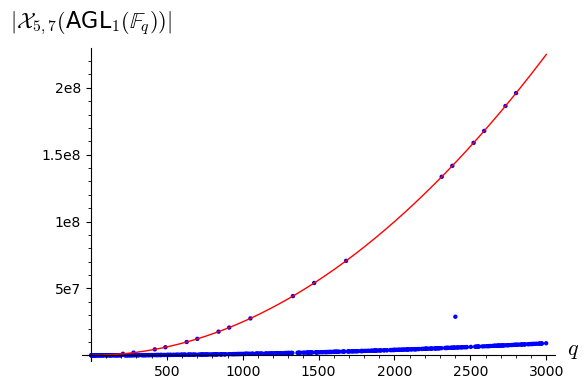
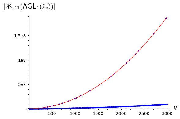
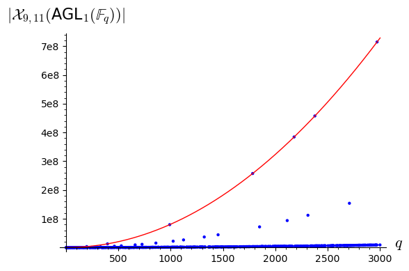
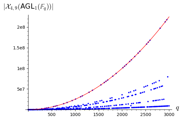
Notice that this erratic behavior poses a philosophical question. Suppose that, for some reason, we know that 𝔛m,n(AGL1())\mathfrak{X}_{m,n}(\mathrm{AGL}_{1}(\mathbb{C})) is polynomial counting. In that case, the degree of the EE-polynomial can be estimated from the dimension of 𝔛m,n(AGL1())\mathfrak{X}_{m,n}(\mathrm{AGL}_{1}(\mathbb{C})). Therefore, an easy way of computing the EE-polynomial is just to start counting points in small finite fields until we get enough interpolating points, which should determine the EE-polynomial. This approach has been used for instance in [9]. However, the previous plot shows that this is not a good idea: most of the prime finite fields give the wrong answer, and only a few (in terms of density) prime powers can be used to interpolate the EE-polynomial.

Moreover, even though we were able to compute the number of points of 𝔛m,n(AGL1(𝔽q))\mathfrak{X}_{m,n}(\mathrm{AGL}_{1}(\mathbb{F}_{q})) for any prime power qq, say through arithmetic arguments, it is not clear how to extract the EE-polynomial from these computations. The computations will only show that the number of points of the variety follows several trends, but the right trend is unknown beforehand (and it is not highlighted by density arguments). The selection rule for the right trend is much deeper and hard to discover: there exists a finitely generated subring of \mathbb{C} that is contained exactly in the finite fields of a single trend. Only one trend can satisfy this property, and that one is the correct trend.

In this spirit, we cannot expect asymptotic polynomial count to be a property that can be read from the motive. However, there is still a hope with strongly polynomial count. This poses the following conjecture which, to our knowledge, is still open.

Conjecture 4.

Let 𝒳\mathcal{X} be a reduced \mathbb{Z}-scheme and let X=𝒳()X=\mathcal{X}(\mathbb{C}) be the associated complex algebraic variety. Then XX is strongly polynomial count if and only if it is polynomial motivic, and the counting and motivic polynomials agree.

6. AGL2(𝐤)\mathrm{AGL}_{2}(\mathbf{k})-representation varieties of torus knots

In this section, we compute the motive of the AGL2(𝐤)\mathrm{AGL}_{2}(\mathbf{k})-representation variety of the (m,n)(m,n)-torus knot. Suppose that we have an element (A,B)𝔛m,n(AGL2(𝐤))(A,B)\in\mathfrak{X}_{m,n}(\mathrm{AGL}_{2}(\mathbf{k})) with matrices of the form

A=(10αA0),B=(10βB0),A=\begin{pmatrix}1&0\\ \alpha&A_{0}\end{pmatrix},\qquad B=\begin{pmatrix}1&0\\ \beta&B_{0}\end{pmatrix},

where A0,B0GL2(𝐤)A_{0},B_{0}\in\mathrm{GL}_{2}(\mathbf{k}) while α,β𝐤2\alpha,\beta\in\mathbf{k}^{2}. Computing the powers we obtain

An=(10Φn(A0)αA0n),Bm=(10Φm(B0)βB0m).A^{n}=\begin{pmatrix}1&0\\ \Phi_{n}(A_{0})\alpha&A^{n}_{0}\end{pmatrix},\qquad B^{m}=\begin{pmatrix}1&0\\ \Phi_{m}(B_{0})\beta&B^{m}_{0}\end{pmatrix}.

Therefore, the AGL2(𝐤)\mathrm{AGL}_{2}(\mathbf{k})-representation variety is explicitly given by

𝔛m,n(AGL2(𝐤))={(A0,B0,α,β)GL2(𝐤)2×𝐤2|A0n=B0mΦn(A0)α=Φm(B0)β}.\mathfrak{X}_{m,n}(\mathrm{AGL}_{2}(\mathbf{k}))=\left\{(A_{0},B_{0},\alpha,\beta)\in\mathrm{GL}_{2}(\mathbf{k})^{2}\times\mathbf{k}^{2}\,\left|\,\begin{matrix}A_{0}^{n}=B_{0}^{m}\\ \Phi_{n}(A_{0})\alpha=\Phi_{m}(B_{0})\beta\end{matrix}\right.\right\}. (4)

In particular, these conditions imply that (A0,B0)𝔛m,n(GL2(𝐤))(A_{0},B_{0})\in\mathfrak{X}_{m,n}(\mathrm{GL}_{2}(\mathbf{k})). Let us decompose the variety as

𝔛m,n(AGL2(𝐤))=𝔛m,nirr(AGL2(𝐤))𝔛m,nred(AGL2(𝐤)).\mathfrak{X}_{m,n}(\mathrm{AGL}_{2}(\mathbf{k}))=\mathfrak{X}_{m,n}^{\mathrm{irr}}(\mathrm{AGL}_{2}(\mathbf{k}))\sqcup\mathfrak{X}_{m,n}^{\mathrm{red}}(\mathrm{AGL}_{2}(\mathbf{k})).

Here, 𝔛m,nirr(AGL2(𝐤))\mathfrak{X}_{m,n}^{\mathrm{irr}}(\mathrm{AGL}_{2}(\mathbf{k})) (resp. 𝔛m,nred(AGL2(𝐤))\mathfrak{X}_{m,n}^{\mathrm{red}}(\mathrm{AGL}_{2}(\mathbf{k}))) are the representations (A,B)(A,B) with (A0,B0)(A_{0},B_{0}) an irreducible (resp. reducible) representation in the algebraic closure 𝐤¯\overline{\mathbf{k}} of 𝐤\mathbf{k}. Note that the superscripts refer to the reducibility/irreducibility of the vectorial part of the representation, not to the representation itself.

First of all, let us analyze the case where (A0,B0)(A_{0},B_{0}) is an irreducible representation. In that case, the eigenvalues are restricted as the following result shows.

Lemma 6.1.

Let ρ=(A0,B0)𝔛m,nirr(GLr(𝐤))\rho=(A_{0},B_{0})\in\mathfrak{X}_{m,n}^{\mathrm{irr}}(\mathrm{GL}_{r}(\mathbf{k})) be an irreducible representation over 𝐤¯\overline{\mathbf{k}}. Then A0n=B0m=ωIdA_{0}^{n}=B_{0}^{m}=\omega\,\mathrm{Id}, for some ω𝐤\omega\in\mathbf{k}^{*}.

Proof.

Notice that A0nA^{n}_{0} is a linear map that is equivariant with respect to the representation ρ\rho. By Schur lemma applied to the algebraic closure 𝐤¯\overline{\mathbf{k}}, this implies that A0nA_{0}^{n} must be a multiple of the identity, say A0n=ωIdA_{0}^{n}=\omega\,\mathrm{Id} for some ω𝐤¯\omega\in\overline{\mathbf{k}} and, since B0m=A0nB_{0}^{m}=A_{0}^{n}, also B0m=ωIdB_{0}^{m}=\omega\,\mathrm{Id}. However, A0nA_{0}^{n} has coefficients in 𝐤\mathbf{k} so ω𝐤\omega\in\mathbf{k}^{*}. ∎

Corollary 6.2.

Let ρ=(A0,B0)𝔛m,nirr(GLr(𝐤))\rho=(A_{0},B_{0})\in\mathfrak{X}_{m,n}^{\mathrm{irr}}(\mathrm{GL}_{r}(\mathbf{k})) be an irreducible representation over 𝐤¯\overline{\mathbf{k}} and let λ1,,λr\lambda_{1},\ldots,\lambda_{r} and η1,,ηr\eta_{1},\ldots,\eta_{r} be the eigenvalues of A0A_{0} and B0B_{0}, respectively. If char(𝐤)\mathrm{char}(\mathbf{k}) does not divide nn and mm, then A0A_{0} and B0B_{0} are diagonalizable and λ1n==λrn=η1m==ηrm\lambda_{1}^{n}=\ldots=\lambda_{r}^{n}=\eta_{1}^{m}=\ldots=\eta_{r}^{m}.

Furthermore, if r=2r=2, char(𝐤)2\mathrm{char}(\mathbf{k})\neq 2, and m,nm,n are odd, then λi,ηj𝐤\lambda_{i},\eta_{j}\in\mathbf{k}^{*}.

Proof.

The first statement is clear since the ll-th power of non-diagonalizable matrix is non-diagonalizable provided that char(𝐤)\mathrm{char}(\mathbf{k}) does not divide ll. For the second, note that λi\lambda_{i} is a root of a polynomial with coefficients in 𝐤\mathbf{k}, so either λi𝐤\lambda_{i}\in\mathbf{k}^{*} or there is a quadratic extension 𝐤𝐤(λi)\mathbf{k}\subset\mathbf{k}(\lambda_{i}). Since 𝐤\mathbf{k} has not characteristic 22, this implies that λi=a+b\lambda_{i}=a+b with a𝐤a\in\mathbf{k} and b2𝐤b^{2}\in\mathbf{k}. Writing n=2r+1n=2r+1 we have that

λin=janibi=j=0ran2jb2j+b(j=0ran2j1b2j).\lambda_{i}^{n}=\sum_{j}a^{n-i}b^{i}=\sum_{j=0}^{r}a^{n-2j}b^{2j}+b\left(\sum_{j=0}^{r}a^{n-2j-1}b^{2j}\right).

Since λin,a,b2j𝐤\lambda_{i}^{n},a,b^{2j}\in\mathbf{k}, it follows that b𝐤b\in\mathbf{k} and thus λi𝐤\lambda_{i}\in\mathbf{k}. ∎

In an analogous way, we have the following result.

Corollary 6.3.

Suppose m,nm,n are odd coprime numbers, char(𝐤)2\mathrm{char}(\mathbf{k})\neq 2, and char(𝐤)\mathrm{char}(\mathbf{k}) does not divide n,mn,m. Let ρ=(A0,B0)𝔛m,nred(GL2(𝐤))\rho=(A_{0},B_{0})\in\mathfrak{X}_{m,n}^{\mathrm{red}}(\mathrm{GL}_{2}(\mathbf{k})) be a reducible representation over 𝐤¯\overline{\mathbf{k}}. Then the eigenvalues λi,ηj𝐤\lambda_{i},\eta_{j}\in\mathbf{k}^{*}, and the eigenvectors are defined over 𝐤\mathbf{k}. In particular, ρ\rho is reducible over 𝐤\mathbf{k}.

Due to the previous results, from now on we shall assume the hypotheses on n,mn,m and char(𝐤)\mathrm{char}(\mathbf{k}) of Corollary 6.3.

6.1. The irreducible stratum

In order to analyze the conditions of (4), observe that (A,B)(A0,B0)(A,B)\mapsto(A_{0},B_{0}) defines a morphism

𝔛m,nirr(AGL2(𝐤))𝔛m,nirr(GL2(𝐤)).\mathfrak{X}_{m,n}^{\mathrm{irr}}(\mathrm{AGL}_{2}(\mathbf{k}))\longrightarrow\mathfrak{X}_{m,n}^{\mathrm{irr}}(\mathrm{GL}_{2}(\mathbf{k})). (5)

The fiber of this morphism at (A0,B0)(A_{0},B_{0}) is the kernel of the map

Λ:𝐤2×𝐤2𝐤2,Λ(α,β)=Φn(A0)αΦm(B0)β.\Lambda:\mathbf{k}^{2}\times\mathbf{k}^{2}\to\mathbf{k}^{2},\quad\Lambda(\alpha,\beta)=\Phi_{n}(A_{0})\alpha-\Phi_{m}(B_{0})\beta. (6)

The following appears in [25, Proposition 7.3] for 𝐤=\mathbf{k}=\mathbb{C}. Recall from Example 2.2 that [PGL2(𝐤)]=q3q[\mathrm{PGL}_{2}(\mathbf{k})]=q^{3}-q.

Proposition 6.4.

For the torus knot of type (m,n)(m,n), with m,nm,n both odd, we have

[𝔛m,nirr(GL2(𝐤))]=14[PGL2(𝐤)]|Ωm,n𝐤|(q2)(q1).[\mathfrak{X}_{m,n}^{\mathrm{irr}}(\mathrm{GL}_{2}(\mathbf{k}))]=\frac{1}{4}[\mathrm{PGL}_{2}(\mathbf{k})]|\Omega_{m,n}^{\mathbf{k}}|(q-2)(q-1).
Proof.

Let (A0,B0)𝔛m,nirr(GL2(𝐤))(A_{0},B_{0})\in\mathfrak{X}_{m,n}^{\mathrm{irr}}(\mathrm{GL}_{2}(\mathbf{k})). Let λ1,λ2\lambda_{1},\lambda_{2} be the eigenvalues of A0A_{0} and η1,η2\eta_{1},\eta_{2} be the eigenvalues of B0B_{0}. Note that λ1n=λ2n=η1m=η2m=ω\lambda_{1}^{n}=\lambda_{2}^{n}=\eta_{1}^{m}=\eta_{2}^{m}=\omega. By Lemma 4.1, we can write λ1=tm\lambda_{1}=t^{m}, η1=tn\eta_{1}=t^{n}, where ω=tnm\omega=t^{nm}, t𝐤t\in\mathbf{k}. Also write λ2=um\lambda_{2}=u^{m}, η2=un\eta_{2}=u^{n}, with ω=unm\omega=u^{nm}. Therefore, u=εtu=\varepsilon t, with εΩm,n𝐤=μnm𝐤(μn𝐤μm𝐤)\varepsilon\in\Omega_{m,n}^{\mathbf{k}}=\mu_{nm}^{\mathbf{k}}-(\mu_{n}^{\mathbf{k}}\cup\mu_{m}^{\mathbf{k}}). This follows since λ1λ2\lambda_{1}\neq\lambda_{2} and η1η2\eta_{1}\neq\eta_{2}, hence εn1\varepsilon^{n}\neq 1, εm1\varepsilon^{m}\neq 1.

Now the ordering of λ1,λ2\lambda_{1},\lambda_{2} and the ordering of η1,η2\eta_{1},\eta_{2} produces an action of 2×2\mathbb{Z}_{2}\times\mathbb{Z}_{2} on Ωn,m𝐤\Omega^{\mathbf{k}}_{n,m}. This action is necessarily free. Therefore the quotient space is given by 14|Ωm,n𝐤|\frac{1}{4}|\Omega_{m,n}^{\mathbf{k}}| elements. For each of them, we have to select points in the space (8) below, hence accounting for q2q-2 and thus the result follows. ∎

To understand the kernel of (6), we use the following lemma.

Lemma 6.5.

Let AA be a diagonalizable matrix and let P(x)[x]P(x)\in\mathbb{C}[x] be a polynomial. Then the dimension of the kernel of the matrix P(A)P(A) is the number of eigenvalues of AA that are roots of P(x)P(x).

Proof.

Write A=QDQ1A=QDQ^{-1} with D=diag(λ1,,λr)D=\textrm{diag}(\lambda_{1},\ldots,\lambda_{r}) a diagonal matrix. Then P(A)=QP(D)Q1P(A)=QP(D)Q^{-1} and, since P(D)=diag(P(λ1),,P(λr))P(D)=\textrm{diag}(P(\lambda_{1}),\ldots,P(\lambda_{r})), the dimension of its kernel is the number of eigenvalues that are also roots of PP. ∎

Recall that we are assuming that the characteristic of 𝐤\mathbf{k} does not divide n,mn,m. Using Lemma 6.5, we get that the dimension of the kernel of Φn(A0)\Phi_{n}(A_{0}) is the number of eigenvalues of A0A_{0} that belong to μ^n𝐤=μn𝐤{1}\hat{\mu}_{n}^{\mathbf{k}}=\mu_{n}^{\mathbf{k}}-\{1\}, and analogously for Φm(B0)\Phi_{m}(B_{0}). Let λ1,λ2\lambda_{1},\lambda_{2} be the eigenvalues of A0A_{0} and η1,η2\eta_{1},\eta_{2} the eigenvalues of B0B_{0}. Recall that λ1λ2\lambda_{1}\neq\lambda_{2} and η1η2\eta_{1}\neq\eta_{2} since otherwise (A0,B0)(A_{0},B_{0}) is not irreducible. Then, we have the following options:

  1. (1)

    Case λ1,λ2μ^n𝐤\lambda_{1},\lambda_{2}\in\hat{\mu}_{n}^{\mathbf{k}} and η1,η2μ^m𝐤\eta_{1},\eta_{2}\in\hat{\mu}_{m}^{\mathbf{k}}. In this situation, Λ0\Lambda\equiv 0 so KerΛ=𝐤4\textrm{Ker}\,{\Lambda}=\mathbf{k}^{4}. Hence, if we denote by 𝔛m,nirr,(1)(AGL2(𝐤))\mathfrak{X}_{m,n}^{\mathrm{irr},(1)}(\mathrm{AGL}_{2}(\mathbf{k})) and 𝔛m,nirr,(1)(GL2(𝐤))\mathfrak{X}_{m,n}^{\mathrm{irr},(1)}(\mathrm{GL}_{2}(\mathbf{k})) the corresponding strata in (5) of the total and base space, respectively, we have that

    [𝔛m,nirr,(1)(AGL2(𝐤))]=[𝔛m,nirr,(1)(GL2(𝐤))][𝐤4].\left[\mathfrak{X}_{m,n}^{\mathrm{irr},(1)}(\mathrm{AGL}_{2}(\mathbf{k}))\right]=\left[\mathfrak{X}_{m,n}^{\mathrm{irr},(1)}(\mathrm{GL}_{2}(\mathbf{k}))\right][\mathbf{k}^{4}].

    To get the motive of 𝔛m,nirr,(1)(GL2(𝐤))\mathfrak{X}_{m,n}^{\mathrm{irr},(1)}(\mathrm{GL}_{2}(\mathbf{k})), the eigenvalues define a fibration

    𝔛m,nirr,(1)(GL2(𝐤))((μ^n𝐤)2Δ)/2×((μ^m𝐤)2Δ)/2,\mathfrak{X}_{m,n}^{\mathrm{irr},(1)}(\mathrm{GL}_{2}(\mathbf{k}))\longrightarrow((\hat{\mu}_{n}^{\mathbf{k}})^{2}-\Delta)/\mathbb{Z}_{2}\times((\hat{\mu}_{m}^{\mathbf{k}})^{2}-\Delta)/\mathbb{Z}_{2}, (7)

    where Δ\Delta is the diagonal and 2\mathbb{Z}_{2} acts by permutation of the entries. The fiber of this map is the collection of representations (A0,B0)𝔛m,nirr(GL2(𝐤))(A_{0},B_{0})\in\mathfrak{X}_{m,n}^{\mathrm{irr}}(\mathrm{GL}_{2}(\mathbf{k})) with fixed eigenvalues, denoted by 𝔛m,nirr(GL2(𝐤))0\mathfrak{X}_{m,n}^{\mathrm{irr}}(\mathrm{GL}_{2}(\mathbf{k}))_{0}. An element of 𝔛m,nirr(GL2(𝐤))0\mathfrak{X}_{m,n}^{\mathrm{irr}}(\mathrm{GL}_{2}(\mathbf{k}))_{0} is completely determined by the two pairs of eigenspaces of (A0,B0)(A_{0},B_{0}) up to conjugation. Since the representation (A0,B0)(A_{0},B_{0}) must be irreducible, these eigenspaces must be pairwise distinct. Hence, this variety is 𝔛m,nirr(GL2(𝐤))0=(𝐤1)4Δc\mathfrak{X}_{m,n}^{\mathrm{irr}}(\mathrm{GL}_{2}(\mathbf{k}))_{0}=(\mathbb{P}_{\mathbf{k}}^{1})^{4}-\Delta_{c}, where Δc(𝐤1)4\Delta_{c}\subset(\mathbb{P}_{\mathbf{k}}^{1})^{4} is the ‘coarse diagonal’ of tuples with two repeated entries. There is a free and closed action of PGL2(𝐤)\mathrm{PGL}_{2}(\mathbf{k}) on (𝐤1)4(\mathbb{P}_{\mathbf{k}}^{1})^{4} with quotient

    (𝐤1)4ΔcPGL2(𝐤)=𝐤1{0,1,}.\frac{(\mathbb{P}_{\mathbf{k}}^{1})^{4}-\Delta_{c}}{\mathrm{PGL}_{2}(\mathbf{k})}=\mathbb{P}_{\mathbf{k}}^{1}-\{0,1,\infty\}. (8)

    To see this, note that there is a PGL2(𝐤)\mathrm{PGL}_{2}(\mathbf{k})-equivariant map that sends the first three entries to 0,1,𝐤10,1,\infty\in\mathbb{P}_{\mathbf{k}}^{1} respectively, so the orbit is completely determined by the image of the fourth point under this map. Hence, [𝔛m,nirr(GL2(𝐤))0]=[𝐤1{0,1,}][PGL2(𝐤)]=(q2)(q3q)[\mathfrak{X}_{m,n}^{\mathrm{irr}}(\mathrm{GL}_{2}(\mathbf{k}))_{0}]=[\mathbb{P}_{\mathbf{k}}^{1}-\{0,1,\infty\}]\,[\mathrm{PGL}_{2}(\mathbf{k})]=(q-2)(q^{3}-q).

    Coming back to the fibration (7), we have that the base space is a set of (ξn𝐤12)(ξm𝐤12)\binom{\xi_{n}^{\mathbf{k}}-1}{2}\binom{\xi_{m}^{\mathbf{k}}-1}{2} points, so

    [𝔛m,nirr,(1)(GL2(𝐤))]=(ξn𝐤1)(ξn𝐤2)(ξm𝐤1)(ξm𝐤2)4(q2)(q3q),\left[\mathfrak{X}_{m,n}^{\mathrm{irr},(1)}(\mathrm{GL}_{2}(\mathbf{k}))\right]=\frac{(\xi^{\mathbf{k}}_{n}-1)(\xi^{\mathbf{k}}_{n}-2)(\xi^{\mathbf{k}}_{m}-1)(\xi^{\mathbf{k}}_{m}-2)}{4}(q-2)(q^{3}-q),

    and thus,

    [𝔛m,nirr,(1)(AGL2(𝐤))]=(ξn𝐤1)(ξn𝐤2)(ξm𝐤1)(ξm𝐤2)4(q52q4)(q3q).\left[\mathfrak{X}_{m,n}^{\mathrm{irr},(1)}(\mathrm{AGL}_{2}(\mathbf{k}))\right]=\frac{(\xi^{\mathbf{k}}_{n}-1)(\xi^{\mathbf{k}}_{n}-2)(\xi^{\mathbf{k}}_{m}-1)(\xi^{\mathbf{k}}_{m}-2)}{4}(q^{5}-2q^{4})(q^{3}-q).
  2. (2)

    Case λ1,λ2μ^n𝐤\lambda_{1},\lambda_{2}\in\hat{\mu}_{n}^{\mathbf{k}}, η1μ^m𝐤\eta_{1}\in\hat{\mu}_{m}^{\mathbf{k}} and η2=1\eta_{2}=1. In this case, KerΛ=𝐤3\textrm{Ker}\,{\Lambda}=\mathbf{k}^{3} and the base space is made of (ξn𝐤12)(m1)\binom{\xi^{\mathbf{k}}_{n}-1}{2}(m-1) copies of 𝔛m,nirr(GL2(𝐤))0\mathfrak{X}_{m,n}^{\mathrm{irr}}(\mathrm{GL}_{2}(\mathbf{k}))_{0}. Hence, this stratum contributes

    [𝔛m,nirr,(2)(AGL2(𝐤))]\displaystyle\left[\mathfrak{X}_{m,n}^{\mathrm{irr},(2)}(\mathrm{AGL}_{2}(\mathbf{k}))\right] =(ξn𝐤1)(ξn𝐤2)(ξm𝐤1)2[1{0,1,}][PGL2(𝐤)][𝐤3]\displaystyle=\frac{(\xi^{\mathbf{k}}_{n}-1)(\xi^{\mathbf{k}}_{n}-2)(\xi^{\mathbf{k}}_{m}-1)}{2}\left[\mathbb{P}^{1}-\left\{0,1,\infty\right\}\right]\,[\mathrm{PGL}_{2}(\mathbf{k})]\,[\mathbf{k}^{3}]
    =(ξn𝐤1)(ξn𝐤2)(ξm𝐤1)2(q42q3)(q3q).\displaystyle=\frac{(\xi^{\mathbf{k}}_{n}-1)(\xi^{\mathbf{k}}_{n}-2)(\xi^{\mathbf{k}}_{m}-1)}{2}(q^{4}-2q^{3})(q^{3}-q).
  3. (3)

    Case λ1μ^n𝐤\lambda_{1}\in\hat{\mu}_{n}^{\mathbf{k}}, λ2=1\lambda_{2}=1 and η1,η2μ^m𝐤\eta_{1},\eta_{2}\in\hat{\mu}_{m}^{\mathbf{k}}. This is analogous to the previous stratum and contributes

    [𝔛m,nirr,(3)(AGL2(𝐤))]\displaystyle\left[\mathfrak{X}_{m,n}^{\mathrm{irr},(3)}(\mathrm{AGL}_{2}(\mathbf{k}))\right] =(ξm𝐤1)(ξn𝐤1)(ξm𝐤2)2[1{0,1,}][PGL2(𝐤)][𝐤3]\displaystyle=\frac{(\xi^{\mathbf{k}}_{m}-1)(\xi^{\mathbf{k}}_{n}-1)(\xi^{\mathbf{k}}_{m}-2)}{2}\left[\mathbb{P}^{1}-\left\{0,1,\infty\right\}\right]\,[\mathrm{PGL}_{2}(\mathbf{k})]\,[\mathbf{k}^{3}]
    =(ξm𝐤1)(ξn𝐤1)(ξm𝐤2)2(q42q3)(q3q).\displaystyle=\frac{(\xi^{\mathbf{k}}_{m}-1)(\xi^{\mathbf{k}}_{n}-1)(\xi^{\mathbf{k}}_{m}-2)}{2}(q^{4}-2q^{3})(q^{3}-q).
  4. (4)

    Case λ1μ^n𝐤\lambda_{1}\in\hat{\mu}_{n}^{\mathbf{k}}, λ2=1\lambda_{2}=1 and η1μ^m𝐤\eta_{1}\in\hat{\mu}_{m}^{\mathbf{k}}, η2=1\eta_{2}=1. Now, KerΛ=𝐤2\textrm{Ker}\,{\Lambda}=\mathbf{k}^{2} and this stratum contributes

    [𝔛m,nirr,(4)(AGL2(𝐤))]\displaystyle\left[\mathfrak{X}_{m,n}^{\mathrm{irr},(4)}(\mathrm{AGL}_{2}(\mathbf{k}))\right] =(ξm𝐤1)(ξn𝐤1)[1{0,1,}][PGL2(𝐤)][𝐤2]\displaystyle=(\xi^{\mathbf{k}}_{m}-1)(\xi^{\mathbf{k}}_{n}-1)\left[\mathbb{P}^{1}-\left\{0,1,\infty\right\}\right]\,[\mathrm{PGL}_{2}(\mathbf{k})]\,[\mathbf{k}^{2}]
    =(ξm𝐤1)(ξn𝐤1)(q32q2)(q3q).\displaystyle=(\xi^{\mathbf{k}}_{m}-1)(\xi^{\mathbf{k}}_{n}-1)(q^{3}-2q^{2})(q^{3}-q).
  5. (5)

    Case λ1μ^n𝐤,λ2μ^n𝐤,η1μ^m𝐤\lambda_{1}\not\in\hat{\mu}_{n}^{\mathbf{k}},\lambda_{2}\not\in\hat{\mu}_{n}^{\mathbf{k}},\eta_{1}\not\in\hat{\mu}_{m}^{\mathbf{k}} and η2μ^m𝐤\eta_{2}\not\in\hat{\mu}_{m}^{\mathbf{k}}. Recall that by Corollary 6.2, these conditions are all equivalent. In this situation, Λ\Lambda is surjective so KerΛ=𝐤2\textrm{Ker}\,{\Lambda}=\mathbf{k}^{2}. The motive [𝔛m,nirr(GL2(𝐤))]\left[\mathfrak{X}_{m,n}^{\mathrm{irr}}(\mathrm{GL}_{2}(\mathbf{k}))\right] is given in Proposition 6.4. To this space, we have to remove the orbits corresponding to the forbidden eigenvalues, which are

    m,n=\displaystyle\ell_{m,n}= (ξn𝐤1)(ξn𝐤2)(ξm𝐤1)(ξm𝐤2)4+(ξn𝐤1)(ξn𝐤2)(ξm𝐤1)2\displaystyle\,\frac{(\xi^{\mathbf{k}}_{n}-1)(\xi^{\mathbf{k}}_{n}-2)(\xi^{\mathbf{k}}_{m}-1)(\xi^{\mathbf{k}}_{m}-2)}{4}+\frac{(\xi^{\mathbf{k}}_{n}-1)(\xi^{\mathbf{k}}_{n}-2)(\xi^{\mathbf{k}}_{m}-1)}{2}
    +(ξm𝐤1)(ξn𝐤1)(ξm𝐤2)2+(ξm𝐤1)(ξn𝐤1)=14ξm𝐤ξn𝐤(ξm𝐤1)(ξn𝐤1)\displaystyle+\frac{(\xi^{\mathbf{k}}_{m}-1)(\xi^{\mathbf{k}}_{n}-1)(\xi^{\mathbf{k}}_{m}-2)}{2}+(\xi^{\mathbf{k}}_{m}-1)(\xi^{\mathbf{k}}_{n}-1)=\frac{1}{4}\xi^{\mathbf{k}}_{m}\xi^{\mathbf{k}}_{n}(\xi^{\mathbf{k}}_{m}-1)(\xi^{\mathbf{k}}_{n}-1)

    copies of [𝔛m,nirr(GL2(𝐤))0]=[1{0,1,}][PGL2(𝐤)][\mathfrak{X}_{m,n}^{\mathrm{irr}}(\mathrm{GL}_{2}(\mathbf{k}))_{0}]=[\mathbb{P}^{1}-\{0,1,\infty\}]\,[\mathrm{PGL}_{2}(\mathbf{k})]. Hence this stratum contributes

    [𝔛m,nirr,(5)(AGL2(𝐤))]=\displaystyle\left[\mathfrak{X}_{m,n}^{\mathrm{irr},(5)}(\mathrm{AGL}_{2}(\mathbf{k}))\right]= ([𝔛m,nirr(GL2(𝐤))]m,n(q2)(q3q))[𝐤2]\displaystyle\left(\left[\mathfrak{X}_{m,n}^{\mathrm{irr}}(\mathrm{GL}_{2}(\mathbf{k}))\right]-\ell_{m,n}(q-2)(q^{3}-q)\right)\left[\mathbf{k}^{2}\right]
    =\displaystyle= [𝔛m,nirr(GL2(𝐤))]q214ξm𝐤ξn𝐤(ξm𝐤1)(ξn𝐤1)(q32q2)(q3q)\displaystyle\left[\mathfrak{X}_{m,n}^{\mathrm{irr}}(\mathrm{GL}_{2}(\mathbf{k}))\right]q^{2}-\frac{1}{4}\xi^{\mathbf{k}}_{m}\xi^{\mathbf{k}}_{n}(\xi^{\mathbf{k}}_{m}-1)(\xi^{\mathbf{k}}_{n}-1)(q^{3}-2q^{2})(q^{3}-q)
    =\displaystyle= 14(q3q)(q32q2)(ξm𝐤1)(ξn𝐤1)(q1ξm𝐤ξn𝐤),\displaystyle\,\frac{1}{4}(q^{3}-q)(q^{3}-2q^{2})(\xi^{\mathbf{k}}_{m}-1)(\xi^{\mathbf{k}}_{n}-1)\big{(}q-1-\xi^{\mathbf{k}}_{m}\xi^{\mathbf{k}}_{n}\big{)},

    using Proposition 6.4 which says that [𝔛m,nirr(GL2(𝐤))]=14(q3q)(ξm𝐤1)(ξn𝐤1)(q2)(q1)[\mathfrak{X}_{m,n}^{\mathrm{irr}}(\mathrm{GL}_{2}(\mathbf{k}))]=\frac{1}{4}(q^{3}-q)(\xi^{\mathbf{k}}_{m}-1)(\xi^{\mathbf{k}}_{n}-1)(q-2)(q-1).

Adding up all the contributions, we get

[𝔛m,nirr(AGL2(𝐤))]=\displaystyle\left[\mathfrak{X}_{m,n}^{\mathrm{irr}}(\mathrm{AGL}_{2}(\mathbf{k}))\right]= [𝔛m,nirr,(1)(AGL2(𝐤))]+[𝔛m,nirr,(2)(AGL2(𝐤))]+[𝔛m,nirr,(3)(AGL2(𝐤))]\displaystyle\left[\mathfrak{X}_{m,n}^{\mathrm{irr},(1)}(\mathrm{AGL}_{2}(\mathbf{k}))\right]+\left[\mathfrak{X}_{m,n}^{\mathrm{irr},(2)}(\mathrm{AGL}_{2}(\mathbf{k}))\right]+\left[\mathfrak{X}_{m,n}^{\mathrm{irr},(3)}(\mathrm{AGL}_{2}(\mathbf{k}))\right]
+[𝔛m,nirr,(4)(AGL2(𝐤))]+[𝔛m,nirr,(5)(AGL2(𝐤))]\displaystyle+\left[\mathfrak{X}_{m,n}^{\mathrm{irr},(4)}(\mathrm{AGL}_{2}(\mathbf{k}))\right]+\left[\mathfrak{X}_{m,n}^{\mathrm{irr},(5)}(\mathrm{AGL}_{2}(\mathbf{k}))\right]
=\displaystyle= (ξm𝐤1)(ξn𝐤1)(q43q3+2q2)(q3q)4((ξm𝐤2)(ξn𝐤2)q+ξm𝐤ξn𝐤3).\displaystyle\,\frac{(\xi^{\mathbf{k}}_{m}-1)(\xi^{\mathbf{k}}_{n}-1)(q^{4}-3q^{3}+2q^{2})(q^{3}-q)}{4}\left((\xi^{\mathbf{k}}_{m}-2)(\xi^{\mathbf{k}}_{n}-2)q+\xi^{\mathbf{k}}_{m}\xi^{\mathbf{k}}_{n}-3\right).

6.2. The reducible stratum

Recall our assumption that char(𝐤)\mathrm{char}(\mathbf{k}) does not divide nn and mm. In this section, we consider the case in which (A0,B0)𝔛m,nred(GL2(𝐤))(A_{0},B_{0})\in\mathfrak{X}_{m,n}^{\mathrm{red}}(\mathrm{GL}_{2}(\mathbf{k})) is a reducible representation. After a change of basis, since A0n=B0mA_{0}^{n}=B_{0}^{m}, we can suppose that (A0,B0)(A_{0},B_{0}) has exactly one of the following three forms:

(A)((t1m00t2m),(t1n00t2n)),(B)((tm00tm),(tn00tn)),(C)((tm0xtm),(tn0ytn)),\textrm{(A)}\left(\begin{pmatrix}t_{1}^{m}&0\\ 0&t_{2}^{m}\end{pmatrix},\begin{pmatrix}t_{1}^{n}&0\\ 0&t_{2}^{n}\end{pmatrix}\right),\textrm{(B)}\left(\begin{pmatrix}t^{m}&0\\ 0&t^{m}\end{pmatrix},\begin{pmatrix}t^{n}&0\\ 0&t^{n}\end{pmatrix}\right),\textrm{(C)}\left(\begin{pmatrix}t^{m}&0\\ x&t^{m}\end{pmatrix},\begin{pmatrix}t^{n}&0\\ y&t^{n}\end{pmatrix}\right),

with t1,t2,t𝐤t_{1},t_{2},t\in\mathbf{k}^{*}, x,y𝐤x,y\in\mathbf{k} and satisfying t1t2t_{1}\neq t_{2} and (x,y)(0,0)(x,y)\neq(0,0).

Restricting to the representations of each stratum S=(A),(B),(C)S=(\textrm{A}),(\textrm{B}),(\textrm{C}), we have a morphism

𝔛m,nS(AGL2(𝐤))𝔛m,nS(GL2(𝐤)),\mathfrak{X}_{m,n}^{S}(\mathrm{AGL}_{2}(\mathbf{k}))\longrightarrow\mathfrak{X}_{m,n}^{S}(\mathrm{GL}_{2}(\mathbf{k})), (9)

whose fiber is the kernel of the linear map (6).

6.2.1. Case (A)

In this case, as for the irreducible part of Section 6.1, the kernel of Λ\Lambda depends on whether t1,t2t_{1},t_{2} are roots of the polynomial Φl\Phi_{l}. In this case the base space is

𝔛m,n(A)(GL2(𝐤))=(((𝐤)2Δ)×GL2(𝐤)GL1(𝐤)×GL1(𝐤))/2,\mathfrak{X}_{m,n}^{\textrm{(A)}}(\mathrm{GL}_{2}(\mathbf{k}))=\left(\left((\mathbf{k}^{*})^{2}-\Delta\right)\times\frac{\mathrm{GL}_{2}(\mathbf{k})}{\mathrm{GL}_{1}(\mathbf{k})\times\mathrm{GL}_{1}(\mathbf{k})}\right)/\mathbb{Z}_{2},

with the action of 2\mathbb{Z}_{2} given by exchange of eigenvalues and eigenvectors. Using Lemma 2.3 and (1), we have

[𝔛m,n(A)(GL2(𝐤))]\displaystyle\left[\mathfrak{X}_{m,n}^{\mathrm{(A)}}(\mathrm{GL}_{2}(\mathbf{k}))\right] =[(𝐤)2Δ]+[GL2(𝐤)GL1(𝐤)×GL1(𝐤)]++[(𝐤)2Δ][GL2(𝐤)GL1(𝐤)×GL1(𝐤)]\displaystyle=[(\mathbf{k}^{*})^{2}-\Delta]^{+}\left[\frac{\mathrm{GL}_{2}(\mathbf{k})}{\mathrm{GL}_{1}(\mathbf{k})\times\mathrm{GL}_{1}(\mathbf{k})}\right]^{+}+[(\mathbf{k}^{*})^{2}-\Delta]^{-}\left[\frac{\mathrm{GL}_{2}(\mathbf{k})}{\mathrm{GL}_{1}(\mathbf{k})\times\mathrm{GL}_{1}(\mathbf{k})}\right]^{-}
=q2(q1)2q(q1).\displaystyle=q^{2}(q-1)^{2}-q(q-1).

On the other hand, if we fix the eigenvalues of (A0,B0)(A_{0},B_{0}) as in Section 6.1, the corresponding fiber 𝔛m,n(A)(GL2(𝐤))0\mathfrak{X}_{m,n}^{\mathrm{(A)}}(\mathrm{GL}_{2}(\mathbf{k}))_{0} is

[𝔛m,n(A)(GL2(𝐤))0]=[GL2(𝐤)GL1(𝐤)×GL1(𝐤)]=q2+q.\left[\mathfrak{X}_{m,n}^{\mathrm{(A)}}(\mathrm{GL}_{2}(\mathbf{k}))_{0}\right]=\left[\frac{\mathrm{GL}_{2}(\mathbf{k})}{\mathrm{GL}_{1}(\mathbf{k})\times\mathrm{GL}_{1}(\mathbf{k})}\right]=q^{2}+q.

As in Section 4, set Ωm,n𝐤=μmn𝐤(μm𝐤μn𝐤)\Omega^{\mathbf{k}}_{m,n}=\mu_{mn}^{\mathbf{k}}-(\mu_{m}^{\mathbf{k}}\cup\mu_{n}^{\mathbf{k}}) for those t𝐤t\in\mathbf{k}^{*} such that Φn(tm)=0\Phi_{n}(t^{m})=0 and Φm(tn)=0\Phi_{m}(t^{n})=0. With this information at hand, we compute for each stratum:

  1. (1)

    Case t1,t2Ωm,n𝐤t_{1},t_{2}\in\Omega^{\mathbf{k}}_{m,n}. In this situation, Λ0\Lambda\equiv 0 so KerΛ=𝐤4\textrm{Ker}\,{\Lambda}=\mathbf{k}^{4}. The eigenvalues yield a fibration

    𝔛m,n(A),(1)(GL2(𝐤))((Ωm,n𝐤)2Δ)/2\mathfrak{X}_{m,n}^{\mathrm{(A)},(1)}(\mathrm{GL}_{2}(\mathbf{k}))\longrightarrow\left((\Omega_{m,n}^{\mathbf{k}})^{2}-\Delta\right)/\mathbb{Z}_{2}

    whose fiber is 𝔛m,n(A)(GL2(𝐤))0\mathfrak{X}_{m,n}^{\mathrm{(A)}}(\mathrm{GL}_{2}(\mathbf{k}))_{0}. Observe that ((Ωm,n𝐤)2Δ)/2\left((\Omega_{m,n}^{\mathbf{k}})^{2}-\Delta\right)/\mathbb{Z}_{2} is a finite set of (ξm𝐤1)(ξn𝐤1)((ξm𝐤1)(ξn𝐤1)1)/2(\xi^{\mathbf{k}}_{m}-1)(\xi^{\mathbf{k}}_{n}-1)((\xi^{\mathbf{k}}_{m}-1)(\xi^{\mathbf{k}}_{n}-1)-1)/2 points, so we have

    [𝔛m,n(A),(1)(AGL2(𝐤))]\displaystyle\left[\mathfrak{X}_{m,n}^{\mathrm{(A)},(1)}(\mathrm{AGL}_{2}(\mathbf{k}))\right] =[𝔛m,n(A),(1)(GL2(𝐤))][𝐤4]\displaystyle=\left[\mathfrak{X}_{m,n}^{\mathrm{(A)},(1)}(\mathrm{GL}_{2}(\mathbf{k}))\right][\mathbf{k}^{4}]
    =[𝔛m,n(A)(GL2(𝐤))0][𝐤4][((Ωm,n𝐤)2Δ)/2]\displaystyle=\left[\mathfrak{X}_{m,n}^{\mathrm{(A)}}(\mathrm{GL}_{2}(\mathbf{k}))_{0}\right][\mathbf{k}^{4}]\left[\left((\Omega_{m,n}^{\mathbf{k}})^{2}-\Delta\right)/\mathbb{Z}_{2}\right]
    =(ξm𝐤1)(ξn𝐤1)(ξm𝐤ξn𝐤ξm𝐤ξn𝐤)2q4(q2+q).\displaystyle=\frac{(\xi^{\mathbf{k}}_{m}-1)(\xi^{\mathbf{k}}_{n}-1)(\xi^{\mathbf{k}}_{m}\xi^{\mathbf{k}}_{n}-\xi^{\mathbf{k}}_{m}-\xi^{\mathbf{k}}_{n})}{2}q^{4}(q^{2}+q).
  2. (2)

    Case t1Ωm,n𝐤t_{1}\in\Omega^{\mathbf{k}}_{m,n} but t2Ωm,n𝐤t_{2}\not\in\Omega^{\mathbf{k}}_{m,n} (or vice-versa, the order is not important here). Now, we have a locally trivial fibration

    𝔛m,n(A),(2)(GL2(𝐤))Ωm,n𝐤×(𝐤Ωm,n𝐤),\mathfrak{X}_{m,n}^{\mathrm{(A)},(2)}(\mathrm{GL}_{2}(\mathbf{k}))\longrightarrow\Omega^{\mathbf{k}}_{m,n}\times\left(\mathbf{k}^{*}-\Omega^{\mathbf{k}}_{m,n}\right),

    with fiber 𝔛m,n(A)(GL2(𝐤))0\mathfrak{X}_{m,n}^{\mathrm{(A)}}(\mathrm{GL}_{2}(\mathbf{k}))_{0}. The kernel of Λ\Lambda is 𝐤3\mathbf{k}^{3}, so this stratum contributes

    [𝔛m,n(A),(2)(AGL2(𝐤))]=(ξm𝐤1)(ξn𝐤1)(qξm𝐤ξn𝐤+ξm𝐤+ξn𝐤2)q3(q2+q).\displaystyle\left[\mathfrak{X}_{m,n}^{\mathrm{(A)},(2)}(\mathrm{AGL}_{2}(\mathbf{k}))\right]=(\xi^{\mathbf{k}}_{m}-1)(\xi^{\mathbf{k}}_{n}-1)(q-\xi^{\mathbf{k}}_{m}\xi^{\mathbf{k}}_{n}+\xi^{\mathbf{k}}_{m}+\xi^{\mathbf{k}}_{n}-2)q^{3}(q^{2}+q).
  3. (3)

    Case t1,t2Ωm,n𝐤t_{1},t_{2}\not\in\Omega^{\mathbf{k}}_{m,n}. The kernel is now 𝐤2\mathbf{k}^{2} and we have a fibration

    𝔛m,n(A),(3)(GL2(𝐤))B,\mathfrak{X}_{m,n}^{\mathrm{(A)},(3)}(\mathrm{GL}_{2}(\mathbf{k}))\longrightarrow B,

    where the motive of the base space BB is

    [B]\displaystyle[B] =[(𝐤)2Δ]+[(Ωm,n𝐤)2Δ]+[Ωm,n𝐤](q1[Ωm,n𝐤])=\displaystyle=[(\mathbf{k}^{*})^{2}-\Delta]^{+}-\left[(\Omega_{m,n}^{\mathbf{k}})^{2}-\Delta\right]^{+}-\left[\Omega^{\mathbf{k}}_{m,n}\right]\left(q-1-[\Omega^{\mathbf{k}}_{m,n}]\right)=
    =(q1)2(ξm𝐤1)(ξn𝐤1)(ξm𝐤ξn𝐤ξm𝐤ξn𝐤)2\displaystyle=(q-1)^{2}-\frac{(\xi^{\mathbf{k}}_{m}-1)(\xi^{\mathbf{k}}_{n}-1)(\xi^{\mathbf{k}}_{m}\xi^{\mathbf{k}}_{n}-\xi^{\mathbf{k}}_{m}-\xi^{\mathbf{k}}_{n})}{2}
    (ξm𝐤1)(ξn𝐤1)(qξm𝐤ξn𝐤+ξm𝐤+ξn𝐤2)\displaystyle\;\;\;\;-(\xi^{\mathbf{k}}_{m}-1)(\xi^{\mathbf{k}}_{n}-1)(q-\xi^{\mathbf{k}}_{m}\xi^{\mathbf{k}}_{n}+\xi^{\mathbf{k}}_{m}+\xi^{\mathbf{k}}_{n}-2)
    =q2(ξm𝐤ξn𝐤ξm𝐤ξn𝐤+3)q14(ξm𝐤1)(ξn𝐤1)(ξm𝐤ξn𝐤8).\displaystyle=q^{2}-(\xi^{\mathbf{k}}_{m}\xi^{\mathbf{k}}_{n}-\xi^{\mathbf{k}}_{m}-\xi^{\mathbf{k}}_{n}+3)q-\frac{1}{4}(\xi^{\mathbf{k}}_{m}-1)(\xi^{\mathbf{k}}_{n}-1)(\xi^{\mathbf{k}}_{m}\xi^{\mathbf{k}}_{n}-8).

    Therefore, this space contributes

    [𝔛m,n(A),(3)\displaystyle\big{[}\mathfrak{X}_{m,n}^{\mathrm{(A)},(3)} (AGL2(𝐤))]=[𝔛m,n(A),(3)(GL2(𝐤))][𝐤2]\displaystyle(\mathrm{AGL}_{2}(\mathbf{k}))\big{]}=\left[\mathfrak{X}_{m,n}^{\mathrm{(A)},(3)}(\mathrm{GL}_{2}(\mathbf{k}))\right][\mathbf{k}^{2}]
    =q2(q2+q)(q2(ξm𝐤ξn𝐤ξm𝐤ξn𝐤+3)q+14(ξm𝐤1)(ξn𝐤1)(ξm𝐤ξn𝐤8)).\displaystyle=q^{2}(q^{2}+q)\left(q^{2}-(\xi^{\mathbf{k}}_{m}\xi^{\mathbf{k}}_{n}-\xi^{\mathbf{k}}_{m}-\xi^{\mathbf{k}}_{n}+3)q+\frac{1}{4}(\xi^{\mathbf{k}}_{m}-1)(\xi^{\mathbf{k}}_{n}-1)(\xi^{\mathbf{k}}_{m}\xi^{\mathbf{k}}_{n}-8)\right).

Adding up all the contributions, we get that

[𝔛m,n(A)(AGL2(𝐤))]=\displaystyle\left[\mathfrak{X}_{m,n}^{\mathrm{(A)}}(\mathrm{AGL}_{2}(\mathbf{k}))\right]=\; (q2+q)q2(12(ξm𝐤1)(ξn𝐤1)(ξm𝐤ξn𝐤ξm𝐤ξn𝐤)(q21)\displaystyle(q^{2}+q)q^{2}\bigg{(}\frac{1}{2}(\xi^{\mathbf{k}}_{m}-1)(\xi^{\mathbf{k}}_{n}-1)(\xi^{\mathbf{k}}_{m}\xi^{\mathbf{k}}_{n}-\xi^{\mathbf{k}}_{m}-\xi^{\mathbf{k}}_{n})(q^{2}-1)
+(ξm𝐤1)(ξn𝐤1)(qξm𝐤ξn𝐤+ξm𝐤+ξn𝐤2)(q1)+(q1)2).\displaystyle+(\xi^{\mathbf{k}}_{m}-1)(\xi^{\mathbf{k}}_{n}-1)(q-\xi^{\mathbf{k}}_{m}\xi^{\mathbf{k}}_{n}+\xi^{\mathbf{k}}_{m}+\xi^{\mathbf{k}}_{n}-2)(q-1)+(q-1)^{2}\bigg{)}.

6.2.2. Case (B)

In this setting, this situation is simpler. Observe that the adjoint action of GL2(𝐤)\mathrm{GL}_{2}(\mathbf{k}) on the vectorial part is trivial, so the corresponding GL2(𝐤)\mathrm{GL}_{2}(\mathbf{k})-representation variety is just

𝔛m,n(B)(GL2(𝐤))=𝐤.\mathfrak{X}_{m,n}^{\mathrm{(B)}}(\mathrm{GL}_{2}(\mathbf{k}))=\mathbf{k}^{*}.

Analogously, the variety with fixed eigenvalues, 𝔛m,n(B)(GL2(𝐤))0\mathfrak{X}_{m,n}^{\mathrm{(B)}}(\mathrm{GL}_{2}(\mathbf{k}))_{0}, is just a point. With these observations, we obtain that:

  1. (1)

    If tΩm,n𝐤t\in\Omega^{\mathbf{k}}_{m,n}, then KerΛ=𝐤4\textrm{Ker}\,{\Lambda}=\mathbf{k}^{4}. We have a fibration

    𝔛m,n(B),(1)(GL2(𝐤))Ωm,n𝐤\mathfrak{X}_{m,n}^{\mathrm{(B)},(1)}(\mathrm{GL}_{2}(\mathbf{k}))\longrightarrow\Omega^{\mathbf{k}}_{m,n}

    whose fiber is 𝔛m,n(B)(GL2(𝐤))0\mathfrak{X}_{m,n}^{\mathrm{(B)}}(\mathrm{GL}_{2}(\mathbf{k}))_{0}. Hence, this stratum contributes

    [𝔛m,n(B),(1)(AGL2(𝐤))]=[𝔛m,n(B),(1)(GL2(𝐤))][𝐤4]=(ξm𝐤1)(ξn𝐤1)q4.\left[\mathfrak{X}_{m,n}^{\mathrm{(B)},(1)}(\mathrm{AGL}_{2}(\mathbf{k}))\right]=\left[\mathfrak{X}_{m,n}^{\mathrm{(B)},(1)}(\mathrm{GL}_{2}(\mathbf{k}))\right][\mathbf{k}^{4}]=(\xi^{\mathbf{k}}_{m}-1)(\xi^{\mathbf{k}}_{n}-1)q^{4}\,.
  2. (2)

    If tΩm,n𝐤t\not\in\Omega^{\mathbf{k}}_{m,n}, then KerΛ=𝐤2\textrm{Ker}\,{\Lambda}=\mathbf{k}^{2}. We have a fibration

    𝔛m,n(B),(2)(GL2(𝐤))𝐤Ωm,n𝐤.\mathfrak{X}_{m,n}^{\mathrm{(B)},(2)}(\mathrm{GL}_{2}(\mathbf{k}))\longrightarrow\mathbf{k}^{*}-\Omega^{\mathbf{k}}_{m,n}.

    Thus, the contribution of this stratum is

    [𝔛m,n(B),(2)(AGL2(𝐤))]=(q1(ξm𝐤1)(ξn𝐤1))q2.\left[\mathfrak{X}_{m,n}^{\mathrm{(B)},(2)}(\mathrm{AGL}_{2}(\mathbf{k}))\right]=(q-1-(\xi^{\mathbf{k}}_{m}-1)(\xi^{\mathbf{k}}_{n}-1))q^{2}.

The total contribution is thus

[𝔛m,n(B)(AGL2(𝐤))]=(ξm𝐤1)(ξn𝐤1)(q4q2)+(q1)q2.\left[\mathfrak{X}_{m,n}^{\mathrm{(B)}}(\mathrm{AGL}_{2}(\mathbf{k}))\right]=(\xi^{\mathbf{k}}_{m}-1)(\xi^{\mathbf{k}}_{n}-1)(q^{4}-q^{2})+(q-1)q^{2}.

6.2.3. Case (C)

In this case, an extra calculation must be done to control the off-diagonal entry. If (A0,B0)(A_{0},B_{0}) has the form

((tm0xtm),(tn0ytn)),\left(\begin{pmatrix}t^{m}&0\\ x&t^{m}\end{pmatrix},\begin{pmatrix}t^{n}&0\\ y&t^{n}\end{pmatrix}\right),

then the condition A0n=B0mA_{0}^{n}=B_{0}^{m} reads as

(tmn0ntm(n1)xtmn)=(tmn0mtn(m1)ytmn).\begin{pmatrix}t^{mn}&0\\ nt^{m(n-1)}x&t^{mn}\end{pmatrix}=\begin{pmatrix}t^{mn}&0\\ mt^{n(m-1)}y&t^{mn}\end{pmatrix}.

The later conditions reduce to ntm(n1)x=mtn(m1)ynt^{m(n-1)}x=mt^{n(m-1)}y and, since t0t\neq 0, this means that (x,y)(x,y) should lie in a line minus (0,0)(0,0). The stabilizer of a Jordan type matrix in GL2(𝐤)\mathrm{GL}_{2}(\mathbf{k}) is the subgroup U=(𝐤)2×𝐤GL2(𝐤)U=(\mathbf{k}^{*})^{2}\times\mathbf{k}\subset\mathrm{GL}_{2}(\mathbf{k}) of upper triangular matrices. Hence, the corresponding GL2(𝐤)\mathrm{GL}_{2}(\mathbf{k})-representation variety is

𝔛m,n(C)(GL2(𝐤))=(𝐤)2×GL2(𝐤)/U.\mathfrak{X}_{m,n}^{\mathrm{(C)}}(\mathrm{GL}_{2}(\mathbf{k}))=(\mathbf{k}^{*})^{2}\times\mathrm{GL}_{2}(\mathbf{k})/U.

In particular, [𝔛m,n(C)(GL2(𝐤))]=(q1)2(q4q3q2+q)/q(q1)2=(q1)2(q+1)\left[\mathfrak{X}_{m,n}^{\mathrm{(C)}}(\mathrm{GL}_{2}(\mathbf{k}))\right]=(q-1)^{2}(q^{4}-q^{3}-q^{2}+q)/q(q-1)^{2}=(q-1)^{2}(q+1). Moreover, if we fix the eigenvalues we get that [𝔛m,n(C)(GL2(𝐤))0]=[𝐤×GL2(𝐤)/U]=(q1)(q+1)\left[\mathfrak{X}_{m,n}^{\mathrm{(C)}}(\mathrm{GL}_{2}(\mathbf{k}))_{0}\right]=\left[\mathbf{k}^{*}\times\mathrm{GL}_{2}(\mathbf{k})/U\right]=(q-1)(q+1).

To analyze the condition Φn(A0)=Φm(B0)\Phi_{n}(A_{0})=\Phi_{m}(B_{0}), a straightforward computation reduces it to

(Φn(tm)0xi=1n1itm(i1)Φn(tm))=(Φm(tn)0yi=1m1itn(i1)Φm(tn)).\begin{pmatrix}\Phi_{n}(t^{m})&0\\ \displaystyle{x\sum_{i=1}^{n-1}it^{m(i-1)}}&\Phi_{n}(t^{m})\end{pmatrix}=\begin{pmatrix}\Phi_{m}(t^{n})&0\\ \displaystyle{y\sum_{i=1}^{m-1}it^{n(i-1)}}&\Phi_{m}(t^{n})\end{pmatrix}.

The off-diagonal entries can be recognized as xΦn(tm)x\Phi_{n}^{\prime}(t^{m}) and yΦm(tn)y\Phi_{m}^{\prime}(t^{n}) respectively, where Φl(x)\Phi_{l}^{\prime}(x) denotes the formal derivative of Φl(x)\Phi_{l}(x). Observe that Φl(x)(x1)=xl1\Phi_{l}(x)(x-1)=x^{l}-1, whose derivative is lxl1lx^{l-1}, so Φl\Phi_{l} has no repeated roots provided that char(𝐤)\mathrm{char}(\mathbf{k}) does not divide ll. Hence, with our assumptions on char(𝐤)\mathrm{char}(\mathbf{k}) we have that Φn(tm),Φm(tn),Φn(tm)\Phi_{n}(t^{m}),\Phi_{m}(t^{n}),\Phi_{n}^{\prime}(t^{m}) and Φm(tn)\Phi_{m}^{\prime}(t^{n}) cannot vanish simultaneously. Therefore, stratifying according to the kernel of Λ\Lambda we get the following two possibilities:

  1. (1)

    If tΩm,n𝐤t\in\Omega^{\mathbf{k}}_{m,n}, then KerΛ=𝐤3\textrm{Ker}\,{\Lambda}=\mathbf{k}^{3}. We have a fibration

    𝔛m,n(C),(1)(GL2(𝐤))Ωm,n𝐤\mathfrak{X}_{m,n}^{\mathrm{(C)},(1)}(\mathrm{GL}_{2}(\mathbf{k}))\longrightarrow\Omega^{\mathbf{k}}_{m,n}

    whose fiber is 𝔛m,n(C)(GL2(𝐤))0\mathfrak{X}_{m,n}^{\mathrm{(C)}}(\mathrm{GL}_{2}(\mathbf{k}))_{0}. Hence, this stratum contributes

    [𝔛m,n(C),(1)(AGL2(𝐤))]=[𝔛m,n(C),(1)(GL2(𝐤))][𝐤3]=(ξm𝐤1)(ξn𝐤1)q3(q1)(q+1).\left[\mathfrak{X}_{m,n}^{\mathrm{(C)},(1)}(\mathrm{AGL}_{2}(\mathbf{k}))\right]=\left[\mathfrak{X}_{m,n}^{\mathrm{(C)},(1)}(\mathrm{GL}_{2}(\mathbf{k}))\right][\mathbf{k}^{3}]=(\xi^{\mathbf{k}}_{m}-1)(\xi^{\mathbf{k}}_{n}-1)q^{3}(q-1)(q+1).
  2. (2)

    If t𝐤Ωm,n𝐤t\in\mathbf{k}^{*}-\Omega^{\mathbf{k}}_{m,n}, then KerΛ=𝐤2\textrm{Ker}\,{\Lambda}=\mathbf{k}^{2}. The fibration we get is now

    𝔛m,n(C),(2)(GL2(𝐤))𝐤Ωm,n𝐤.\mathfrak{X}_{m,n}^{\mathrm{(C)},(2)}(\mathrm{GL}_{2}(\mathbf{k}))\longrightarrow\mathbf{k}^{*}-\Omega^{\mathbf{k}}_{m,n}\,.

    Therefore, this stratum contributes

    [𝔛m,n(C),(2)(AGL2(𝐤))]\displaystyle\left[\mathfrak{X}_{m,n}^{\mathrm{(C)},(2)}(\mathrm{AGL}_{2}(\mathbf{k}))\right] =[𝔛m,n(C),(2)(GL2(𝐤))][𝐤2]\displaystyle=\left[\mathfrak{X}_{m,n}^{\mathrm{(C)},(2)}(\mathrm{GL}_{2}(\mathbf{k}))\right][\mathbf{k}^{2}]
    =[𝔛m,n(C)(GL2(𝐤))(ξm𝐤1)(ξn𝐤1)𝔛m,n(C),(2)(GL2(𝐤))0][𝐤2]\displaystyle=\left[\mathfrak{X}_{m,n}^{\mathrm{(C)}}(\mathrm{GL}_{2}(\mathbf{k}))-(\xi^{\mathbf{k}}_{m}-1)(\xi^{\mathbf{k}}_{n}-1)\mathfrak{X}_{m,n}^{\mathrm{(C)},(2)}(\mathrm{GL}_{2}(\mathbf{k}))_{0}\right][\mathbf{k}^{2}]
    =((q1)2(q+1)(ξm𝐤1)(ξn𝐤1)(q1)(q+1))q2.\displaystyle=\left((q-1)^{2}(q+1)-(\xi^{\mathbf{k}}_{m}-1)(\xi^{\mathbf{k}}_{n}-1)(q-1)(q+1)\right)q^{2}.

Adding up all the contributions, we get that

[𝔛m,n(C)(AGL2(𝐤))]=(q1)2(q+1)q2+(ξm𝐤1)(ξn𝐤1)(q1)(q+1)(q3q2).\left[\mathfrak{X}_{m,n}^{\mathrm{(C)}}(\mathrm{AGL}_{2}(\mathbf{k}))\right]=(q-1)^{2}(q+1)q^{2}+(\xi^{\mathbf{k}}_{m}-1)(\xi^{\mathbf{k}}_{n}-1)(q-1)(q+1)(q^{3}-q^{2}).

Putting the results of Sections 6.1, 6.2.1, 6.2.2 and 6.2.3 together, we prove the second formula in Theorem 1.1.

References

  • [1] D. Baraglia and P. Hekmati, Arithmetic of singular character varieties and their EE-polynomials, Proc. Lond. Math. Soc. (3), 114 (2017), 293–332.
  • [2] L.A. Borisov, The class of the affine line is a zero divisor in the Grothendieck ring, J. Algebraic Geom. 27 (2018), 203–209.
  • [3] M. Culler, P.B. Shalen, Varieties of group representations and splitting of 33-manifolds, Ann. of Math. (2) 117, 109–146, (1983).
  • [4] P. Deligne, Théorie de Hodge II, Publ. Math. I.H.E.S. 40, 5–58, (1971).
  • [5] P. Deligne, Théorie de Hodge III, Publ. Math. I.H.E.S. 44, 5–77, (1974).
  • [6] Á. González-Prieto, Pseudo-quotients of algebraic actions and their application to character varieties, arxiv.org/abs/1807.08540v4.
  • [7] Á. González-Prieto, Motivic theory of representation varieties via Topological Quantum Field Theories, arxiv.org/abs/1810.09714v2.
  • [8] Á. González-Prieto, M. Logares, V. Muñoz, A lax monoidal Topological Quantum Field Theory for representation varieties, Bulletin des Sciences Mathématiques, to appear.
  • [9] Á. González-Prieto, M. Logares, V. Muñoz, Representation variety for the rank one affine group. In eds.  I.N. Parasidis, E. Providas and Th.M. Rassias, Mathematical Analysis in Interdisciplinary Research, Springer, to appear.
  • [10] Á. González-Prieto, M. Logares, V. Muñoz, Motive of the representation varieties of torus knots for low rank affine groups. In eds. P. Pardalos and Th.M. Rassias, Analysis, Geometry, Nonlinear Optimization and Applications, World Scientific Publ. Co., to appear.
  • [11] Á. González-Prieto, V. Muñoz, Motive of the SL4\mathrm{SL}_{4}-character variety of torus knots, arxiv.org/abs/2006.01810
  • [12] T. Hausel, E. Letelier, F.R. Villegas, Arithmetic harmonic analysis on character and quiver varieties II, Advances in Math., 234, 85–128, (2013).
  • [13] T. Hausel and F. Rodríguez-Villegas, Mixed Hodge polynomials of character varieties. With an appendix by Nicholas M. Katz, Invent. Math. 174 (2008) 555–624.
  • [14] T. Hausel, M. Thaddeus, Mirror symmetry, Langlands duality, and the Hitchin system, Invent. Math. 153, 197–229, (2003).
  • [15] N.J. Hitchin, The self-duality equations on a Riemann surface, Proc. London Math. Soc. (3) 55, 59–126, (1987).
  • [16] S. Lawton, V. Muñoz, E-polynomial of the SL(3,)\mathrm{SL}(3,\mathbb{C})-character variety of free groups, Pacific J. Math. 282, 173–202, (2016).
  • [17] M. Logares, V. Muñoz, P.E. Newstead, Hodge polynomials of SL(2,)\mathrm{SL}(2,\mathbb{C})-character varieties for curves of small genus, Rev. Mat. Complut. 26, 635–703, (2013).
  • [18] A. Lubotzky, A.R. Magid, Varieties of representations of finitely generated groups, Mem. Amer. Math. Soc. 58 (1985).
  • [19] J Martín-Morales, A M Oller-Marcén, Combinatorial aspects of the character variety of a family of one-relator groups, Topology Appl. 156, 2376–2389, (2009).
  • [20] J. Martínez, E-polynomials of PGL(2,)\mathrm{PGL}(2,\mathbb{C})-character varieties of surface groups, arxiv.org/abs/1705.04649.
  • [21] J. Martínez, V. Muñoz, E-polynomials of the SL(2,)\mathrm{SL}(2,\mathbb{C})-character varieties of surface groups, Internat. Math. Research Notices 2016, 926–961, (2016).
  • [22] J. Martínez, V. Muñoz, E-polynomial of the SL(2,)\mathrm{SL}(2,\mathbb{C})-character variety of a complex curve of genus 33, Osaka J. Math. 53, 645–681, (2016).
  • [23] M. Mereb, On the EE-polynomials of a family of SLn{\rm SL}_{n}-character varieties, Math. Ann., 363 (2015), 857–892.
  • [24] V. Muñoz, The SL(2,)\mathrm{SL}(2,\mathbb{C})-character varieties of torus knots, Rev. Mat. Complut. 22, 489–497, (2009).
  • [25] V. Muñoz, J. Porti, Geometry of the SL(3,)\mathrm{SL}(3,\mathbb{C})-character variety of torus knots, Algebraic and Geometric Topology 16, 397–426, (2016).
  • [26] M. Nagata, Invariants of a group in an affine ring, J. Math. Kyoto Univ. 3, 369–377, (1963/1964).
  • [27] P. E. Newstead, Introduction to moduli problems and orbit spaces, Tata Institute of Fundamental Research Lectures on Mathematics and Physics 51, (TIFR, 1978).
  • [28] D. Rolfsen, Knots and links, Mathematics Lecture Series 7, (Publish or Perish, 1990).