The Plasma-prescribed Active Region Static Extrapolation (PARSE) Dataset: A Machine-Learning-Ready Collection of Magnetohydrostatic Coronal Active Regions
Abstract
As Physics-Informed Neural Networks and other methods for full-vector-field construction or analysis become more prominent, a need has developed for a large set of simulated active regions for training, validation and testing purposes. We use a state-of-the-art magnetohydrostatic extrapolation method to develop a public dataset of over five thousand data cubes based on the Spaceweather HMI Active Region Patch (SHARP) library of active region magnetogram images. Each cube resolves the magnetic field vector and plasma forcing at approximately 100,000 scattered points that are adaptively clustered near the high-flux regions of the domain. This paper describes the methodology of construction of the Plasma-prescribed Active Region Static Extrapolation (PARSE) dataset, as well as its structure and how to access it.
1 Introduction
The Plasma-prescribed Active Region Static Extrapolation (PARSE) dataset consists of nearly-magnetohydrostatic (MHS), low-divergence extrapolations of photospheric boundary conditions. These boundary conditions are sourced from the Space weather HMI Active Region Patch (SHARP) image pipeline for the Helioseismic and Magnetic Imager (HMI) (Bobra et al., 2014), and represent actual active regions which were present on the sun. Some of these active regions emitted flares or coronal mass ejections during their life cycle, and as such may encode interesting information in the volumetric magnetic vector field. By providing several possible magnetic configurations for each active region, we hope to facilitate a broad range of scientific pursuits. The varying structure and large quantity of the solutions may allow for the use of the dataset to train or validate physics-informed neural networks.
The extrapolation is performed by the Radial-Basis-Function Finite-Difference (RBF-FD) MHS solver (Mathews et al., 2022). This allows for the resolution of the data on a scattered domain, which is leveraged to dynamically refine the solution. This allows for relatively high resolution near complicated structures, while keeping the overall memory requirements of the dataset small. For analysis which requires a regular lattice, the data can be easily interpolated by the user.
2 Construction of the Dataset
2.1 Active Region Selection
The SHARP dataset labels each active region as it rotates onto the face of the solar disk wtih a SHARP number. These active regions are then imaged with a six-minute cadence at high resolution. However, many statistical or machine-learning-based use cases of the PARSE dataset will require the samples to be independent of each other, and the SHARP images of a particular active region are closely correlated in time. To guarantee robustness against this temporal correlation in the dataset, we restrict ourselves to only one time frame from each SHARP number. This may result in more than one of a given active region, since they are re-numbered if they survive rotation across the far side of the sun, but we anticipate such a long cadence in potential repetitions to remediate any potential temporal correlation in the active region.
For each active region, we first discount any time frames whose flux-weighted centers are more than (Stonyhurst) latitude or longitude away from disk center. Of the remaining frames (if any), the upper quartile are considered by total unsigned flux. Finally, the timeframe for modeling is chosen to be the one of these which is closest to disk center. In this way, we hope to obtain the best possible representative from each active region element to image and extrapolate.
2.2 The Model Coordinate System
The numerical model uses a cartesian coordinate system wherein is the vertical direction ( is defined as the photosphere), and and are the transverse components. We use the Disambiguated Lambert Cylindrical Equal-Area Projection vector field, which gives , and , which is provided by the SHARP repository directly. This disambiguation can include errors and assumptions, but for the purposes of this dataset they will be taken as given to allow easier comparison for the user with the original dataset.
The coordinate system in the SHARP is mirrored from the one in the model. To accommodate this, first the SHARP image is flipped vertically. Then is mapped directly to , is mapped to and to .
2.3 Computational Node Layout
A great power of the forward model we leverage for the extrapolation is its complete agnosticism with respect to computational node layout. It is not restrained to any kind of grid layout. We aim to take advantage of this property to cluster nodes near the spatially dynamic areas in the active region volume. To that end, we scatter nodes within the domain nearer high-flux regions of the boundary, while simultaneously scaling node density exponentially with height to cluster them near the lower boundary.
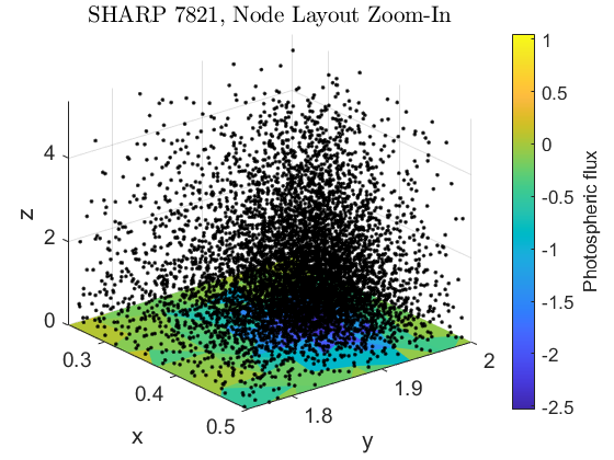
A novel methodology to scatter nodes variably in space while retaining quasiuniform clustering has been the focus of recent research, and we apply state of the art advancing-front technique per van der Sande & Fornberg (2021). A zoom-in on a portion of the domain of one simulation is given in Figure 1.
The clustering density of the method depends on an exclusion radius; the higher the function value, the sparser the node placement. We scale this quantity according to
| (1) |
where is a smoothed version of constructed via a maximal binning window and normalized to have a maximum value of , and is the ratio of the length of the longer transverse side of the domain to the shorter one (the domain is computationally normalized for the shortest side to be length ). Note that this algorithm generates nodesets with variable total numbers of nodes; is an upper bound for this quantity which is occasionally obtained, but most members of the PARSE dataset fall slightly below that threshold.
2.4 Numerical Model
The active region is extrapolated as a solution to the magnetohydrostatic equations, namely
| (2) |
We consider this a heterogeneous forced equation in terms of the conservative plasma forcing field .
The numerical model used for the extrapolations in this repository is described in detail in Mathews et al. (2022), and the curious reader is directed to that work. Here we discuss in detail only the model setup and determination of tunable parameters.
-
•
The photospheric boundary is informed by the SHARP, as described in Section 2.2. Furthermore, a radiative condition is enforced at the upper boundary, . And the side boundaries have wave-permissible bounary conditions, , the normal vector to the given boundary.
-
•
The numerical model uses a fixed hyperviscocity parameter to remediate numerical noise in the solution; a value of has been selected for this purpose.
-
•
The model resolves and computes a set of nonphysical “ghost nodes” below the solar surface. These nodes are necessary for the extrapolation technique, but their fields are not considered physical, and they have been omitted from the published data.
-
•
Finally, we find that the auxiliary equation solution included in the original method to remove any small divergence in the field converged poorly on the scattered domain, and has been omitted from calculations. This means that the domain is not necessarily totally free of magnetic divergence, but we note in Section 3 that the effect of this omission is negligible.
2.5 Plasma prescription
The numerical model allows for different selections of to be chosen and so poll the different possible topologies of the magnetic field configurations which can be extrapolated from the photospheric observations. However, the choice of plasma is not well-determined from the observations available. Indeed, determination of the correct magnetic field configuration is likely to be partially the task of the machine learning algorithm based on available auxiliary information.
Instead, we select a suite of possible plasma distributions, determined by 100 scattered volumetric collocation points. Such a determination is considered possible if it satisfies the nullspace equation
| (3) |
at the surface. This is accomplished by taking the QR factorization of the transpose of the linear system in (3) and taking a random subset of the columns of which correspond to diagonal elements of below a threshold ( was determined suitable for this purpose). This has the benefit of selecting plasmas which are orthonormal in terms of their volumetric collocation points, allowing more representative sampling of the model output space.
For purposes in which the plasma can be discounted, or the variations in magnetic topology not sufficiently interesting, a non-linear force-free extrapolation is included for each SHARP, obtained with an otherwise identical algorithm (the pressure is just set uniformly to ).
3 Dataset Analysis
We obtain strong convergence of MHS balance across all but a small subset of solutions. For most SHARPs, the solutions are topologically similar across plasma prescriptions, but with small deviations in loop height or volumetric structure. As can be observed in the three solutions in Figure 2, the forced fields are usually more complicated, pushed down closer to the photosphere, and have more transverse action, with field lines often leaving through the sides of the computational box. In some cases, such as the right panel in the same figure, the numerical hyperdiffusion was insufficient to remove all numerical artifacting, and we observe some small-scale field spirals. These are typically only in outbound open field lines, which are poorly constrained by the upper boundary conditions alone.


4 Dataset Structure and Access
Each solution is saved as a separate FITS file. The FITS file has a collection of Image Header Data Units (HDUs) which correspond to different physical parameters, described in Table 1. Each is a one-dimensional array with entries corresponding to the scattered nodes. The header data of the primary HDU contains information about the simulation or active region, and is detailed in Table 2.
| NAME | DESCRIPTION |
|---|---|
| MAIN | Primary HDU, containing no data but the header has |
| meta-information about the SHARP or simulation. | |
| BX | component of the magnetic field |
| BY | component of the magnetic field |
| BZ | component of the magnetic field |
| NODEX | coordinate at which the physical values are defined |
| NODEY | coordinate at which the physical values are defined |
| NODEZ | coordinate at which the physical values are defined |
| FX | component of the plasmatic forcing |
| FY | component of the plasmatic forcing |
| FZ | component of the plasmatic forcing |
| NAME | DESCRIPTION |
|---|---|
| SIM_N | The total number of nodes (i.e., the length of each column vector of physical parameters). |
| SIM_L2 | Residual of the magnetohydrostatic simulation, in nodecount-normalized L2 norm. |
| Provided as a proxy of simulation convergence; higher values may yield less physical solutions. | |
| Can be interpreted as a net force on the system exerted by the Lorentz and plasma forcing. | |
| The force-free field has a ‘NULL’ entry. | |
| LEN_X | Size of the dimension of the computational box, in meters |
| LEN_Y | Size of the dimension of the computational box, in meters |
| LEN_Z | Size of the dimension of the computational box, in meters (the height) |
| LEN_UNIT | Unit of LEN_X, LEN_Y and LEN_Z |
| SHARPNUM | The SHARP number for the active region |
| ARNUM | The NOAA Active Region number for the active region, if it exists in the catalogue. |
| This is a string, and sometimes is ‘MISSING’ or contains more than one NOAA Active Region number. | |
| TAI_REC | The TAI date and time the active region was imaged, in the form ‘YYYY.MM.DD_HH:MM:SS’. |
| USFLUX | Unsigned flux in the active region |
| AREA | The area of the de-projected SHARP patch in micro-hemispheres. |
| LON_MIN | Minimum longitude of the active region (Stonyhurst). |
| LAT_MIN | Minimum latitude of the active region (Stonyhurst). |
| LON_MAX | Maximum longitude of the active region (Stonyhurst). |
| LAT_MAX | Maximum latitude of the active region (Stonyhurst). |
| S_NAXIS1 | Number of pixels along axis 1 of the original SHARP image |
| S_NAXIS2 | Number of pixels along axis 2 of the original SHARP image |
| S_CRPIX1 | X coordinate of disk center with respect to lower-left corner (in pixels) of the original SHARP image |
| S_CRPIX2 | Y coordinate of disk center with respect to lower-left corner (in pixels) of the original SHARP image |
| S_CRVAL1 | X origin of the original SHARP image: (0,0) at disk center |
| S_CRVAL2 | Y origin of the original SHARP image: (0,0) at disk center |
| S_CUNIT1 | unit of S_CDELT1 |
| S_CUNIT2 | unit of S_CDELT1 |
| S_CDELT1 | scale in the x direction of the original SHARP image |
| S_CDELT2 | scale in the y direction of the original SHARP image |
| VERSION | A version number for the PARSE dataset, to allow distinguishing later updates to the simulations; |
| the set described in this paper is Version 1.0.0. |
Each SHARP is associated with a number of FITS files, indexed in the filename after the SHARP number. The index corresponds to the force-free solution, and the others after that are forced. For the 1.0.0 release, six forced solutions for each SHARP are provided.
The PARSE dataset is available open access on Zenodo (doi 10.5281/zenodo.8213061). The data generation code and example files that read the data are available on github at https://github.com/apt-get-nat/PARSE .
5 Future Work
The dataset is being continuously updated with more SHARPs. It should be possible to complete the dataset with an extrapolation of a single time frame from every extant SHARP active region by the end of 2024. We also wish to include a greater number of plasma-prescribed extrapolations for each observation to better capture the full range of possible topologies.
A future goal may also be to increase the resolution of the extrapolations. points can be considered a coarse resolution for some numerical use cases, and while it has proved sufficient for quantitative results (Mathews et al., 2020), resolutions an order of magnitude higher would doubtless yield more physical magnetic fields.
6 Acknowledgements
This work was funded by the NASA Postdoctoral Program Fellowship, which is administered by Oak Ridge Association of Universities.
This work is based heavily on the SHARP dataset, and would not have been possible without the careful collection, stewardship and processing of that data by Monica Bobra and Stanford University.
Finally, this work was greatly aided by the temporary provision of computing resources by HP and Nvidia.
References
- Bobra et al. (2014) Bobra, M. G., Sun, X., Hoeksema, J. T., et al. 2014, Solar Physics, 289, 3549
- Mathews et al. (2020) Mathews, N. H., Flyer, N., & Gibson, S. E. 2020, The Astrophysical Journal, 898, 70
- Mathews et al. (2022) —. 2022, Journal of Computational Physics, 462, 111214, doi: https://doi.org/10.1016/j.jcp.2022.111214
- van der Sande & Fornberg (2021) van der Sande, K., & Fornberg, B. 2021, SIAM Journal on Scientific Computing, 43, A242