The PFS view of TOI-677 b: A spin-orbit aligned warm Jupiter in a dynamically hot system111This paper includes data gathered with the 6.5 meter Magellan Telescopes located at Las Campanas Observatory (LCO), Chile.
Abstract
TOI-677 b is part of an emerging class of “tidally-detached” gas giants () that exhibit large orbital eccentricities and yet low stellar obliquities. Such sources pose a challenge for models of giant planet formation, which must account for the excitation of high eccentricities without large changes in the orbital inclination. In this work, we present a new Rossiter-McLaughlin (RM) measurement for the tidally-detached warm Jupiter TOI-677 b, obtained using high-precision radial velocity observations from the PFS/Magellan spectrograph. Combined with previously published observations from the ESPRESSO/VLT spectrograph, we derive one of the most precisely constrained sky-projected spin-orbit angle measurements to date for an exoplanet. The combined fit offers a refined set of self-consistent parameters, including a low sky-projected stellar obliquity of and a moderately high eccentricity of , that further constrains the puzzling architecture of this system. We examine several potential scenarios that may have produced the current TOI-677 orbital configuration, ultimately concluding that TOI-677 b most likely had its eccentricity excited through disk-planet interactions. This system adds to a growing population of aligned warm Jupiters on eccentric orbits around hot ( K) stars.
1 Introduction
In contrast to the alignment of the solar spin and the planetary orbits in our solar system (Souami & Souchay, 2012), exoplanets have been discovered on inclined, polar (e.g. Anderson et al., 2018; Addison et al., 2018; Bourrier et al., 2020; Albrecht et al., 2021; Watanabe et al., 2022) or even retrograde (e.g. Neveu-VanMalle et al., 2014; Temple et al., 2017, 2019) orbits around their host stars. The degree of the spin-orbit (mis)alignment of a planetary system is quantified by the "stellar obliquity", which is the angle between the planetary orbital angular momentum vector and the stellar spin angular momentum vector. The obliquity of a system is sculpted by both its degree of and mechanism for dynamical excitation, as well as subsequent tidal effects (see Ogilvie (2014) for a review of tidal dissipation). Obliquity excitation mechanisms fall into three categories (Albrecht et al., 2022): primordial misalignment of the proto-planetary disk (Matsakos & Königl, 2017; Takaishi et al., 2020; Romanova et al., 2021), post-formation misalignment (Anderson et al., 2016; Petrovich & Tremaine, 2016; Anderson & Lai, 2018; Teyssandier et al., 2019; Beaugé & Nesvorný, 2012), and changes in the stellar spin that are not related to planet formation (Rogers et al., 2012, 2013).
Stellar obliquities are commonly constrained using the Rossiter-McLaughlin effect (Rossiter, 1924; McLaughlin, 1924), which enables measurements of the sky-projected spin-orbit angle . A planet blocks out blue-shifted or red-shifted components of the rotating host star’s light at different phases during its transit, resulting in a deviation from the overarching Doppler reflex motion in the host star’s spectrum (Queloz et al., 2000). High-resolution spectroscopic observations across the transit can be leveraged to measure the Rossiter-McLaughlin effect.
To date, measurements of the stellar obliquity have been severely biased toward systems hosting a massive and close-orbiting () planet, which are referred to as “hot Jupiters”, due to their frequent, short, and deep transits (see Albrecht et al. (2022) for a review of existing constraints). Only a handful of wider-orbiting “warm Jupiter” systems () have precise spin-orbit constraints due to their low transit probabilities, long transit durations, and infrequent transit events. However, the orbital configurations of warm-Jupiter systems can play an important role in constraining the prevalence of competing planet formation and evolution pathways (Winn & Fabrycky, 2015; Dawson & Johnson, 2018).
A comparison between the orbital configurations of close-orbiting hot Jupiters and wide-orbiting warm Jupiters (such as the orbital eccentricity distribution, the companion rate, and so on) can shed light on the prevalence of different formation mechanisms for these two types of planets. The possible formation channels for hot and warm Jupiters are directly comparable: each class of planets could potentially arise through in situ formation, disk migration, or high-eccentricity migration. Previous work has shown that high-eccentricity tidal migration triggered by planet-planet or planet-star Kozai-Lidov cycles (KL; von Zeipel, 1910; Lidov, 1962; Kozai, 1962; Wu & Murray, 2003; Naoz et al., 2011, 2012; Naoz, 2016) is a promising channel to account for the observed properties of hot Jupiters on a population level (Winn & Fabrycky, 2015; Dawson & Johnson, 2018; Rice et al., 2022).
However, it is not yet clear how warm Jupiters fit into this emerging picture. Warm Jupiters, by contrast to hot Jupiters, show a high occurrence rate of nearby planetary companions (Huang et al., 2016; Wu et al., 2023). Furthermore, previous work has proposed that the warm Jupiter eccentricity distribution contains both a low-eccentricity component and a roughly uniform component (Dawson & Johnson, 2018; Petrovich & Tremaine, 2016). In situ formation or disk migration could account for the low-eccentricity component of this distribution, producing warm Jupiters that cannot be excited by subsequent scattering (Petrovich et al., 2014). A separate mechanism is needed to reproduce the uniform eccentricity distribution component, which is also difficult to reproduce in the high-eccentricity migration framework as warm Jupiters are tidally detached from their host stars.
A comparison of the stellar obliquity distributions of hot and warm Jupiters, particularly around hot stars, can help to distinguish the prevalence of each mechanism by disentangling the stage at which misalignments arise (Triaud, A. H. M. J. et al., 2010; Hamer & Schlaufman, 2022; Attia et al., 2023). Hot Jupiters on tight orbits are strongly affected by tidal interactions with their host stars, such that the outer layer of the star may realign over time (Winn et al., 2010; Albrecht et al., 2012). Previous studies of hot Jupiter stellar obliquities exhibit evidence suggestive of tidal realignment (Albrecht et al., 2012): hot stars hosting hot Jupiters span a wider range of obliquities than their cool star counterparts (Schlaufman, 2010; Winn et al., 2010). The transition occurs at the Kraft break ( K), the dividing point for whether the stellar envelope is convection-dominated or radiation-dominated (Kraft, 1967).
By contrast, warm Jupiters are expected to be “tidally detached” – that is, they are relatively unaffected by tidal dissipation within the age of the system, such that they offer valuable insights into the primordial obliquity distribution at the time of planet formation (Zhou et al., 2020; Rice et al., 2021). Rice et al. (2022a) suggests that small spin–orbit angles observed for warm Jupiters around single stars may indicate that protoplanetary disks tend to be aligned at the time of gas dispersal, while hot Jupiters are misaligned through dynamical interactions after the disk has dispersed. A larger sample of warm Jupiters with precisely measured spin-orbit orientations – particularly those around hot stars, which have relatively few such measurements to date – will enable us to examine the robustness of this preliminary statistical result and to further inform the key hot vs. warm Jupiter obliquity excitation mechanism(s).
The precise characterization of individual warm Jupiter orbital configurations is critical to inform competing models for the formation of warm Jupiters more generally. TOI-677 (TIC 280206394) was first identified as a planet-hosting candidate by the TESS mission (Ricker et al., 2015) and was then characterized by Jordán et al. (2020) as a bright (), hot ( K) late-F star hosting a wide-orbiting eccentric () gas giant TOI-677 b. Recently, Sedaghati et al. (2023) reported a sky-projected obliquity measurement () for this target over a single transit with the ESPRESSO (Echelle Spectrograph for Rocky Exoplanets and Stable Spectroscopic Observations; Pepe et al., 2021) spectrograph.
We present a new, independent Rossiter–McLaughlin measurement across one transit of TOI-677 b with the Carnegie Planet Finder Spectrograph (PFS; Crane et al., 2006, 2008, 2010) on the 6.5m Magellan Clay telescope. This observation was obtained as part of the Stellar Obliquities in Long-period Exoplanet Systems (SOLES) survey (Rice et al., 2021; Wang et al., 2022; Rice et al., 2022b, 2023a; Hixenbaugh et al., 2023; Dong et al., 2023; Wright et al., 2023; Rice et al., 2023b; Lubin et al., 2023), and it represents the tenth published result from this program.
We examine our new measurement, together with archival observations and data from Jordán et al. (2020) and Sedaghati et al. (2023), to refine the orbital parameters and the stellar obliquity of the TOI-677 system. By combining two independent RM datasets, each from high-precision spectrographs on 6-8m class telescopes, we derive one of the most precisely constrained sky-projected spin-orbit measurements to date: an important advance toward inferring precise orbital geometries and understanding the true dispersion of exoplanet orbital distributions. We find that TOI-677 b is well aligned with its host star, with .
2 Observations
2.1 PFS Observations
We observed the Rossiter-McLaughlin effect across one full transit of TOI-677 b from UT 2:19-9:24 on February 10th, 2023 using the Carnegie Planet Finder Spectrograph (PFS; Crane et al., 2006, 2008, 2010) on the 6.5m Magellan Clay telescope. In addition to the transit itself, our observation included 2.5 hours of pre-transit and 2 hours of post-transit baseline observations. Seeing was highly variable across the observing sequence, ranging from . The target was high in the sky, at airmass during the start of the observing sequence and reaching at the end. The moon was separated from the target by throughout the night.
The spectral data reduction and RV extraction were performed using a customized pipeline (Butler et al., 1996). The PFS radial velocity values and uncertainties used in this work are listed in Table 1.
| BJD (-2,450,000) | RV (m/s) | (m/s) |
|---|---|---|
| 9985.604119 | 89.06 | 3.89 |
| 9985.613910 | 90.47 | 3.48 |
| 9985.623650 | 79.87 | 3.56 |
| 9985.633890 | 65.70 | 3.29 |
| 9985.643931 | 69.94 | 2.97 |
| 9985.653941 | 63.16 | 2.82 |
| 9985.664041 | 48.56 | 2.70 |
| 9985.673402 | 46.57 | 2.90 |
| 9985.683612 | 38.34 | 2.79 |
| 9985.693662 | 30.57 | 2.51 |
| 9985.703572 | 27.52 | 2.58 |
| 9985.713363 | 23.82 | 2.36 |
| 9985.723783 | 26.02 | 2.73 |
| 9985.733683 | 16.15 | 2.66 |
| 9985.743514 | 0.00 | 2.70 |
| 9985.753874 | -9.34 | 2.52 |
| 9985.763624 | -28.07 | 2.62 |
| 9985.773135 | -46.97 | 3.17 |
| 9985.783905 | -65.26 | 3.13 |
| 9985.793885 | -75.57 | 3.31 |
| 9985.803656 | -59.33 | 3.37 |
| 9985.813456 | -66.81 | 3.46 |
| 9985.823726 | -68.57 | 3.60 |
| 9985.833226 | -66.60 | 3.91 |
| 9985.843987 | -78.43 | 3.91 |
| 9985.854247 | -92.25 | 3.36 |
| 9985.863747 | -91.11 | 3.52 |
| 9985.873578 | -99.67 | 3.49 |
| 9985.883508 | -101.34 | 3.72 |
Note. — This table is available in machine-readable form in the online manuscript.
2.2 TESS Photometry
TOI-677 (TIC 20182165) was observed at a two-minute cadence in TESS Sectors 9, 10, 35, 36, 62, and 63, including 12 transits in total. We downloaded the two-minute cadence SPOC TESS data from the Mikulski Archive for Space Telescopes (MAST) Portal 222https://mast.stsci.edu/portal/Mashup/Clients/Mast/Portal.html. We then detrended the TESS light curves to remove systematic trends by fitting a Gaussian Process (GP) model to the out-of-transit light curves using the juliet Python package (Espinoza et al., 2019), which implements the Python package celerite (Foreman-Mackey et al., 2017) to build the GP model. The detrended TESS data used for the analysis is presented in Table 2. The phase-folded TESS light curve, along with the best-fit model from the combined fit in Table 4, is shown in the leftmost panel of Figure 1.
| BJD (-2,450,000) | Flux (ppt) | (ppt) |
|---|---|---|
| 8543.885982 | -0.938 | 0.819 |
| 8543.887371 | -0.235 | 0.819 |
| 8543.888760 | -2.335 | 0.818 |
| 8543.890148 | -1.285 | 0.818 |
| 8543.891537 | -1.345 | 0.818 |
| 8543.892926 | -1.256 | 0.818 |
| 8543.894315 | -1.257 | 0.818 |
| 8543.895704 | -0.869 | 0.817 |
| 8543.897093 | -1.712 | 0.817 |
| 8543.898482 | -0.338 | 0.817 |
| 8543.899871 | 0.401 | 0.817 |
| 8543.901260 | -0.503 | 0.817 |
| 8543.902649 | -1.412 | 0.816 |
| 8543.904038 | -0.585 | 0.816 |
| 8543.905426 | 0.500 | 0.816 |
| … | … | … |
Note. — This table is available in machine-readable form in the online manuscript.
2.3 LCO Ground-based Photometry
We obtained photometry of TOI-677 that was simultaneous with the RM observation using two 1m and two 0.4m telescopes within the Las Cumbres Observatory Global Telescope (LCOGT; Brown et al., 2013) network on UT February 10th, 2023. All LCOGT observations were obtained with the Pan-STARRS filter.333https://lco.global/observatory/instruments/filters/PanSTARRS-zs/ One of the 1m telescopes did not successfully defocus and nearly saturated the target star; however, a reasonable lightcurve could still be extracted. The second 1m telescope, as well as the two 0.4m telescopes, successfully defocused with no problems. The images were calibrated by the standard LCOGT BANZAI pipeline (McCully et al., 2018) and differential photometric data were extracted using AstroImageJ (Collins et al., 2017). The detrended LCO data used for the analysis are presented in Table 3. We combined photometry from telescopes of the same diameter into one dataset (labeled as “LCO 1m” and “LCO 0.4m”) in our analysis. The phase-folded LCO light curves from the 1m and 0.4m telescopes, along with the best-fitting model from the combined fit (see Table 4), are shown in the third and fourth panels in Figure 1.
| BJD (-2,450,000) | Flux (ppt) | (ppt) | Telescope |
|---|---|---|---|
| 9985.664765 | 1.544 | 3.481 | LCO 0.4m (1) |
| 9985.665403 | 1.483 | 3.483 | LCO 0.4m (1) |
| 9985.666047 | 8.032 | 3.488 | LCO 0.4m (1) |
| 9985.666682 | -0.989 | 3.453 | LCO 0.4m (1) |
| 9985.667324 | 6.566 | 3.482 | LCO 0.4m (1) |
| … | … | … | … |
| 9985.664785 | -3.179 | 3.383 | LCO 0.4m (2) |
| 9985.665528 | 10.224 | 3.378 | LCO 0.4m (2) |
| 9985.666258 | 6.324 | 3.392 | LCO 0.4m (2) |
| 9985.666981 | 5.986 | 3.390 | LCO 0.4m (2) |
| 9985.667688 | 4.987 | 3.378 | LCO 0.4m (2) |
| … | … | … | … |
| 9985.664984 | 0.617 | 0.713 | LCO 1m (1) |
| 9985.665619 | 1.120 | 0.711 | LCO 1m (1) |
| 9985.666269 | 0.606 | 0.710 | LCO 1m (1) |
| 9985.666856 | 0.221 | 0.710 | LCO 1m (1) |
| 9985.667443 | 0.213 | 0.711 | LCO 1m (1) |
| … | … | … | … |
| 9985.664894 | -1.433 | 0.698 | LCO 1m (2) |
| 9985.665489 | -1.568 | 0.698 | LCO 1m (2) |
| 9985.666078 | -1.877 | 0.698 | LCO 1m (2) |
| 9985.666671 | -1.811 | 0.698 | LCO 1m (2) |
| 9985.667260 | -1.793 | 0.699 | LCO 1m (2) |
Note. — The table is in machine-readable form in the online manuscript.

3 Analysis and Results
| Parameter | Priors | PFS | ESPRESSO | Combined Fit |
|---|---|---|---|---|
| Fitted Parameters: | ||||
| (BJD-2458500) | ||||
| (day) | ||||
| (m/s) | ||||
| (km/s) | ||||
| … | ||||
| … | ||||
| … | ||||
| … | ||||
| Stellar Parameter Priors: | ||||
| … | … | … | ||
| … | … | … | ||
| Derived Parameters: | ||||
| … | ||||
| … | ||||
| … | ||||
| … | ||||
| (hours) | … | |||
| … | ||||
| … | ||||
| … | ||||
| (au) | … | |||
| … | ||||
| … | ||||
| … | ||||
| … | ||||
| … | ||||
| … | ||||
| … | ||||
| … | ||||
| … | … | |||
| … | … | |||
| … | … | |||
| … | … |

We carried out three independent joint fits using in-transit RV data only from PFS, only from ESPRESSO, and from both telescopes together. Each of these fits included photometric data from TESS and LCO (see Section 2), as well as archival photometric data from SSMKO (see the second panel in Figure 1) and archival RV data from the FEROS, Coralie, CHIRON, NRES, and Minerva-Australis spectrographs. The in-transit PFS RV data are provided in Table 1, and the in-transit ESPRESSO RV data are adopted from Table 4 in Sedaghati et al. (2023). The SSMKO photometry data and all other archival RV data are drawn from Tables 2 and 4 in Jordán et al. (2020).
Our fits each used allesfitter (Günther & Daylan, 2021), which is a powerful tool for jointly modeling photometric and RV data. Allesfitter constructs a Bayesian inference framework that unites the ellc (light curve and RV models; Maxted (2016)) and emcee (Markov Chain Monte Carlo (MCMC) sampling; Foreman-Mackey et al. (2013a)) Python packages, building a joint model of photometry and radial velocities to fit the Rossiter-McLaughlin effect.
All fitted parameters listed in Table 4 were allowed to vary and were initialized with uniform priors , with a lower bound and an upper bound . is the planet-to-star radius ratio; is the sum of radii divided by orbital semimajor axis; is the cosine of the orbital inclination; is the mid-transit epoch; is the orbital period; is the RV semi-amplitude; and are the eccentricity parameters; is the stellar rotation velocity projected on the line of sight; is the sky-projected stellar obliquity; and are the quadratic limb darkening coefficients (Kipping, 2013) treated separately for all instruments that captured transit signals (TESS, SSMKO, LCO 1m, LCO 0.4m, PFS, and ESPRESSO). The initial values for , , , , , , , and were adopted from Jordán et al. (2020).
The sky-projected spin-orbit angle was initialized as and was allowed to vary between and . The two limb-darkening coefficients and were initialized with values of 0.5 and were only allowed to vary between 0 and 1. Jitter terms were modeled separately for each instrument and were added in quadrature to the formal uncertainties. The baseline model was evaluated separately for photometric and radial velocity data. We allowed for a constant offset with priors bounded between -0.1 and 0.1 in relative flux units for photometric data. For RV data, we adopted a linear baseline model, as previous work has identified a significant long-term trend in the radial velocities which could be caused by an outer companion (Jordán et al., 2020). We assigned a general linear slope for the archival radial velocities and different linear slopes for the PFS and ESPRESSO datasets. The constant RV offsets were different for individual spectrographs and were allowed to vary between -1 km/s and 1 km/s.
Stellar parameter priors are needed for the derived parameters, both listed in Table 4. We adopted Gaussian priors for the host star’s mass and radius drawn from Jordán et al. (2020), where they were derived from a combination of spectroscopy, spectral energy distribution (SED), and isochrone fits. The derived parameters are the planetary radius (), planetary mass (), planetary semi-major axis over host star radius (), impact parameter (), total transit duration (), inclination of the planetary orbit (), eccentricity (), argument of periastron (), semi-major axis (), and the re-parameterized quadratic limb darkening coefficients and for TESS, SSMKO, LCO 1m, LCO 0.4m, PFS, and ESPRESSO.
We ran an affine-invariant MCMC analysis for each of our three joint fits, with 150 walkers to sample the posterior distributions of all model parameters. We ensured that each chain was fully converged by running all Markov chains to over 30 times their autocorrelation length, which corresponded to a minimum of 250,000 accepted steps per walker.
The values and 1- uncertainties of fitted parameters are listed in Table 4. The best-fit joint models are shown in Figure 2, together with the values and uncertainties for each measurement. The jitter term for each instrument has been incorporated into the error bar of the plotted data points.
The sky-projected spin-orbit angles derived from PFS, ESPRESSO, and the combined fit are , , and respectively. These values are consistent with each other within 2-, and our final, combined fit measurement is also consistent with the result from Sedaghati et al. (2023) within 2-. TESS out-of-transit light curves of TOI-677 are nearly flat and bear no significant periodicities that could be attributed to the stellar spin, preventing a further derivation of the true 3D spin-orbit angle .
While the PFS measurement alone is suggestive of a solar-system-like stellar obliquity ( away from alignment; Souami & Souchay (2012)), the ESPRESSO measurement alone is more indicative of exact alignment. Our final result, which combines the two, lies at an intermediate value between these two possibilities. The 2- discrepancy between values from the PFS and ESPRESSO measurements is discussed in detail in Section 4.3.
4 Discussion
4.1 Potential formation channels
TOI-677 b displays a surprising orbital geometry: while it is a warm Jupiter on a substantially eccentric orbit () around a hot star ( K; Jordán et al., 2020), suggesting potential dynamical upheaval, the planet’s orbit is precisely aligned with the host star’s spin in its sky-plane projection (). One possibility is that TOI-677 b may have had its orbital eccentricity excited through planet-disk interactions. Alternatively, the long-term linear RV trend followed by TOI-677 indicates the likely presence of an unconfirmed outer brown dwarf companion in the system (see Table 3 in Sedaghati et al. (2023)), which may have played a role in exciting TOI-677 b’s eccentricity. The Coplanar High-Eccentricity Migration (CHEM, Petrovich, 2015) mechanism or Kozai-Lidov (KL) oscillations (Fabrycky & Tremaine, 2007; Naoz et al., 2011, 2012) may each potentially account for the formation of aligned (), moderately eccentric () warm Jupiters with an outer companion.
In the following subsections, we discuss each of these possible formation channels and the conditions under which they are effective. Ultimately, we find that the CHEM and KL mechanisms are unlikely to produce the observed system configuration, leaving planet-disk interactions as the leading hypothesis. The properties of the companion brown dwarf may offer further evidence to distinguish between potential formation channels for TOI-677 b.
4.1.1 Coplanar High-Eccentricity Migration
Coplanar high-eccentricity migration, or CHEM (Petrovich, 2015; Zink & Howard, 2023), offers one avenue to produce highly eccentric warm Jupiters within the plane of the natal protoplanetary disk. In the CHEM framework, a moderately or highly eccentric outer companion can excite the inner planet’s eccentricity in-situ when the mutual inclination between the planet’s orbit and the companion’s orbit is small ().
Following the arguments of Sedaghati et al. (2023), the measured eccentricity of the companion fails to excite the eccentricity of the inner planet to the new value from our combined fit. Therefore, the CHEM mechanism would struggle to account for TOI-677 b’s configuration unless the companion’s eccentricity is found to be substantially higher than this previous estimate.
4.1.2 Formation through the KL mechanism followed by tidal dissipation
The Kozai-Lidov (KL) mechanism followed by tidal dissipation offers another potential avenue to produce aligned and substantially eccentric warm Jupiters. Hierarchical three-body systems, where the ratio of inner and outer orbital semimajor axes is much smaller than unity, may undergo KL oscillations over secular timescales. During these oscillations, the mutual inclination between the inner and outer orbits is traded back and forth with the inner orbit’s eccentricity such that the component of the inner planet’s orbital angular momentum parallel to that of the perturber () is conserved as (e.g. Tremaine, 2023)
| (1) | ||||
where is the mass of the host star, is the semimajor axis of the planet (which remains unchanged due to energy conservation), is the eccentricity of the planet, and is the mutual inclination between the planet’s and the perturber’s orbital planes.
From Equation 1, we can see that the KL mechanism offers a pathway to produce a considerable increase in the inner planet’s eccentricity in exchange for a small change in the system’s mutual inclination . Under the assumption that planets generally form in protoplanetary disks well aligned with their host stars, small changes in the mutual inclination are equivalent to small stellar obliquities . If the initial mutual inclination is larger, a smaller change in the mutual inclination is needed to excite the eccentricity from 0 to a set value through the KL mechanism.
| Description | Parameter | Value |
|---|---|---|
| The inner planet | ||
| Eccentricity | 0.460 | |
| Orbital period | (day) | 11.2365985 |
| Semi-major axis | (au) | 0.1041 |
| Argument of periapsis | 72.9 | |
| Mass | 1.234 | |
| Radius | 1.170 | |
| The outer companion | ||
| Eccentricity | 0.436 | |
| Orbital period | (day) | 4901.13876 |
| Semi-major axis | (au) | 5.9872 |
| Argument of periapsis | -123.68 | |
| Mass | 49.99 | |
| The host star | ||
| Mass | 1.158 | |
| Radius | 1.281 |
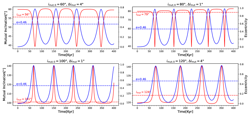
We conducted numerical integrations for the inner planet’s orbit using Kozaipy444https://github.com/djmunoz/kozaipy to confirm our argument. The starting orbital configurations for the simulations, except that the eccentricity of the inner planet is set to nearly zero (), are the same as the current observed orbital configurations listed in Table 5 . We ran the simulation for four different initial mutual inclinations , and . Our results are shown in Figure 3, with the eccentricity oscillation shown in blue and the mutual inclination oscillation shown in red. The blue dashed line marks the current, observed eccentricity (0.46) of the inner planet, while the red dashed line marks the mutual inclinations when the eccentricity reaches the observed value in the KL cycles. For initial values , and , the mutual inclinations only change by , and , respectively, for the eccentricity to reach the currently observed value. All of these values are consistent with the near-aligned stellar obliquity suggested by our combined fit measurement .
One caveat in invoking the KL mechanism is that the torque exerted on the planet from the perturber in the KL mechanism is dependent on the pericenter argument of the planet (). On close-in orbits, precessions of the pericenter argument caused by other forces including general relativistic effects (), rotational bulges (), and tidal deformations () are strong and may suppress the KL oscillations. Wu & Murray (2003) summarizes the relative precession rates for general relativistic effects, rotational bulges, and tidal deformations as
| (2) | ||||
where notations are the same as in Table 5. If any of these ratios exceeds unity, the KL oscillation is destroyed.
For the current orbit of TOI-677 b as listed in Table 5, the relative precession rates of the rotational bulges and tidal deformations both exceed unity, such that the planet’s eccentricity cannot have been excited through the KL mechanism at its current location. However, it is possible that TOI-677 b’s eccentricity was excited through the KL mechanism from an initial orbit further out in the system, and that the planet then migrated to its current position through tidal dissipation. During this migration process, the KL oscillation would be gradually quenched by higher-frequency precessions associated with general relativistic effects, rotational bulges, and tidal deformations. This is the same scenario as the high-eccentricity migration mechanism for hot Jupiters, except that the starting position is closer and the maximum eccentricity needed is lower (e.g. Wu et al., 2023). During tidal dissipation, the orbital angular momentum is conserved as (Dawson & Johnson, 2018)
| (3) |
For different starting positions, we use Equation 3 to estimate the maximum KL-excited eccentricity that must be reached to attain TOI-677 b’s current observed orbital configuration. From this, we estimate the minimum initial mutual inclination required to excite the eccentricity from 0 to through the KL mechanism if the change in the mutual inclination is within 3- of the measured value (). We also inspect whether the eccentricity evolution timescale , during which the eccentricity changes from to the current observed value , is shorter than the age of the system (about 3 Gyr from Sedaghati et al. (2023)). We calculated the eccentricity evolution timescale using Equation (6) to (13) in Rice et al. (2022), adopting an effective tidal dissipation parameter and Love number for TOI-677 b. Our calculated values for four sample initial orbital separations are listed in Table 6.
| Parameter | Values | |||
|---|---|---|---|---|
| (au) | 0.2 | 0.3 | 0.4 | 0.5 |
| 0.0386 | 0.0076 | 0.0024 | 0.0010 | |
| 0.3283 | 0.0128 | 0.0013 | 0.0002 | |
| 0.1182 | 0.0046 | 0.0005 | 0.0001 | |
| 0.76 | 0.85 | 0.89 | 0.91 | |
| 7.79 | 7.43 | 7.28 | 7.19 | |
| 76.3 | 81.4 | 83.5 | 84.6 | |
| 34.4 | 15.5 | 9.2 | 6.2 | |
If TOI-677 b had its eccentricity excited through the KL mechanism and then migrated to its current orbit through tidal dissipation, the angle between the planet’s and companion’s orbital planes () should fall within the range .
An important complication in this scenario is that, after the KL oscillation is quenched, the highly-inclined outer companion will cause the inner planet’s orbit to undergo nodal precession, altering the inner planet’s spin-orbit orientation and changing the true stellar obliquity (e.g. Yee et al., 2018; Bailey & Fabrycky, 2020). The precession rate of the longitude of the ascending node of the inner planet () can be calculated as (see Equation 3 in Yee et al., 2018)
| (4) |
where is the mean motion of the inner planet, and the meaning of other symbols is the same as above. The nodal precession period of the current orbital configuration is approximately 0.14 Myr – significantly shorter than the age of the system – assuming a mutual inclination . As a result, retaining a configuration with a low would imply that the KL oscillation was quenched recently such that nodal precession has not yet changed the inner planet’s orbital direction, or that the system is being observed at a low-stellar-obliquity trough in the precession cycle. While not impossible, this need for a chance timing alignment casts doubt on the KL scenario for TOI-677 b.
4.1.3 Eccentricity excitation through disk-planet interactions
A third possible explanation for TOI-677 b’s highly eccentric and aligned configuration is that the planet’s eccentricity may have been excited through disk-planet interactions within an aligned, natal protoplanetary disk. However, most previous models of disk-planet interactions have struggled to excite planetary eccentricities at the level of (e.g. Kley & Dirksen, 2006; Bitsch & Kley, 2010; Duffell & Chiang, 2015).
Recently, several works proposed that the outer disk can excite the eccentricity of a planet in an inner cavity to higher values than previously attained. Romanova et al. (2023) demonstrated that, in the presence of Lindblad resonances between an outer disk and the planet in the inner cavity, the maximum possible eccentricity is pushed up to . A caveat of this work is that the disk material cannot penetrate into the cavity, which excludes the local corotation torque that damps the planet’s eccentricity.
Li & Lai (2023) proposed that a planet within the inner cavity could, alternatively, attain a high eccentricity (between 0.1 and 0.6) through resonant interactions with a dispersing, low-eccentricity () protoplanetary disk. Although specific disk conditions, including the initial disk mass, gas temperature viscosity, and mass-loss rate, are needed for the disk to gain eccentricity through rapid cooling, this mechanism may operate in at least some regimes.
Furthermore, Murray et al. (2022) demonstrated that if a resonant planet pair migrates into the cavity, the eccentricity of the inner planet can be excited to high values () through disk-driven differential precession between the pair. In this scenario, the disk must be heavy enough to produce a high differential precession rate between the two planets in resonance, and the disk dispersal must proceed slowly enough to avoid destabilizing the resonant planet pair. The outer companion’s mass must be comparable to that of the inner planet for it to perturb the inner planet onto a high-eccentricity orbit, such that, if the resonant planet pair survived the disk dispersal, the companion’s presence should have been inferred through either direct RV signatures or transit timing variations of TOI-677 b.
While eccentricity excitation through disk-planet interactions may be promising to produce eccentric and aligned warm-Jupiter systems, further work is needed to more clearly demonstrate whether the necessary initial conditions are typically met. For an individual planet TOI-677 b, it is difficult to definitively validate that its eccentricity is excited through disk-planet interactions. Nevertheless, this scenario would be strengthened if the outer brown dwarf companion is found to be coplanar, since a mutually inclined companion would be more indicative of dynamical evolution out of the disk plane.
4.1.4 Implications for future observations
The properties of TOI-677 b’s outer companion offer important clues into potential formation scenarios for the system. The companion would most likely reside in a coplanar configuration if the eccentricity of TOI-677 b was excited through either disk-planet interactions or CHEM. Alternatively, the companion should have a substantial mutual orbital inclination with respect to the planet if TOI-677 b’s high eccentricity was excited through the KL mechanism. Through further characterization of TOI-677 c – from long-term RV observations and/or accurate astrometric characterization – it may be possible to distinguish between the system’s prospective formation channels and further clarify the origins of this enigmatic system.
We anticipate that the ongoing Gaia mission (Gaia Collaboration et al., 2016) may provide useful constraints for TOI-677 c. The astrometric signature of TOI-677 c is , about fifty times greater than the along-scan accuracy per field of view passage for its host star. Therefore, according to the rough Gaia detectability criterion in Perryman et al. (2014), at least part of the orbital motion of TOI-677 c ( yr, Sedaghati et al. (2023)) should be detectable within the Gaia mission baseline ().
4.2 The alignment of warm Jupiters in single-star systems
Rice et al. (2022b) examined the sky-projected stellar obliquity distribution in relatively isolated, single-star systems and found that, in these systems, tidally detached Jovian planets are preferentially more aligned than their closer-orbiting counterparts. Over the 20 months since that sample was developed, several more stellar obliquity measurements of tidally-detached warm Jupiter systems have been accumulated. Here, we revisit the sky-projected stellar obliquity distribution555While the sky-projected spin-orbit angle is not equivalent to the true spin-orbit angle , the 3-D stellar obliquity is related to and always closer to than the 2-D stellar obliquity (Fabrycky & Winn, 2009). Dong & Foreman-Mackey (2023) also demonstrated that, at the population level, the distribution of is roughly equivalent to the underlying distribution. Therefore, we can use the sky-projected spin-orbit angle to study the statistical properties of the stellar obliquity in close-in gas giant systems. of hot and warm Jupiters in single-star systems with these newer measurements incorporated.
Our sample consists of systems included in both the NASA Exoplanet Archive (2023) “Planetary Systems” list and the TEPCat catalog666https://www.astro.keele.ac.uk/jkt/tepcat/ (Southworth, 2011), which compiles published stellar obliquity measurements into a single database. Both datasets were downloaded on 2023 October 20. We drew and from the TEPCat catalog, and all other system parameters were drawn from the default parameter set of the NASA Exoplanet Archive. We used the most recently obtained stellar obliquity measurement for most stars, with the exception of systems in which previous measurements were much more precise. Exoplanets with no eccentricity measurements in the NASA Exoplanet Archive were excluded from the sample.
From this combined dataset, we selected gas giants in single-star systems for our analysis. Following Rice et al. (2022b), we used as the cut-off for Jovian planets, as the dividing line between close-orbiting hot Jupiters and tidally-detached warm Jupiters, and K (the Kraft break) as the boundary between hot and cool stars. Single-star systems were selected by removing any systems with sy_snum > 1 in the NASA Exoplanet Archive, as well as any systems identified with comoving companions from the Gaia DR3 catalogue (Gaia Collaboration et al., 2023) following the methods of El-Badry et al. (2021) and Rice et al. (2022b). We note that this selection explicitly removes “Saturns” () – the lowest-mass Jovian planets that previous samples have shown are more often misaligned than higher-mass Jovians, and that do not appear to follow the same trends (Rice et al., 2022b; Morgan et al., 2023).
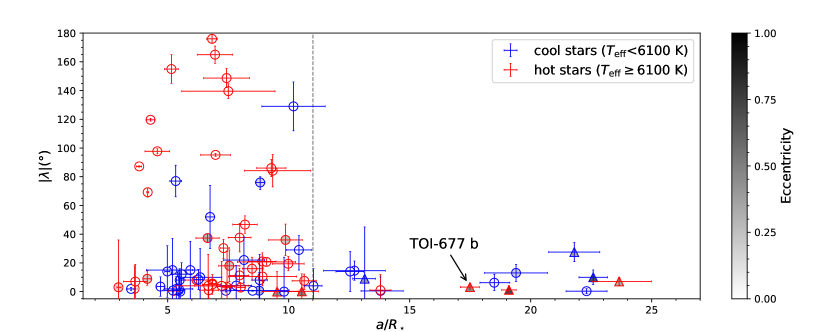
Figure 4 places TOI-677 b into context as one of the widest-separation tidally detached exoplanets with a measured value. All of the warm Jupiters in single-star systems are, so far, consistent with alignment () within 1- (Harre et al., 2023; Espinoza-Retamal et al., 2023). Despite their small spin-orbit angles, the eccentricity distribution of warm Jupiters spans a wide range of values, with an even broader dispersion than that of their close-orbiting counterparts (Yu et al., 2018).
Moreover, TOI-677 b supports the previously suggested, tentative trend that wide-orbiting Jupiters around hot stars may be preferentially more aligned than those around cool stars (Rice et al., 2021). If this trend continues to gain significance, it may be indicative of an obliquity excitation mechanism restricted to cool stars. For example, Anderson & Lai (2018) proposed that, in the presence of an external, inclined Jovian-mass companion, spin–orbit misalignments can be excited preferentially in cool-star systems due to a secular resonance between the host star’s spin axis precession frequency and nodal precession induced by interactions with the companion. Further monitoring to constrain the companion rate of misaligned warm Jupiters around cool stars would be necessary to confirm this hypothesis.
4.3 Toward an era of extreme-precision spin-orbit characterization
Existing Rossiter-McLaughlin measurements of wide-orbiting giant planets have shown that warm Jupiter exoplanets may follow an intrinsically different spin-orbit angle distribution from that of their close-orbiting counterparts (Rice et al., 2021, 2022b). However, the true distribution of spin-orbit angles for each population remains elusive due to a combination of small-number statistics and often-large uncertainties for individual measurements. Even those systems that are thought to form quiescently and would generally be classified as “aligned” demonstrate some spread in their measured spin-orbit angles (Rice et al., 2023b).
Figure 2 demonstrates that the main factor driving differences between the PFS model and the ESPRESSO model for TOI-677 b is the highest peak of the ESPRESSO dataset, where two points deviate from the rest of the trend and consequently push toward smaller values. These outliers may have originated from stellar-activity-induced jitter, demonstrating the benefit of repeat measurements when deriving fundamental parameters at high precision. In particular, our work demonstrates the importance of repeat measurements when constraining the degree of alignment of a given planetary system.
One potential alternative is that the stellar obliquity of the system may vary slightly as a function of time. This possibility has been examined in the past for the XO-3 system, where multiple measurements were discrepant by tens of degrees ( in Hébrard et al. (2008); in Winn et al. (2009); in Hirano et al. (2011)); however, Worku et al. (2022) found that there was no strong evidence for a change over time in the spin-orbit angle of XO-3 b. If present, temporal changes in the spin-orbit orientation may be caused by angular momentum transport from internal gravity waves within the host star (Rogers et al., 2012).
The origins of true low-level misalignments – which, as demonstrated by this work, must be disentangled from signatures of stellar activity – may offer insights into our own solar system’s stellar obliquity (Souami & Souchay, 2012), which lies near, but is decidedly not in exact, alignment. Analyses such as the one presented here, with more than one in-transit dataset incorporated, help to push beyond the broad population-wide regimes of “aligned” versus “misaligned” exoplanets and toward extreme-precision constraints that may demonstrate the typical degree of spin-orbit alignment across different types of planetary systems (Albrecht et al., 2022).
5 Conclusions
We have presented a new Rossiter-McLaughlin measurement of the tidally-detached warm Jupiter TOI-677 b from PFS/Magellan. We combined this new measurement with archival data, including a recently published Rossiter-McLaughlin measurement from the ESPRESSO spectrograph (Sedaghati et al., 2023), to derive a self-consistent set of updated physical parameters for TOI-677 b. Our independent observation corroborates previous findings from Sedaghati et al. (2023) that TOI-677 b exhibits a high eccentricity and yet a surprisingly low sky-projected spin-orbit angle, with values and from our combined fit.
Several formation pathways for TOI-677 b were examined through this work, each aiming to preserve the planet’s low observed sky-projected stellar obliquity while reproducing its high eccentricity. Ultimately, we find that CHEM is disfavored by the measured properties of the outer brown dwarf companion, and KL oscillations followed by tidal dissipation, while feasible, would require a low-likelihood chance alignment due to nodal precession from the outer companion. As a result, we conclude hat TOI-677 b most likely had its eccentricity excited through disk-planet interactions. Further monitoring of the outer companion – in particular, improved constraints on its mass and mutual inclination relative to TOI-677 b – would help to confirm this conjecture.
Our results expand upon previous findings from Rice et al. (2022b), showing that warm Jupiters in single-star systems continue to exhibit minimal deviation from spin-orbit alignment despite an emerging dispersion in orbital eccentricity and host star type. Ultimately, a larger population of warm Jupiters with precise spin-orbit measurements, spanning a wider range of orbital eccentricities and host star types, will be necessary to more fully demonstrate the range of orbital configurations spanned by warm Jupiters and the corresponding implications for their formation.
6 Acknowledgments
Q.H. is very grateful to Zhang Yisong at the Physics Department of Tsinghua University for his support in the discussion concerning the Kozai-Lidov oscillations. Q.H. thanks Prof. Zhu Wei from the Astronomy Department of Tsinghua University for his advice on the discussion sections. M.R. acknowledges support from Heising-Simons Foundation Grants #2023-4478 and #2023-4655, NASA grant GR122985/AWD0011072, and Oracle for Research grant No. CPQ-3033929. S.W. acknowledges support from Heising-Simons Foundation Grant #2023-4050.
This work has benefited from the use of the Grace computing cluster at the Yale Center for Research Computing (YCRC). This work makes use of observations from the Las Cumbres Observatory global telescope (LCOGT) network. Part of the LCOGT telescope time was granted by NOIRLab through the Mid-Scale Innovations Program (MSIP). MSIP is funded by NSF. This paper is based on observations made with the Las Cumbres Observatory’s education network telescopes that were upgraded through generous support from the Gordon and Betty Moore Foundation. This research has made use of the Exoplanet Follow-up Observation Program (ExoFOP; DOI: http://dx.doi.org/10.26134/ExoFOP5 (catalog 10.26134/ExoFOP5)) website, which is operated by the California Institute of Technology, under contract with the National Aeronautics and Space Administration under the Exoplanet Exploration Program. This research has made use of the NASA Exoplanet Archive (2023) (DOI: http://dx.doi.org/10.26133/NEA12 (catalog 10.26133/NEA12)), which is operated by the California Institute of Technology, under contract with the National Aeronautics and Space Administration under the Exoplanet Exploration Program. This paper includes data collected by the TESS mission (MAST Team, 2021) (DOI: http://dx.doi.org/10.17909/t9-nmc8-f686 (catalog 10.17909/t9-nmc8-f686)). Funding for the TESS mission is provided by NASA’s Science Mission Directorate. K.A.C. acknowledges support from the TESS mission via subaward s3449 from MIT.
Magellan II: PFS, LCOGT CTIO 1m () and 0.4m (), TEPCat
References
- Addison et al. (2018) Addison, B. C., Wang, S., Johnson, M. C., et al. 2018, AJ, 156, 197
- Albrecht et al. (2012) Albrecht, S., Winn, J. N., Johnson, J. A., et al. 2012, ApJ, 757, 18
- Albrecht et al. (2022) Albrecht, S. H., Dawson, R. I., & Winn, J. N. 2022, PASP, 134, 082001
- Albrecht et al. (2021) Albrecht, S. H., Marcussen, M. L., Winn, J. N., Dawson, R. I., & Knudstrup, E. 2021, ApJ, 916, L1
- Anderson et al. (2018) Anderson, D. R., Temple, L. Y., Nielsen, L. D., et al. 2018, arXiv e-prints, arXiv:1809.04897
- Anderson & Lai (2018) Anderson, K. R., & Lai, D. 2018, MNRAS, 480, 1402
- Anderson et al. (2016) Anderson, K. R., Storch, N. I., & Lai, D. 2016, MNRAS, 456, 3671
- Attia et al. (2023) Attia, O., Bourrier, V., Delisle, J. B., & Eggenberger, P. 2023, A&A, 674, A120
- Bailey & Fabrycky (2020) Bailey, N., & Fabrycky, D. 2020, The Astronomical Journal, 159, 217. https://dx.doi.org/10.3847/1538-3881/ab83f0
- Beaugé & Nesvorný (2012) Beaugé, C., & Nesvorný, D. 2012, The Astrophysical Journal, 751, 119. https://dx.doi.org/10.1088/0004-637X/751/2/119
- Bitsch & Kley (2010) Bitsch, B., & Kley, W. 2010, A&A, 523, A30
- Bourrier et al. (2020) Bourrier, V., Ehrenreich, D., Lendl, M., et al. 2020, A&A, 635, A205
- Brown et al. (2013) Brown, T. M., Baliber, N., Bianco, F. B., et al. 2013, PASP, 125, 1031
- Butler et al. (1996) Butler, R. P., Marcy, G. W., Williams, E., et al. 1996, Publications of the Astronomical Society of the Pacific, 108, 500
- Cardoso et al. (2018) Cardoso, J. V. d. M., Hedges, C., Gully-Santiago, M., et al. 2018, Astrophysics Source Code Library, ascl
- Collins et al. (2017) Collins, K. A., Kielkopf, J. F., Stassun, K. G., & Hessman, F. V. 2017, AJ, 153, 77
- Crane et al. (2006) Crane, J. D., Shectman, S. A., & Butler, R. P. 2006, in Ground-based and Airborne Instrumentation for Astronomy, Vol. 6269, SPIE, 972–982
- Crane et al. (2010) Crane, J. D., Shectman, S. A., Butler, R. P., et al. 2010, in Ground-based and Airborne Instrumentation for Astronomy III, Vol. 7735, SPIE, 1909–1923
- Crane et al. (2008) Crane, J. D., Shectman, S. A., Butler, R. P., Thompson, I. B., & Burley, G. S. 2008, in Ground-based and Airborne Instrumentation for Astronomy II, Vol. 7014, SPIE, 2484–2493
- Dawson & Johnson (2018) Dawson, R. I., & Johnson, J. A. 2018, ARA&A, 56, 175
- Dong & Foreman-Mackey (2023) Dong, J., & Foreman-Mackey, D. 2023, AJ, 166, 112
- Dong et al. (2023) Dong, J., Wang, S., Rice, M., et al. 2023, ApJ, 951, L29
- Duffell & Chiang (2015) Duffell, P. C., & Chiang, E. 2015, ApJ, 812, 94
- El-Badry et al. (2021) El-Badry, K., Rix, H.-W., & Heintz, T. M. 2021, MNRAS, 506, 2269
- Espinoza et al. (2019) Espinoza, N., Kossakowski, D., & Brahm, R. 2019, MNRAS, 490, 2262
- Espinoza-Retamal et al. (2023) Espinoza-Retamal, J. I., Brahm, R., Petrovich, C., et al. 2023, The Aligned Orbit of the Eccentric Proto Hot Jupiter TOI-3362b, , , arXiv:2309.03306
- Fabrycky & Tremaine (2007) Fabrycky, D., & Tremaine, S. 2007, ApJ, 669, 1298
- Fabrycky & Winn (2009) Fabrycky, D. C., & Winn, J. N. 2009, The Astrophysical Journal, 696, 1230. https://dx.doi.org/10.1088/0004-637X/696/2/1230
- Foreman-Mackey et al. (2017) Foreman-Mackey, D., Agol, E., Angus, R., & Ambikasaran, S. 2017, AJ, 154, 220. https://arxiv.org/abs/1703.09710
- Foreman-Mackey et al. (2013a) Foreman-Mackey, D., Hogg, D. W., Lang, D., & Goodman, J. 2013a, PASP, 125, 306
- Foreman-Mackey et al. (2013b) —. 2013b, PASP, 125, 306
- Gaia Collaboration et al. (2016) Gaia Collaboration, Prusti, T., de Bruijne, J. H. J., et al. 2016, A&A, 595, A1
- Gaia Collaboration et al. (2023) Gaia Collaboration, Vallenari, A., Brown, A. G. A., et al. 2023, A&A, 674, A1
- Günther & Daylan (2021) Günther, M. N., & Daylan, T. 2021, ApJS, 254, 13
- Hamer & Schlaufman (2022) Hamer, J. H., & Schlaufman, K. C. 2022, arXiv preprint arXiv:2205.00040
- Harre et al. (2023) Harre, J.-V., Smith, A. M. S., Hirano, T., et al. 2023, The Astronomical Journal, 166, 159. https://dx.doi.org/10.3847/1538-3881/acf46d
- Harris et al. (2020) Harris, C. R., Millman, K. J., van der Walt, S. J., et al. 2020, Nature, 585, 357
- Hébrard et al. (2008) Hébrard, G., Bouchy, F., Pont, F., et al. 2008, A&A, 488, 763
- Hirano et al. (2011) Hirano, T., Narita, N., Sato, B., et al. 2011, PASJ, 63, L57
- Hixenbaugh et al. (2023) Hixenbaugh, K., Wang, X.-Y., Rice, M., & Wang, S. 2023, ApJ, 949, L35
- Huang et al. (2016) Huang, C., Wu, Y., & Triaud, A. H. M. J. 2016, ApJ, 825, 98
- Hunter (2007) Hunter, J. D. 2007, Computing in science & engineering, 9, 90
- Jensen (2013) Jensen, E. 2013, Tapir: A web interface for transit/eclipse observability, , , ascl:1306.007
- Jordán et al. (2020) Jordán, A., Brahm, R., Espinoza, N., et al. 2020, The Astronomical Journal, 159, 145. https://dx.doi.org/10.3847/1538-3881/ab6f67
- Kipping (2013) Kipping, D. M. 2013, MNRAS, 435, 2152
- Kley & Dirksen (2006) Kley, W., & Dirksen, G. 2006, A&A, 447, 369
- Kozai (1962) Kozai, Y. 1962, AJ, 67, 591
- Kraft (1967) Kraft, R. P. 1967, ApJ, 150, 551
- Li & Lai (2023) Li, J., & Lai, D. 2023, The Astrophysical Journal, 956, 17. https://dx.doi.org/10.3847/1538-4357/aced89
- Lidov (1962) Lidov, M. L. 1962, Planetary and Space Science, 9, 719
- Lubin et al. (2023) Lubin, J., Wang, X.-Y., Rice, M., et al. 2023, ApJ, 959, L5
- MAST Team (2021) MAST Team. 2021, TESS Light Curves - All Sectors, STScI/MAST, doi:10.17909/T9-NMC8-F686. http://archive.stsci.edu/doi/resolve/resolve.html?doi=10.17909/t9-nmc8-f686
- Matsakos & Königl (2017) Matsakos, T., & Königl, A. 2017, AJ, 153, 60
- Maxted (2016) Maxted, P. 2016, Astronomy & Astrophysics, 591, A111
- McCully et al. (2018) McCully, C., Volgenau, N. H., Harbeck, D.-R., et al. 2018, in Society of Photo-Optical Instrumentation Engineers (SPIE) Conference Series, Vol. 10707, Proc. SPIE, 107070K
- McKinney (2010) McKinney, W. 2010, in Proceedings of the 9th Python in Science Conference, Vol. 445, Austin, TX, 51–56
- McLaughlin (1924) McLaughlin, D. B. 1924, ApJ, 60, 22
- Morgan et al. (2023) Morgan, M., Bowler, B. P., Tran, Q. H., et al. 2023, arXiv e-prints, arXiv:2310.18445
- Murray et al. (2022) Murray, Z., Hadden, S., & Holman, M. J. 2022, ApJ, 931, 66
- Naoz (2016) Naoz, S. 2016, ARA&A, 54, 441
- Naoz et al. (2011) Naoz, S., Farr, W. M., Lithwick, Y., Rasio, F. A., & Teyssandier, J. 2011, Nature, 473, 187
- Naoz et al. (2012) Naoz, S., Farr, W. M., & Rasio, F. A. 2012, ApJ, 754, L36
- NASA Exoplanet Archive (2023) NASA Exoplanet Archive. 2023, Planetary Systems, vVersion: 2023-10-20 HH:MM, NExScI-Caltech/IPAC, doi:10.26133/NEA12. https://catcopy.ipac.caltech.edu/dois/doi.php?id=10.26133/NEA12
- Neveu-VanMalle et al. (2014) Neveu-VanMalle, M., Queloz, D., Anderson, D. R., et al. 2014, A&A, 572, A49
- Ogilvie (2014) Ogilvie, G. I. 2014, ARA&A, 52, 171
- Oliphant (2006) Oliphant, T. E. 2006, A guide to NumPy, Vol. 1 (Trelgol Publishing USA)
- Pepe et al. (2021) Pepe, F., Cristiani, S., Rebolo, R., et al. 2021, Astronomy & Astrophysics, 645, A96
- Perryman et al. (2014) Perryman, M., Hartman, J., Bakos, G. A., & Lindegren, L. 2014, The Astrophysical Journal, 797, 14. https://dx.doi.org/10.1088/0004-637X/797/1/14
- Petrovich (2015) Petrovich, C. 2015, The Astrophysical Journal, 805, 75. https://dx.doi.org/10.1088/0004-637X/805/1/75
- Petrovich & Tremaine (2016) Petrovich, C., & Tremaine, S. 2016, ApJ, 829, 132
- Petrovich et al. (2014) Petrovich, C., Tremaine, S., & Rafikov, R. 2014, The Astrophysical Journal, 786, 101. https://dx.doi.org/10.1088/0004-637X/786/2/101
- Queloz et al. (2000) Queloz, D., Eggenberger, A., Mayor, M., et al. 2000, A&A, 359, L13
- Rice et al. (2023a) Rice, M., Wang, S., Gerbig, K., et al. 2023a, AJ, 165, 65
- Rice et al. (2022) Rice, M., Wang, S., & Laughlin, G. 2022, ApJ, 926, L17
- Rice et al. (2021) Rice, M., Wang, S., Howard, A. W., et al. 2021, AJ, 162, 182
- Rice et al. (2022a) Rice, M., Wang, S., Wang, X.-Y., et al. 2022a, The Astronomical Journal, 164, 104. https://dx.doi.org/10.3847/1538-3881/ac8153
- Rice et al. (2022b) —. 2022b, AJ, 164, 104
- Rice et al. (2023b) Rice, M., Wang, X.-Y., Wang, S., et al. 2023b, AJ, 166, 266
- Ricker et al. (2015) Ricker, G. R., Winn, J. N., Vanderspek, R., et al. 2015, Journal of Astronomical Telescopes, Instruments, and Systems, 1, 014003
- Rogers et al. (2012) Rogers, T., Lin, D. N., & Lau, H. H. B. 2012, ApJ, 758, L6
- Rogers et al. (2013) Rogers, T. M., Lin, D. N. C., McElwaine, J. N., & Lau, H. H. B. 2013, ApJ, 772, 21
- Romanova et al. (2021) Romanova, M. M., Koldoba, A. V., Ustyugova, G. V., et al. 2021, MNRAS, 506, 372
- Romanova et al. (2023) Romanova, M. M., Koldoba, A. V., Ustyugova, G. V., Lai, D., & Lovelace, R. V. E. 2023, Monthly Notices of the Royal Astronomical Society, 523, 2832. https://doi.org/10.1093/mnras/stad987
- Rossiter (1924) Rossiter, R. A. 1924, ApJ, 60, 15
- Schlaufman (2010) Schlaufman, K. C. 2010, ApJ, 719, 602
- Sedaghati et al. (2023) Sedaghati, E., Jordán, A., Brahm, R., et al. 2023, The Astronomical Journal, 166, 130. https://dx.doi.org/10.3847/1538-3881/acea84
- Souami & Souchay (2012) Souami, D., & Souchay, J. 2012, Astronomy & Astrophysics, 543, A133
- Southworth (2011) Southworth, J. 2011, MNRAS, 417, 2166
- Takaishi et al. (2020) Takaishi, D., Tsukamoto, Y., & Suto, Y. 2020, MNRAS, 492, 5641
- Temple et al. (2017) Temple, L. Y., Hellier, C., Albrow, M. D., et al. 2017, MNRAS, 471, 2743
- Temple et al. (2019) Temple, L. Y., Hellier, C., Anderson, D. R., et al. 2019, MNRAS, 490, 2467
- Teyssandier et al. (2019) Teyssandier, J., Lai, D., & Vick, M. 2019, MNRAS, 486, 2265
- Tremaine (2023) Tremaine, S. 2023, Dynamics of Planetary Systems, Vol. 63 (Princeton University Press)
- Triaud, A. H. M. J. et al. (2010) Triaud, A. H. M. J., Collier Cameron, A., Queloz, D., et al. 2010, A&A, 524, A25. https://doi.org/10.1051/0004-6361/201014525
- Virtanen et al. (2020) Virtanen, P., Gommers, R., Oliphant, T. E., et al. 2020, Nature Methods, 17, 261
- von Zeipel (1910) von Zeipel, H. 1910, Astronomische Nachrichten, 183, 345
- Walt et al. (2011) Walt, S. v. d., Colbert, S. C., & Varoquaux, G. 2011, Computing in Science & Engineering, 13, 22
- Wang et al. (2022) Wang, X.-Y., Rice, M., Wang, S., et al. 2022, ApJ, 926, L8
- Watanabe et al. (2022) Watanabe, N., Narita, N., Palle, E., et al. 2022, MNRAS, 512, 4404
- Winn et al. (2010) Winn, J. N., Fabrycky, D., Albrecht, S., & Johnson, J. A. 2010, ApJ, 718, L145
- Winn et al. (2010) Winn, J. N., Fabrycky, D., Albrecht, S., & Johnson, J. A. 2010, ApJ, 718, L145
- Winn & Fabrycky (2015) Winn, J. N., & Fabrycky, D. C. 2015, Annual Review of Astronomy and Astrophysics, 53, 409
- Winn et al. (2009) Winn, J. N., Johnson, J. A., Fabrycky, D., et al. 2009, ApJ, 700, 302
- Worku et al. (2022) Worku, K., Wang, S., Burt, J., et al. 2022, AJ, 163, 158
- Wright et al. (2023) Wright, J., Rice, M., Wang, X.-Y., Hixenbaugh, K., & Wang, S. 2023, AJ, 166, 217
- Wu et al. (2023) Wu, D.-H., Rice, M., & Wang, S. 2023, The Astronomical Journal, 165, 171. https://dx.doi.org/10.3847/1538-3881/acbf3f
- Wu & Murray (2003) Wu, Y., & Murray, N. 2003, ApJ, 589, 605
- Yee et al. (2018) Yee, S. W., Petigura, E. A., Fulton, B. J., et al. 2018, The Astronomical Journal, 155, 255. https://dx.doi.org/10.3847/1538-3881/aabfec
- Yu et al. (2018) Yu, L., Zhou, G., Rodriguez, J. E., et al. 2018, AJ, 156, 250
- Zhou et al. (2020) Zhou, G., Winn, J. N., Newton, E. R., et al. 2020, The Astrophysical Journal Letters, 892, L21. https://dx.doi.org/10.3847/2041-8213/ab7d3c
- Zink & Howard (2023) Zink, J. K., & Howard, A. W. 2023, The Astrophysical Journal Letters, 956, L29