The Parameter Sensitivities of a Jump-diffusion Process in Basic Credit Risk Analysis

Bin Xie [email protected] University of Georgia, Mathematics Department. Athens, GA 30605, USA Beijing Wuzi University, Information College, Tongzhou, Beijing 101149, P.R.China Weiping Li [email protected] Southwest Jiaotong University, Chengdu, Sichuan Province 611756, P.R.China Oklahoma State University, Mathematics Department, Stillwater,OK 74078, USA

Abstract

We detect the parameter sensitivities of bond pricing which is driven by a Brownian motion and a compound Poisson process as the discontinuous case in credit risk research. The strict mathematical deductions are given theoretically due to the explicit call price formula. Furthermore, we illustrate Matlab simulation to verify these conclusions.

Key words: jump-diffusion process, compound Poisson process, credit risk, parameter sensitivity.

I Introduction

The continuous model of option pricing was rising up in Black and Scholes BS on 1973 and the discontinuous one with Compound Poisson Process was studied by Merton Merton on 1976. Zhou Zhou disclosed the credit risk approach base on this jump-diffusion process on 1997.

With the explicit Black-Scholes option formulas, the strict derivation of parameters sensitivities were disclosed and named with Greeks. The Greeks are very useful in the stock market due to hedging practices. We also explore the parameter sensitivities for bond price through the complicated jump-diffusion formula according to the log-normal distributed compound Poisson processes strictly in this paper. Beyond the proofs, the analytic illustrations are provided by Matlab simulation.

The rest of the paper is organized as follows. Sections 2 is model framework about the bond price formula of jump-diffusion model with compound Poisson processes. Section 3 is the proportions of parameter sensitivities with strict proofs. Section 4 concludes.

II Model Framework

The financial market has a big part which is called credit market or bond market. The participants can issue new debts or securities on the credit market. Credit risk is the crucial problem for the loss risk of borrower’s failure to meet the obligations.

II.1 Basic Credit Risk Concepts

Assume that we are in the setting of the standard Black-Scholes model, i.e. we analyze a market with continuous trading which is frictionless and competitive with assumptions Lando .
1. agents are price takers.
2. there are no transaction costs.
3. there is unlimited access to short selling and no indivisibilities of assets.
4. borrowing and lending through a money-market account can be done at some riskless, continuously compounded rate $r$ .

We want to price bonds issued by a firm whose assets are assumed to follow a geometric Brownian motion:

dV_{t}=\mu V_{t}dt+\sigma V_{t}dW_{t}.

Here, $W$ is a standard Brownian motion under the probability measure P.
Let the starting value of assets is $V_{0}$ . Then by Ito-Doeblin formula:

V_{t}=V_{0}exp((\mu-\frac{1}{2}\sigma^{2})t+\sigma W_{t}).

We take it to be well known that in an economy consisting of these two assets, the price $C_{0}$ at time $0$ of a contingent claim paying $C(V_{T})=C_{T}$ at time $T$ is equal to

C_{0}=E^{Q}[e^{-rt}C_{T}],

where Q is the equivalent martingale measure under which the dynamics of $V$ are given as

V_{t}=V_{0}exp((r-\frac{1}{2}\sigma^{2})t+\sigma W^{Q}_{t}).

Here, $W^{Q}_{t}$ is a Brownian motion and we can see that the drift term $\mu$ has been replaced by $r$ .Lando

Now, assume that the firm at time $0$ has issued two types of claims: debt and equity. In the simple model, debt is a zero-coupon bond with a face value of $D$ and maturity date $T$ . We think of the firm run by the equity owners. At maturity of bond, equity holder pay the face value of debt precisely when the assets value is higher than the face value of the bond. On the other hand, if assets are worth less than $D$ , equity owners do not want to pay $D$ . And since they have limited liability they don’t have to do that. Bond holders then take over the remaining assets of $V_{T}$ instead of the promised payment $D$ . With this assumption, the payoffs to debt, $B_{T}$ , and equity, $S_{T}$ , at date $T$ are given as:

	$\displaystyle B_{T}=min(D,V_{T})=D-max(D-V_{T},0),$
	$\displaystyle S_{T}=max(V_{T}-D,0).$

From the structure, debt can be viewed as the difference between a riskless bond and a put option, and equity can be viewed as a call option on the firm’s assets. Lando

We assumed there are no transaction costs, bankruptcy costs, taxes and so on for simpleness. We then get $V_{T}=B_{T}+S_{T}$ . Given the current level $V$ and volatility $\sigma$ of assets, and the riskless rate $r$ , we denote the Black-Scholes model of European call as $C(V_{t},D,\sigma,r,T-t)$ with strike price $D$ and maturity time $T$ , Lando i.e.

C(V_{t},D,\sigma,r,T-t)=V_{t}N(d_{1})-De^{-r(T-t)}N(d_{2}).

Where $N$ is the standard normal distribution function and

	$\displaystyle d_{1,2}=\dfrac{ln(V_{t}/D)+(r\pm\dfrac{1}{2}\sigma^{2})(T-t)}{\sigma\sqrt{T-t}},$
	$\displaystyle d_{1}-d_{2}=\sigma\sqrt{T-t}.$

Applying the Black-Scholes formula to price these options, we obtain the Merton model for values of debt and equity at time t as:

	$\displaystyle S_{t}=C(V_{t},D,\sigma,r,T-t),$
	$\displaystyle B_{t}=De^{(-r(T-t))}-P(V_{t},D,\sigma,r,T-t)$

From the put-call parity for European options on non-dividend paying stocks

C(V_{t},D,\sigma,r,T-t)-P(V_{t},D,\sigma,r,T-t)=V_{t}-De^{-r(T-t)}.

We get

	$\displaystyle B_{t}$	$\displaystyle=De^{(-r(T-t))}-P(V_{t},D,\sigma,r,T-t)$
		$\displaystyle=V_{t}-C(V_{t},D,\sigma,r,T-t)$
		$\displaystyle=V_{t}(1-N(d_{1}))+De^{-r(T-t)}N(d_{2}).$

II.2 Basic Credit Risk Analysis with Compound Poisson Jumps

For the discontinuous Black-Scholes model, we may consider the case of compound Poisson jumps which has the explicit formula for the the call price. Therefore, the bond price is obvious from the call-put parity and equality $V_{T}=B_{T}+S_{T}$ at maturity time $T$ .

Suppose asset value $V_{t}$ has dynamics of jumps, then the equity value $S_{t}$ is priced as a call option $C^{J}$ with jumps. First, we focus the compound Poisson jumps with i.i.d. log-normal distributed $Y_{i}+1$ (i.e., $ln(Y_{i}+1)\sim N(\mu,\delta^{2})$ ) which has the explicit formula, the price of call option $C^{J}$ is as following Merton :

C^{J}(V_{t},D,\tau,\sigma^{2},r,\delta^{2},\lambda,k)\\ =\sum^{\infty}_{n=0}\frac{(\lambda^{\prime}\tau)^{n}}{n!}e^{-\lambda^{\prime}\tau}C(V_{t},D,\tau,\sigma_{n},r_{n})

(1)

where $\lambda$ is the intensity of Poisson process, $C(V_{t},D,\tau,\sigma_{n},r_{n})$ is the standard Black-Scholes formula for a call and

	$\displaystyle k=E(Y_{i}),$
	$\displaystyle\lambda^{\prime}=\lambda(1+k),$
	$\displaystyle r_{n}=r+n\gamma/\tau-\lambda k,$
	$\displaystyle\sigma_{n}^{2}=\sigma^{2}+n\delta^{2}/\tau,$
	$\displaystyle\gamma=ln(1+k)=\mu+\frac{1}{2}\delta^{2}.$

In advance, some facts of general Black-Scholes call price are listed JH :

	$\displaystyle C_{x}=N(d_{1})=\Delta>0,$
	$\displaystyle C_{\tau}=\frac{S_{t}\sigma}{2\sqrt{\tau}}n(d_{1})+Kre^{-r\tau}N(d_{2})=\Theta>0,$
	$\displaystyle C_{\sigma}=S_{t}\sqrt{\tau}n(d_{1})=Vega>0,$
	$\displaystyle C_{r}=\tau e^{-r\tau}N(d_{2})=Rho>0,$
	$\displaystyle C_{K}=-e^{-r\tau}N(d_{2})<0.$

III Sensitivities of Bond Pricing for Log-normal Jumps Process

Due to the explicit formula, the derivatives with respect to all parameters are examined as the sensitivities of bond price.

Proposition III.1

(i) The bond price is increasing in $V_{t}$ for log-normal jumps process.

(ii) $\dfrac{\partial B_{t}}{\partial x}\in(0,1).$

Proof.

Let $V_{t}=x$ , $T-t=\tau.$ Then we check the partial derivative of $B_{t}$ with respect to $x$ . Hence,

	$\displaystyle\dfrac{\partial B_{t}}{\partial x}=\dfrac{\partial}{\partial x}(V_{t}-C^{J}(V_{t},D,\tau,\sigma^{2},r,\delta^{2},\lambda,k))$
	$\displaystyle=1-\dfrac{\partial}{\partial x}(\sum^{\infty}_{n=0}\frac{(\lambda^{\prime}\tau)^{n}}{n!}e^{-\lambda^{\prime}\tau}C(V_{t},D,\tau,\sigma_{n},r_{n}))$
	$\displaystyle=1-\sum^{\infty}_{n=0}\frac{(\lambda^{\prime}\tau)^{n}}{n!}e^{-\lambda^{\prime}\tau}\dfrac{\partial C(V_{t},D,\tau,\sigma_{n},r_{n})}{\partial x})$
	$\displaystyle=1-\sum^{\infty}_{n=0}\frac{(\lambda^{\prime}\tau)^{n}}{n!}e^{-\lambda^{\prime}\tau}N(d_{1n})$
	$\displaystyle=\sum^{\infty}_{n=0}\frac{(\lambda^{\prime}\tau)^{n}}{n!}e^{-\lambda^{\prime}\tau}(1-N(d_{1n}))\in(0,1).$

Where $\sum^{\infty}_{n=0}\frac{(\lambda^{\prime}\tau)^{n}}{n!}e^{-\lambda^{\prime}\tau}=1$ is convergent. ∎

$\Box$

It is clear that the bond price goes up as $V_{t}$ increases. We can check this trend by Matlab numerically in using formula 1 (See Figure 1).

Refer to caption — Figure 1: Bond price - $V_{t}$ . ( $V_{t}$ is from $80$ to $120$ with step size $2$ , $D=110,$ $\tau=2,$ $\sigma=0.2,$ $r=0.05,$ $\lambda=0.1,$ $\mu=-0.2,$ $\delta=0.6,$ upbound of summation $n=50.$ )

Proposition III.2

(i) The bond price is increasing in face value $D$ for log-normal jumps process.

(ii) $\dfrac{\partial B_{t}}{\partial D}\in(0,e^{-(r-\lambda k)\tau})$ .

Proof.

In fact,

	$\displaystyle\dfrac{\partial C_{J}(V_{t},D,\tau,\sigma^{2},r,\delta^{2},\lambda,k)}{\partial D}$
	$\displaystyle=\dfrac{\partial}{\partial D}(\sum^{\infty}_{n=0}\frac{(\lambda^{\prime}\tau)^{n}}{n!}e^{-\lambda^{\prime}\tau}C(V_{t},D,\tau,\sigma_{n},r_{n}))$
	$\displaystyle=\sum^{\infty}_{n=0}\frac{(\lambda^{\prime}\tau)^{n}}{n!}e^{-\lambda^{\prime}\tau}\dfrac{\partial C(V_{t},D,\tau,\sigma_{n},r_{n})}{\partial D}$
	$\displaystyle=-\sum^{\infty}_{n=0}\frac{(\lambda^{\prime}\tau)^{n}}{n!}e^{-\lambda^{\prime}\tau}e^{-r_{n}\tau}N(d_{2n})$
	$\displaystyle=-\sum^{\infty}_{n=0}\frac{(\lambda^{\prime}\tau)^{n}}{n!}e^{-\lambda^{\prime}\tau}e^{-(r\tau+n\gamma-\lambda k\tau)}N(d_{2n})$
	$\displaystyle=-e^{-(r-\lambda k)\tau}\sum^{\infty}_{n=0}\frac{(\lambda^{\prime}\tau)^{n}}{n!}e^{-\lambda^{\prime}\tau}e^{-n\gamma}N(d_{2n})$
	$\displaystyle\in(-e^{-(r-\lambda k)\tau},0).$

Then, $\dfrac{\partial B_{t}}{\partial D}=-\dfrac{\partial C_{J}(V_{t},D,\tau,\sigma^{2},r,\delta^{2},\lambda,k)}{\partial D}\in(0,e^{-(r-\lambda k)\tau})$ .

∎

$\Box$

Definitely, increasing the face value typically will produce a larger payoff. (See Figure 2).

Proposition III.3

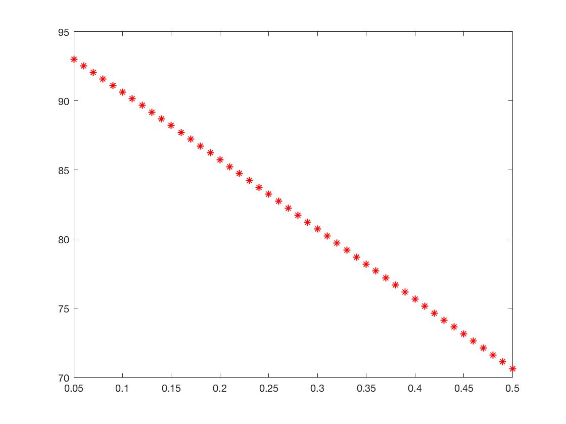
The bond price is decreasing in volatility, $\sigma$ , for log-normal jumps process.

Proof.

Mathematically,

	$\displaystyle\dfrac{\partial C_{J}(V_{t},D,\tau,\sigma^{2},r,\delta^{2},\lambda,k)}{\partial\sigma}$
	$\displaystyle=\dfrac{\partial}{\partial\sigma}(\sum^{\infty}_{n=0}\frac{(\lambda^{\prime}\tau)^{n}}{n!}e^{-\lambda^{\prime}\tau}C(V_{t},D,\tau,\sigma_{n},r_{n}))$
	$\displaystyle=\sum^{\infty}_{n=0}\frac{(\lambda^{\prime}\tau)^{n}}{n!}e^{-\lambda^{\prime}\tau}\dfrac{\partial C(V_{t},D,\tau,\sigma_{n},r_{n})}{\partial\sigma_{n}}$
	$\displaystyle=\sum^{\infty}_{n=0}\frac{(\lambda^{\prime}\tau)^{n}}{n!}e^{-\lambda^{\prime}\tau}x\sqrt{\tau}n(d_{1n})$
	$\displaystyle=x\sqrt{\tau}\sum^{\infty}_{n=0}\frac{(\lambda^{\prime}\tau)^{n}}{n!}e^{-\lambda^{\prime}\tau}n(d_{1n})>0.$

Then, $\dfrac{\partial B_{t}}{\partial\sigma}=-\dfrac{\partial C_{J}(V_{t},D,\tau,\sigma^{2},r,\delta^{2},\lambda,k)}{\partial\sigma}<0$ .

∎

$\Box$

When the volatility goes up, $B_{t}$ must decrease because the sum of $S_{t}$ and $B_{t}$ remains unchanged, call price increases as $V_{t}$ is more fluctuable. (See Figure 3).

Proposition III.4

(i) The bond price is decreasing in risk-free interest rate $r$ for log-normal jumps process.

(ii) $\dfrac{\partial B_{t}}{\partial r}\in(-\tau De^{-(r-\lambda k)\tau},0)$ .

Proof.

Actually,

	$\displaystyle\dfrac{\partial C_{J}(V_{t},D,\tau,\sigma^{2},r,\delta^{2},\lambda,k)}{\partial r}$
	$\displaystyle=\dfrac{\partial}{\partial r}(\sum^{\infty}_{n=0}\frac{(\lambda^{\prime}\tau)^{n}}{n!}e^{-\lambda^{\prime}\tau}C(V_{t},D,\tau,\sigma_{n},r_{n}))$
	$\displaystyle=\sum^{\infty}_{n=0}\frac{(\lambda^{\prime}\tau)^{n}}{n!}e^{-\lambda^{\prime}\tau}\dfrac{\partial C(V_{t},D,\tau,\sigma_{n},r_{n})}{\partial r_{n}}$
	$\displaystyle=\sum^{\infty}_{n=0}\frac{(\lambda^{\prime}\tau)^{n}}{n!}e^{-\lambda^{\prime}\tau}\tau De^{-r_{n}\tau}N(d_{2n})$
	$\displaystyle=\tau De^{-(r-\lambda k)\tau}\sum^{\infty}_{n=0}\frac{(\lambda^{\prime}\tau)^{n}}{n!}e^{-n\gamma}N(d_{2n})$
	$\displaystyle\in(0,\tau De^{-(r-\lambda k)\tau}).$

Then, $\dfrac{\partial B_{t}}{\partial r}=-\dfrac{\partial C_{J}(V_{t},D,\tau,\sigma^{2},r,\delta^{2},\lambda,k)}{\partial r}\in(-\tau De^{-(r-\lambda k)\tau},0)$ .

∎

$\Box$

Since the call option increases as $r$ goes up, $B_{t}$ must decrease the money market looks more attractive.(See Figure 4).

Proposition III.5

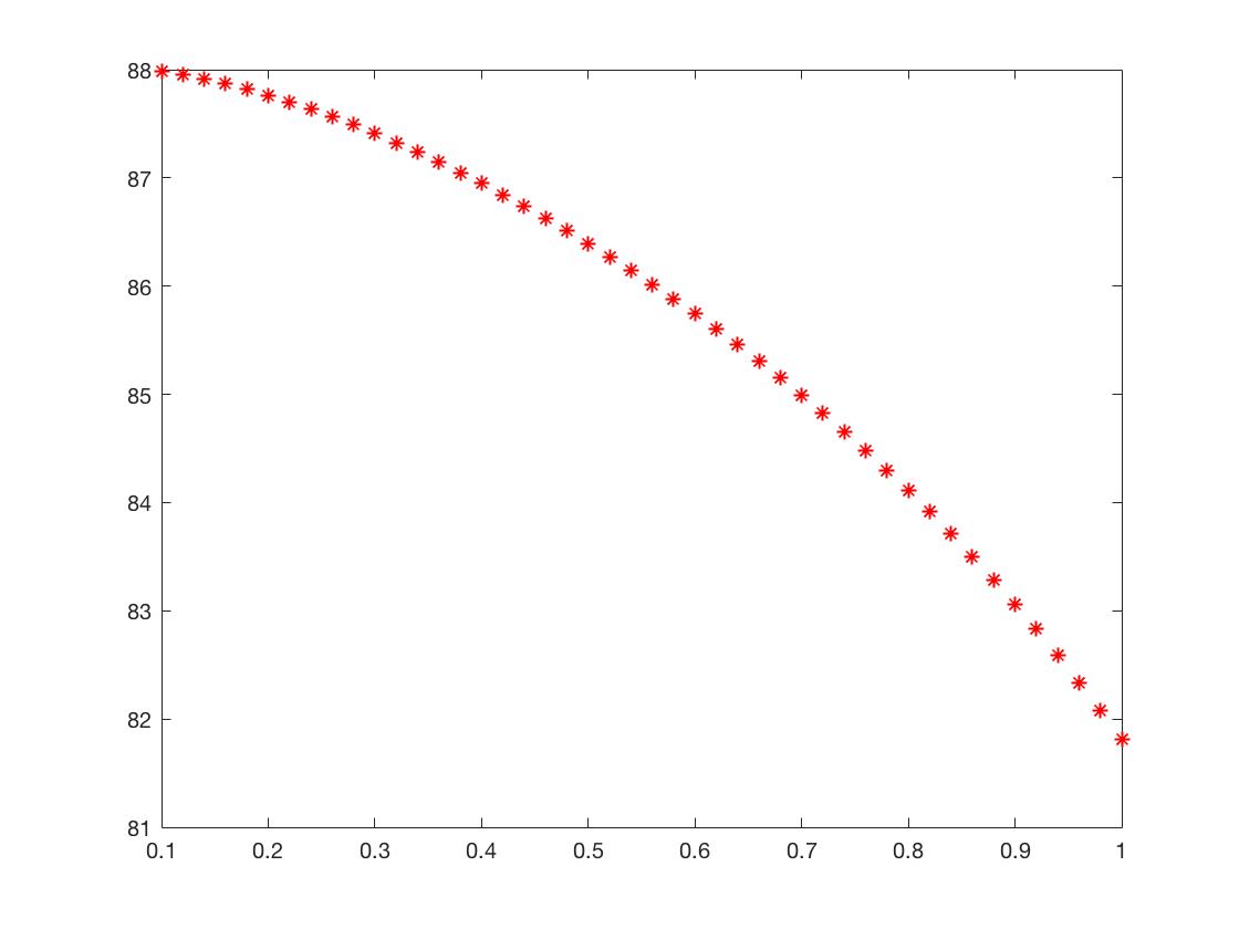
(i) The call price is increasing in time-to-maturity, $\tau$ , for the log-normal jumps process if $r-\lambda k\geq 0$ .

(ii) The bond price is decreasing in time-to-maturity, $\tau$ , for the log-normal jumps process $r-\lambda k\geq 0$ .

Proof.

See details at Appendix part 1.

We have $\frac{\partial B_{t}}{\partial k}<0$ . $B_{t}$ is decreasing due to the value of call increases when time-to-maturity is bigger.

In some extreme case, when $S_{2}$ is very small as a negative number, the sum of $S_{1}$ and $S_{2}$ can be negative which causes the tendency of $B_{t}$ w.r.t. $\tau$ is not decreasing.

∎

$\Box$

These two illustrations are listed as figure 5 and figure 6.

Proposition III.6

The bond price is decreasing in $\delta$ for the log-normal jumps process.

Proof.

We have

	$\displaystyle\dfrac{\partial C_{J}(V_{t},D,\tau,\sigma^{2},r,\delta^{2},\lambda,k)}{\partial\delta}$
	$\displaystyle=\dfrac{\partial}{\partial\delta}(\sum^{\infty}_{n=0}\frac{(\lambda^{\prime}\tau)^{n}}{n!}e^{-\lambda^{\prime}\tau}C(V_{t},D,\tau,\sigma_{n},r_{n}))$
	$\displaystyle=\sum^{\infty}_{n=0}\frac{(\lambda^{\prime}\tau)^{n}}{n!}e^{-\lambda^{\prime}\tau}\dfrac{\partial C(V_{t},D,\tau,\sigma_{n},r_{n}))}{\partial\sigma_{n}}\dfrac{\partial\sigma_{n}}{\partial\delta}$
	$\displaystyle=\sum^{\infty}_{n=0}\frac{(\lambda^{\prime}\tau)^{n}}{n!}e^{-\lambda^{\prime}\tau}x\sqrt{\tau}n(d_{1n})\frac{2n\delta}{\tau}$
	$\displaystyle=\frac{2x\delta}{\sqrt{\tau}}\sum^{\infty}_{n=0}\frac{(\lambda^{\prime}\tau)^{n}}{n!}e^{-\lambda^{\prime}\tau}n(d_{1n})n>0.$

Then, $\dfrac{\partial B_{t}}{\partial\delta}=-\dfrac{\partial C_{J}(V_{t},D,\tau,\sigma^{2},r,\delta^{2},\lambda,k)}{\partial\delta}<0$ .

∎

$\Box$

See Figure 7 for the simulation.

Proposition III.7

The bond price is decreasing in $\lambda$ for the log-normal jumps process.

Proof.

See details at Appendix part 2. Finally,

$\frac{\partial B_{t}}{\partial\lambda}<0$ holds.

∎

$\Box$

In fact, since $\lambda$ is the intensity of Poisson process, $\lambda$ increasing means the jump rate is bigger, the fluctuation will make the call price go up, so the bond price is decreasing accordingly. (See Figure 8)

Proposition III.8

The bond price is decreasing in $k$ for the log-normal jumps process.

Proof.

See details at Appendix part 3.

The result is $\frac{\partial B_{t}}{\partial k}<0$ .

∎

$\Box$

IV Conclusion

In this paper, we analytically explored the parameter sensitivities of bond price driven by compound Poisson process with log-normal distributed jumps. Meanwhile, we disclosed the corresponding interval of the sensitivities if available. Generally, the bond price in this case is increasing with respect to asset value $V_{t}$ and face value $D$ , decreasing with respect to volatility $\sigma$ , risk-free interest rate $r$ , log-normal standard deviation $\delta$ , Poisson intensity $\lambda$ and jumps’ mean $k$ . For the time-to-maturity $\tau$ , it is decreasing when $r-\lambda k\geq 0$ and undetermined for other cases.

Appendix

1. Proof of Proposition III.5

(i) The call price is increasing in time-to-maturity, $\tau$ , for the log-normal jumps process if $r-\lambda k\geq 0$ .

(ii) The bond price is decreasing in time-to-maturity, $\tau$ , for the log-normal jumps process $r-\lambda k\geq 0$ .

Proof.

	$\displaystyle\dfrac{\partial C^{J}(V_{t},D,\tau,\sigma^{2},r,\delta^{2},\lambda,k)}{\partial\tau}$
	$\displaystyle=\dfrac{\partial}{\partial\tau}(\sum^{\infty}_{n=0}\frac{(\lambda^{\prime}\tau)^{n}}{n!}e^{-\lambda^{\prime}\tau}C(V_{t},D,\tau,\sigma_{n},r_{n}))$
	$\displaystyle=\sum^{\infty}_{n=1}[n(\lambda^{\prime}\tau)^{n-1}\frac{\lambda^{\prime}}{n!}e^{-\lambda^{\prime}\tau}C_{n}(V_{t},D,\tau,\sigma_{n},r_{n})]$
	$\displaystyle\quad+\sum^{\infty}_{n=0}[\frac{(\lambda^{\prime}\tau)^{n}}{n!}(-\lambda^{\prime})e^{-\lambda^{\prime}\tau}C_{n}(V_{t},D,\tau,\sigma_{n},r_{n})]$
	$\displaystyle\quad+\sum^{\infty}_{n=0}[\frac{(\lambda^{\prime}\tau)^{n}}{n!}e^{-\lambda^{\prime}\tau}(\frac{\partial C(V_{t},D,\tau,\sigma_{n},r_{n})}{\partial\tau}$
	$\displaystyle\quad+\frac{\partial C(V_{t},D,\tau,\sigma_{n},r_{n})}{\partial r_{n}}\frac{\partial r_{n}}{\partial\tau}$
	$\displaystyle\quad+\frac{\partial C(V_{t},D,\tau,\sigma_{n},r_{n})}{\partial\tau}\frac{\partial\sigma_{n}}{\partial\tau})]$
	$\displaystyle=\sum^{\infty}_{n=1}[\frac{(\lambda^{\prime}\tau)^{n-1}}{(n-1)!}\lambda^{\prime}e^{-\lambda^{\prime}\tau}C_{n}(V_{t},D,\tau,\sigma_{n},r_{n})]$
	$\displaystyle\quad+\sum^{\infty}_{n=0}[\frac{(\lambda^{\prime}\tau)^{n}}{n!}(-\lambda^{\prime})e^{-\lambda^{\prime}\tau}C_{n}(V_{t},D,\tau,\sigma_{n},r_{n})]$
	$\displaystyle\quad+\sum^{\infty}_{n=0}[\frac{(\lambda^{\prime}\tau)^{n}}{n!}e^{-\lambda^{\prime}\tau}(\frac{\partial C(V_{t},D,\tau,\sigma_{n},r_{n})}{\partial\tau}$
	$\displaystyle\quad+\frac{\partial C(V_{t},D,\tau,\sigma_{n},r_{n})}{\partial r_{n}}\frac{\partial r_{n}}{\partial\tau}$
	$\displaystyle\quad+\frac{\partial C(V_{t},D,\tau,\sigma_{n},r_{n})}{\partial\tau}\frac{\partial\sigma_{n}}{\partial\tau})]$
	$\displaystyle=\sum^{\infty}_{n=0}[\frac{(\lambda^{\prime}\tau)^{n}}{n!}\lambda^{\prime}e^{-\lambda^{\prime}\tau}(C_{n+1}(V_{t},D,\tau,\sigma_{n},r_{n})$
	$\displaystyle\quad-C_{n}(V_{t},D,\tau,\sigma_{n},r_{n}))]$
	$\displaystyle\quad+\sum^{\infty}_{n=0}[\frac{(\lambda^{\prime}\tau)^{n}}{n!}e^{-\lambda^{\prime}\tau}(\frac{\partial C(V_{t},D,\tau,\sigma_{n},r_{n})}{\partial\tau}$
	$\displaystyle\quad+\frac{\partial C(V_{t},D,\tau,\sigma_{n},r_{n})}{\partial r_{n}}\frac{\partial r_{n}}{\partial\tau}$
	$\displaystyle\quad+\frac{\partial C(V_{t},D,\tau,\sigma_{n},r_{n})}{\partial\tau}\frac{\partial\sigma_{n}}{\partial\tau})]$
	$\displaystyle=S_{1}+S_{2},$

Separately, we consider the 1st part $S_{1}$ and 2nd part $S_{2}$ .

For $S_{1}$ , since

	$\displaystyle\dfrac{\partial C(V_{t},D,\tau,\sigma_{n},r_{n})}{\partial n}$
	$\displaystyle=xN^{\prime}(d_{1n})\dfrac{\partial d_{1n}}{\partial n}-De^{-r_{n}\tau}(-\dfrac{\partial r_{n}}{\partial n})\tau N(d_{2n})$
	$\displaystyle\quad+De^{-r_{n}\tau}N^{\prime}(d_{2n})\dfrac{\partial d_{2n}}{\partial n}$
	$\displaystyle=xN^{\prime}(d_{1n})(\dfrac{\partial d_{1n}}{\partial n}-\dfrac{\partial d_{2n}}{\partial n})+De^{-r_{n}\tau}\gamma\tau N(d_{2n})$
	$\displaystyle>0$

Where we used the facts:

	$\displaystyle xN^{\prime}(d_{1n})=Ke^{-r_{n}\tau}N^{\prime}(d_{2n}),$
	$\displaystyle d_{1n}-d_{2n}=\sigma_{n}\sqrt{\tau}\Rightarrow\dfrac{\partial d_{1n}}{\partial n}-\dfrac{\partial d_{2n}}{\partial n}=\frac{1}{2\sqrt{\sigma_{n}}}\dfrac{\delta^{2}}{\tau}\sqrt{\tau}>0.$

That means the function $C(V_{t},D,\tau,\sigma_{n},r_{n})$ is increasing w.r.t. $n$ , such that $S_{1}$ part is positive.

For $S_{2}$ , we taking partial derivative of $C(V_{t},D,\tau,\sigma_{n},r_{n})$ w.r.t. $\tau$ ,

	$\displaystyle S_{2}=\frac{\partial C(V_{t},D,\tau,\sigma_{n},r_{n})}{\partial\tau}+\frac{\partial C(V_{t},D,\tau,\sigma_{n},r_{n})}{\partial r_{n}}\frac{\partial r_{n}}{\partial\tau}$
	$\displaystyle\quad+\frac{\partial C(V_{t},D,\tau,\sigma_{n},r_{n})}{\partial\tau}\frac{\partial\sigma_{n}}{\partial\tau}$
	$\displaystyle=\frac{x\sigma_{n}}{2\sqrt{\tau}}n(d_{1n})+Dr_{n}e^{-r_{n}\tau}N(d_{2n})$
	$\displaystyle\quad+\tau De^{-r_{n}\tau}N(d_{2n})[n\gamma(-\tau^{-2})]$
	$\displaystyle\quad+x\sqrt{\tau}n(d_{1n})[\frac{1}{2}(\sigma_{n}^{2})^{-\frac{1}{2}}n\delta^{2}(-\tau^{-2})]$
	$\displaystyle=\frac{1}{2\sqrt{\tau}}xn(d_{1n})\frac{\sigma_{n}^{2}\tau-n\delta^{2}}{\sigma_{n}\tau}+De^{-r_{n}\tau}N(d_{2n})\frac{r_{n}\tau-n\gamma}{\tau}$
	$\displaystyle=\frac{1}{2\sqrt{\tau}}xn(d_{1n})\frac{\sigma^{2}}{\sigma_{n}}+De^{-r_{n}\tau}N(d_{2n})(r-\lambda k).$

here $r-\lambda k$ is non-negative as the condition, then $S_{2}$ is also positive, such that the initial $\frac{\partial C_{J}(V_{t},D,\tau,\sigma^{2},r,\delta^{2},\lambda,k)}{\partial\tau}$ is positive.

Hence $\frac{\partial B_{t}}{\partial k}=-\frac{\partial C_{J}(V_{t},D,\tau,\sigma^{2},r,\delta^{2},\lambda,k)}{\partial k}<0$ . $B_{t}$ is decreasing due to the value of call increases when time-to-maturity is bigger.

In some extreme case, when $S_{2}$ is very small as a negative number, the sum of $S_{1}$ and $S_{2}$ can be negative which causes the tendency of $B_{t}$ w.r.t. $\tau$ is not decreasing.

∎

$\Box$

2. Proof of Proposition III.7

The bond price is decreasing in $\lambda$ for the log-normal jumps process.

Proof.

Firstly, we can get that the call price is increasing in $\lambda$ .

Take partial derivative with respect to $\lambda$ in formula Merton ,

	$\displaystyle\frac{\partial C_{J}(V_{t},D,\tau,\sigma^{2},r,\delta^{2},\lambda,k)}{\partial\lambda}$
	$\displaystyle=\sum^{\infty}_{n=1}[n(\lambda^{\prime}\tau)^{n-1}(1+\beta)\frac{\tau}{n!}e^{-\lambda^{\prime}\tau}C(V_{t},D,\tau,\sigma_{n},r_{n})]$
	$\displaystyle\quad+\sum^{\infty}_{n=0}[\frac{(\lambda^{\prime}\tau)^{n}}{n!}(-\tau)(1+\beta)e^{-\lambda^{\prime}\tau}C(V_{t},D,\tau,\sigma_{n},r_{n})]$
	$\displaystyle\quad+\sum^{\infty}_{n=0}[\frac{(\lambda^{\prime}\tau)^{n}}{n!}e^{-\lambda^{\prime}\tau}\frac{\partial C(V_{t},D,\tau,\sigma_{n},r_{n})}{\partial\lambda}]$
	$\displaystyle=\sum^{\infty}_{n=1}[\frac{n}{\lambda}\frac{(\lambda^{\prime}\tau)^{n}}{(n)!}e^{-\lambda^{\prime}\tau)}C(V_{t},D,\tau,\sigma_{n},r_{n})]$
	$\displaystyle\quad+\sum^{\infty}_{n=0}[\frac{(\lambda^{\prime}\tau)^{n}}{n!}(-\tau)(1+\beta)e^{-\lambda^{\prime}\tau}C(V_{t},D,\tau,\sigma_{n},r_{n})]$
	$\displaystyle\quad+\sum^{\infty}_{n=0}[\frac{(\lambda^{\prime}\tau)^{n}}{n!}e^{-\lambda^{\prime}\tau}\frac{\partial C(V_{t},D,\tau,\sigma_{n},r_{n})}{\partial\lambda}]$
	$\displaystyle=\sum^{\infty}_{n=1}[\frac{(\lambda^{\prime}\tau)^{n}}{n!}e^{-\lambda^{\prime}\tau}C(V_{t},D,\tau,\sigma_{n},r_{n})(\frac{n}{\lambda}-(1+\beta)\tau)]$
	$\displaystyle\quad+(-\tau)(1+\beta)e^{-\lambda^{\prime}\tau}C_{0}(V,\tau,r_{n},\sigma_{n})$
	$\displaystyle\quad+\sum^{\infty}_{n=0}[\frac{(\lambda^{\prime}\tau)^{n}}{n!}e^{-\lambda^{\prime}\tau}(xN^{\prime}(d_{1n})\frac{\partial d_{1n}}{\partial r_{n}}(-\beta)$
	$\displaystyle\quad-Ke^{-r_{n}\tau}(-\tau)(-\beta)N(d_{2n})$
	$\displaystyle\quad-Ke^{-r_{n}\tau}N^{\prime}(d_{2n})\frac{\partial d_{2n}}{\partial r_{n}}(-\beta))]$
	$\displaystyle=\sum^{\infty}_{n=1}[\frac{(\lambda^{\prime}\tau)^{n}}{n!}e^{-\lambda^{\prime}\tau}C(V_{t},D,\tau,\sigma_{n},r_{n})(\frac{n}{\lambda}-(1+\beta)\tau)]$
	$\displaystyle\quad+(-\tau)(1+\beta)e^{-\lambda^{\prime}\tau}C_{0}(V,\tau,r_{n},\sigma_{n})$
	$\displaystyle\quad+\sum^{\infty}_{n=0}[\frac{(\lambda^{\prime}\tau)^{n}}{n!}e^{-\lambda^{\prime}\tau}(-Ke^{-r_{n}\tau}\tau\beta N(d_{2n}))]$
	$\displaystyle=\sum^{\infty}_{n=1}[\frac{(\lambda^{\prime}\tau)^{n}}{n!}e^{-\lambda^{\prime}\tau}C_{n}(V,\tau,r_{n},\sigma_{n})(\frac{n}{\lambda}-\tau-\beta\tau$
	$\displaystyle\quad+\beta\tau\frac{-Ke^{-r_{n}\tau}N(d_{2n})}{C_{n}(V,\tau,r_{n},\sigma_{n})})]-e^{-\lambda^{\prime}\tau}Ke^{-r_{0}\tau}\tau\beta N(d_{20})$
	$\displaystyle\quad-\tau(1+\beta)e^{-\lambda^{\prime}\tau}C_{0}(V,\tau,r_{n},\sigma_{n})$

	$\displaystyle=\sum^{\infty}_{n=1}[\frac{(\lambda^{\prime}\tau)^{n}}{n!}e^{-\lambda^{\prime}\tau}C_{n}(V,\tau,r_{n},\sigma_{n})(\frac{n}{\lambda}-\tau$
	$\displaystyle\quad-\beta\tau\frac{xN(d_{1n})}{C_{n}(V,\tau,r_{n},\sigma_{n})})]$
	$\displaystyle\quad-e^{-\lambda^{\prime}\tau}\tau(C_{0}(V_{t},D,\tau,\sigma_{n},r_{n})+\beta xN(d_{10}))$
	$\displaystyle=\sum^{\infty}_{n=0}[\frac{(\lambda^{\prime}\tau)^{n}}{n!}e^{-\lambda^{\prime}\tau}C_{n}(V,\tau,r_{n},\sigma_{n})(\frac{n}{\lambda}-\tau$
	$\displaystyle\quad-\beta\tau\frac{xN(d_{1n})}{C_{n}(V,\tau,r_{n},\sigma_{n})})]$

where we used the fact that

	$\displaystyle\frac{\partial d_{1}}{\partial r_{n}}=\frac{\partial d_{2}}{\partial r_{n}},$
	$\displaystyle xN^{\prime}(d_{1n})=Ke^{-r_{n}\tau}N^{\prime}(d_{2n}),$
	$\displaystyle C_{n}(V,\tau,r_{n},\sigma_{n})=xN(d_{1n})-Ke^{-r_{n}\tau}N(d_{2n}).$

Since $n$ can be a very large number in the sum, then the term $\frac{n}{\lambda}-\tau-\beta\tau\frac{xN(d_{1n})}{C_{n}}$ is positive for most cases. That means the partial derivative w.r.t. $\lambda$ is positive. So the call price is increasing against $\lambda$ .

We know $\frac{\partial C_{J}(V_{t},D,\tau,\sigma^{2},r,\delta^{2},\lambda,k)}{\partial\lambda}>0.$ Therefore, $\frac{\partial B_{t}}{\partial\lambda}=-\frac{\partial C_{J}(V_{t},D,\tau,\sigma^{2},r,\delta^{2},\lambda,k)}{\partial\lambda}<0$ holds.

∎

$\Box$

3. Proof of Proposition III.8

The bond price is decreasing in $k$ for the log-normal jumps process.

Proof.

Since

	$\displaystyle\dfrac{\partial C_{J}(V_{t},D,\tau,\sigma^{2},r,\delta^{2},\lambda,k)}{\partial k}$
	$\displaystyle=\dfrac{\partial}{\partial k}(\sum^{\infty}_{n=0}\frac{(\lambda^{\prime}\tau)^{n}}{n!}e^{-\lambda^{\prime}\tau}C_{n}(V_{t},D,\tau,\sigma_{n},r_{n}))$
	$\displaystyle=\sum^{\infty}_{n=1}[n(\lambda^{\prime}\tau)^{n-1}\frac{\lambda\tau}{n!}e^{-\lambda^{\prime}\tau}C_{n}(V_{t},D,\tau,\sigma_{n},r_{n})]$
	$\displaystyle\quad+\sum^{\infty}_{n=0}[\frac{(\lambda^{\prime}\tau)^{n}}{n!}(-\tau\lambda)e^{-\lambda^{\prime}\tau}C_{n}(V_{t},D,\tau,\sigma_{n},r_{n})]$
	$\displaystyle\quad+\sum^{\infty}_{n=0}[\frac{(\lambda^{\prime}\tau)^{n}}{n!}e^{-\lambda^{\prime}\tau}\frac{\partial C_{n}(V_{t},D,\tau,\sigma_{n},r_{n})}{\partial k}]$
	$\displaystyle=\sum^{\infty}_{n=1}[\frac{n}{1+k}\frac{(\lambda^{\prime}\tau)^{n}}{(n)!}e^{-\lambda^{\prime}\tau)}C_{n}(V_{t},D,\tau,\sigma_{n},r_{n})]$
	$\displaystyle\quad+\sum^{\infty}_{n=0}[\frac{(\lambda^{\prime}\tau)^{n}}{n!}(-\lambda\tau)e^{-\lambda^{\prime}\tau}C_{n}(V_{t},D,\tau,\sigma_{n},r_{n})]$

	$\displaystyle\quad+\sum^{\infty}_{n=0}[\frac{(\lambda^{\prime}\tau)^{n}}{n!}e^{-\lambda^{\prime}\tau}\frac{\partial C_{n}(V_{t},D,\tau,\sigma_{n},r_{n})}{\partial k}]$
	$\displaystyle=\sum^{\infty}_{n=1}[\frac{(\lambda^{\prime}\tau)^{n}}{n!}e^{-\lambda^{\prime}\tau}C_{n}(V_{t},D,\tau,\sigma_{n},r_{n})(\frac{n}{1+k}-\lambda\tau)]$
	$\displaystyle\quad+(-\lambda\tau)e^{-\lambda^{\prime}\tau}C_{0}(V_{t},D,\tau,\sigma_{n},r_{n})$
	$\displaystyle\quad+\sum^{\infty}_{n=0}[\frac{(\lambda^{\prime}\tau)^{n}}{n!}e^{-\lambda^{\prime}\tau}(xN^{\prime}(d_{1n})\frac{\partial d_{1n}}{\partial r_{n}}(\frac{n}{(1+k)\tau}-\lambda)$
	$\displaystyle\quad-De^{-r_{n}\tau}(-\tau)(\frac{n}{(1+k)\tau}-\lambda)N(d_{2n})$
	$\displaystyle\quad-De^{-r_{n}\tau}N^{\prime}(d_{2n})\frac{\partial d_{2n}}{\partial r_{n}}(\frac{n}{(1+k)\tau}-\lambda))]$
	$\displaystyle=\sum^{\infty}_{n=1}[\frac{(\lambda^{\prime}\tau)^{n}}{n!}e^{-\lambda^{\prime}\tau}C_{n}(V_{t},D,\tau,\sigma_{n},r_{n})(\frac{n}{1+k}-\lambda\tau)]$
	$\displaystyle\quad+(-\lambda\tau)e^{-\lambda^{\prime}\tau}C_{0}(V_{t},D,\tau,\sigma_{n},r_{n})$
	$\displaystyle\quad+\sum^{\infty}_{n=0}[\frac{(\lambda^{\prime}\tau)^{n}}{n!}e^{-\lambda^{\prime}\tau}(De^{-r_{n}\tau}(\frac{n}{1+k}-\lambda\tau)N(d_{2n}))]$
	$\displaystyle=\sum^{\infty}_{n=1}[\frac{(\lambda^{\prime}\tau)^{n}}{n!}e^{-\lambda^{\prime}\tau}C_{n}(V_{t},D,\tau,\sigma_{n},r_{n})(\frac{n-\lambda^{\prime}\tau}{1+k})$
	$\displaystyle\quad\frac{C_{n}(V_{t},D,\tau,\sigma_{n},r_{n})+De^{-r_{n}\tau}N(d_{2n})}{C_{n}(V_{t},D,\tau,\sigma_{n},r_{n})})]$
	$\displaystyle\quad-\lambda\tau e^{-\lambda^{\prime}\tau}C_{0}(V_{t},D,\tau,\sigma_{n},r_{n})-e^{-\lambda^{\prime}\tau}De^{-r_{0}\tau}\lambda\tau N(d_{20})$

	$\displaystyle=\sum^{\infty}_{n=1}[\frac{(\lambda^{\prime}\tau)^{n}}{n!}e^{-\lambda^{\prime}\tau}(\frac{n-\lambda^{\prime}\tau}{1+k})xN(d_{1n}))]$
	$\displaystyle\quad-e^{-\lambda^{\prime}\tau}\lambda\tau(C_{0}(V_{t},D,\tau,\sigma_{n},r_{n})+De^{-r_{0}\tau}N(d_{20}))$
	$\displaystyle=\sum^{\infty}_{n=1}[\frac{(\lambda^{\prime}\tau)^{n}}{n!}e^{-\lambda^{\prime}\tau}(\frac{n-\lambda^{\prime}\tau}{1+k})xN(d_{1n})]-e^{-\lambda^{\prime}\tau}\lambda\tau xN(d_{10})$
	$\displaystyle=\sum^{\infty}_{n=0}[\frac{(\lambda^{\prime}\tau)^{n}}{n!}e^{-\lambda^{\prime}\tau}(\frac{n-\lambda^{\prime}\tau}{1+k})xN(d_{1n})].$

where we used the fact that

	$\displaystyle\frac{\partial d_{1}}{\partial r_{n}}=\frac{\partial d_{2}}{\partial r_{n}},$
	$\displaystyle xN^{\prime}(d_{1n})=De^{-r_{n}\tau}N^{\prime}(d_{2n}),$
	$\displaystyle C_{n}(V_{t},D,\tau,\sigma_{n},r_{n})=xN(d_{1n})-De^{-r_{n}\tau}N(d_{2n}).$

Since $n$ goes to larger and large in the sum, then the term $\frac{n-\lambda^{\prime}\tau}{1+k}$ is positive for most cases. That means the partial derivative w.r.t. $k$ is positive. Then, $\frac{\partial B_{t}}{\partial k}=-\frac{\partial C_{J}}{\partial k}<0$ .

∎

$\Box$

References

(1) Black, Fischer and Myron Scholes (1973), The Pricing of Options and Corporate Liabilities Journal of Political Economy, 81, 637-659.
(2) Merton, R. C. (1976), Option pricing when underlying stock returns are discontinuous., J. Financial Economy. 3 125–144.
(3) Steven Shreve, (2010), Stochastic Calculus for Finance II: Continuous-Time Models, Springer.
(4) David Lando, (2004), Credit Risk Modeling: Theory and Applications, Princeton University Press.
(5) Chunsheng Zhou, A Jump-Diffusion Approach to Modeling Credit Risk and Valuing Defaultable Securities, Finance and Economics Discussion Series 1997-15 / Board of Governors of the Federal Reserve System, 1997.
(6) Hull, J. C. (2003). Options futures and other derivatives. Pearson Education India.
(7) Scott, Louis (1997), Pricing Stock Options in a Jump-Diffusion Model with Stochastic Volatility and Interest Rates: Application of Fourier Inversion Methods Mathematical Finance, 7, 413-426.
(8) Camara, Antonio and Li, Weiping, Jump-Diffusion Option Pricing without IID Jumps Available at SSRN: https://ssrn.com/abstract=1282882 or http://dx.doi.org/10.2139/ssrn.1282882
(9) Bates, David (1996), Jumps and Stochastic Volatility: Exchange Rate Processes Implicit in Deutschemark Options Review of Financial Studies, 9, 69-108.
(10) Hirsa, Ali, (2011), Computational Methods in Finance Chapman&Hull/CRC.
(11) Kienitz, J., Wetterau, D. (2012), Financial Modelling: Theory, Implementation and Practice with MATLAB Source Wiley Finance, Chichester..
(12) N. Cai and S. Kou. Pricing Asian options under a hyper-exponential jump diffusion model. Oper. Res., 60(1):64–77, 2012.
(13) S. Kou. A jump-diffusion model for option pricing. Management Sci., 48(8):1086–1101, 2002.