The original Weyl-Titchmarsh functions and sectorial Schrödinger L-systems
Abstract.
In this paper we study the L-system realizations generated by the original Weyl-Titchmarsh functions in the case when the minimal symmetric Schrödinger operator in is non-negative. We realize functions as impedance functions of Schrödinger L-systems and derive necessary and sufficient conditions for to fall into sectorial classes of Stieltjes functions. Moreover, it is shown that the knowledge of the value and parameter allows us to describe the geometric structure of the L-system that realizes . Conditions when the main and state space operators of the L-system realizing have the same or not angle of sectoriality are presented in terms of the parameter . Example that illustrates the obtained results is presented in the end of the paper.
Key words and phrases:
L-system, Schrödinger operator, transfer function, impedance function, Herglotz-Nevanlinna function, Stieltjes function, Weyl-Titchmarsh function1991 Mathematics Subject Classification:
Primary 47A10; Secondary 47N50, 81Q101. Introduction
This paper is a part of an ongoing project studying the realizations of the original Weyl-Titchmarsh function and its linear-fractional transformation associated with a Schrödinger operator in . In this project the Herglotz-Nevanlinna functions and as well as and are being realized as impedance functions of L-systems with a dissipative Schrödinger main operator , (). For the sake of brevity we will refer to these L-systems as Schrödinger L-systems for the rest of the manuscript. The formal definition, exposition and discussions of general and Schrödinger L-systems are presented in Sections 2 and 4. We capitalize on the fact that all Schrödinger L-systems form a two-parametric family whose members are uniquely defined by a real-valued parameter and a complex boundary value of the main dissipative operator.
The focus of this paper is set on the case when the realizing Schrödinger L-systems are based on non-negative symmetric Schrödinger operator with deficiency indices and have accretive state-space operator. It is known (see [2]) that in this case the impedance functions of such L-systems are Stieltjes. Here we study the situation when the realizing Schrödinger L-systems are also sectorial and the Weyl-Titchmarsh functions fall into sectorial classes and of Stieltjes functions that are discussed in details in Section 3. Section 5 provides us with the general realization results (obtained in [7]) for the functions , , and . It is shown that , , and can be realized as the impedance function of Schrödinger L-systems , , and , respectively.
The main results of the paper are contained in Section 6. Here we apply the realization theorems from Section 5 to Schrödinger L-systems that are based on non-negative symmetric Schrödinger operator to obtain additional properties. Utilizing the results presented in Section 4, we derive some new features of Schrödinger L-systems whose impedance functions fall into particular sectorial classes with and explicitly described. The results are given in terms of the parameter that appears in the definition of the function . Moreover, the knowledge of the limit value and the value of allows us to find the angle of sectoriality of the main and state-space operators of the realizing L-system. This, in turn, leads to connections to Kato’s problem about sectorial extension of sectorial forms.
The paper is concluded with an example that illustrates main results and concepts. The present work is a further development of the theory of open physical systems conceived by M. Livs̆ic in [19].
2. Preliminaries
For a pair of Hilbert spaces , we denote by the set of all bounded linear operators from to . Let be a closed, densely defined, symmetric operator in a Hilbert space with inner product . Any non-symmetric operator in such that is called a quasi-self-adjoint extension of .
Consider the rigged Hilbert space (see [11], [2]) where and
| (1) |
Let be the Riesz-Berezansky operator (see [11], [2]) which maps onto such that (, ) and . Note that identifying the space conjugate to with , we get that if , then An operator is called a self-adjoint bi-extension of a symmetric operator if and . Let be a self-adjoint bi-extension of and let the operator in be defined as follows:
The operator is called a quasi-kernel of a self-adjoint bi-extension (see [26], [2, Section 2.1]). A self-adjoint bi-extension of a symmetric operator is called t-self-adjoint (see [2, Definition 4.3.1]) if its quasi-kernel is self-adjoint operator in . An operator is called a quasi-self-adjoint bi-extension of an operator if and We will be mostly interested in the following type of quasi-self-adjoint bi-extensions. Let be a quasi-self-adjoint extension of with nonempty resolvent set . A quasi-self-adjoint bi-extension of an operator is called (see [2, Definition 3.3.5]) a ()-extension of if is a t-self-adjoint bi-extension of . In what follows we assume that has deficiency indices . In this case it is known [2] that every quasi-self-adjoint extension of admits -extensions. The description of all -extensions via Riesz-Berezansky operator can be found in [2, Section 4.3].
Recall that a linear operator in a Hilbert space is called accretive [17] if for all . We call an accretive operator -sectorial [17] if there exists a value of such that
| (2) |
We say that the angle of sectoriality is exact for a -sectorial operator if
An accretive operator is called extremal accretive if it is not -sectorial for any . A -extension of is called accretive if for all . This is equivalent to that the real part is a nonnegative t-self-adjoint bi-extension of .
The following definition is a “lite” version of the definition of L-system given for a scattering L-system with one-dimensional input-output space. It is tailored for the case when the symmetric operator of an L-system has deficiency indices . The general definition of an L-system can be found in [2, Definition 6.3.4] (see also [10] for a non-canonical version).
Definition 1.
An array
| (3) |
is called an L-system if:
-
(1)
is a dissipative (, ) quasi-self-adjoint extension of a symmetric operator with deficiency indices ;
-
(2)
is a ()-extension of ;
-
(3)
, where and .
Operators and are called a main and state-space operators respectively of the system , and is a channel operator. It is easy to see that the operator of the system (3) is such that , and pick , (see [2]). A system in (3) is called minimal if the operator is a prime operator in , i.e., there exists no non-trivial reducing invariant subspace of on which it induces a self-adjoint operator. Minimal L-systems of the form (3) with one-dimensional input-output space were also considered in [6].
We associate with an L-system the function
| (4) |
which is called the transfer function of the L-system . We also consider the function
| (5) |
that is called the impedance function of an L-system of the form (3). The transfer function of the L-system and function of the form (5) are connected by the following relations valid for , ,
An L-system of the form (3) is called an accretive L-system ([9], [14]) if its state-space operator operator is accretive, that is for all . An accretive L-system is called sectorial if the operator is sectorial, i.e., satisfies (2) for some and all .
3. Sectorial classes and and their realizations
A scalar function is called the Herglotz-Nevanlinna function if it is holomorphic on , symmetric with respect to the real axis, i.e., , , and if it satisfies the positivity condition , . The class of all Herglotz-Nevanlinna functions, that can be realized as impedance functions of L-systems, and connections with Weyl-Titchmarsh functions can be found in [2], [6], [13], [15] and references therein. The following definition can be found in [16]. A scalar Herglotz-Nevanlinna function is a Stieltjes function if it is holomorphic in and
| (6) |
It is known [16] that a Stieltjes function admits the following integral representation
| (7) |
where and is a non-decreasing on function such that We are going to focus on the class (see [9], [14], [2]) of scalar Stieltjes functions such that the measure in representation (7) is of unbounded variation. It was shown in [2] (see also [9]) that such a function can be realized as the impedance function of an accretive L-system of the form (3) with a densely defined symmetric operator if and only if it belongs to the class .
Now we are going to consider sectorial subclasses of scalar Stieltjes functions introduced in [1]. Let . Sectorial subclasses of Stieltjes functions are defined as follows: a scalar Stieltjes function belongs to if
| (8) |
for an arbitrary sequences of complex numbers , () and , (). For , we have
where denotes the class of all Stieltjes functions (which corresponds to the case ). Let be a minimal L-system of the form (3) with a densely defined non-negative symmetric operator . Then (see [2]) the impedance function defined by (5) belongs to the class if and only if the operator of the L-system is -sectorial.
Let , , and . We say that a scalar Stieltjes function belongs to the class if
| (9) |
The following connection between the classes and can be found in [2]. Let be an L-system of the form (3) with a densely defined non-negative symmetric operator with deficiency numbers Let also be an -sectorial -extension of . Then the impedance function defined by (5) belongs to the class , . Moreover, the main operator is -sectorial with the exact angle of sectoriality . In the case when is the exact angle of sectoriality of the operator we have that (see [2]). It also follows that under this set of assumptions, the impedance function is such that in representation (7).
Now let be an L-system of the form (3), where is a -extension of and is a closed densely defined non-negative symmetric operator with deficiency numbers It was proved in [2] that if the impedance function belongs to the class and , then is -sectorial, where
| (10) |
Under the above set of conditions on L-system , it is shown in [2] that is -sectorial -extension of an -sectorial operator with the exact angle if and only if . Moreover, the angle can be found via the formula
| (11) |
where is the measure from integral representation (7) of .
4. L-systems with Schrödinger operator and their impedance functions
Let , , and , where is a real locally summable on function. Suppose that the symmetric operator
| (12) |
has deficiency indices (1,1). Let be the set of functions locally absolutely continuous together with their first derivatives such that . Consider with the scalar product
Let be the corresponding triplet of Hilbert spaces. Consider the operators
| (13) |
where . Let be a symmetric operator of the form (12) with deficiency indices (1,1), generated by the differential operation . Let also be the solutions of the following Cauchy problems:
It is well known [20], [18] that there exists a function introduced by H. Weyl [27], [28] for which
belongs to . The function is not a Herglotz-Nevanlinna function but and are.
Now we shall construct an L-system based on a non-self-adjoint Schrödinger operator with . It was shown in [4], [2] that the set of all ()-extensions of a non-self-adjoint Schrödinger operator of the form (13) in can be represented in the form
| (14) |
Moreover, the formulas (14) establish a one-to-one correspondence between the set of all ()-extensions of a Schrödinger operator of the form (13) and all real numbers . One can easily check that the ()-extension in (14) of the non-self-adjoint dissipative Schrödinger operator , () of the form (13) satisfies the condition
where
| (15) |
and are the delta-function and its derivative at the point , respectively. Furthermore,
where , , and is the triplet of Hilbert spaces discussed above.
It was also shown in [2] that the quasi-kernel of is given by
| (16) |
Let , . It is clear that
| (17) |
and Therefore, the array
| (18) |
is an L-system with the main operator , () of the form (13), the state-space operator of the form (14), and with the channel operator of the form (17). It was established in [4], [2] that the transfer and impedance functions of are
| (19) |
and
| (20) |
It was shown in [2, Section 10.2] that if the parameters and are related via (16), then the two L-systems and of the form (18) have the following property
| (21) |
5. Realizations of , and .
It is known [18], [20] that the original Weyl-Titchmarsh function has a property that is a Herglotz-Nevanlinna function. The question whether can be realized as the impedance function of a Schrödinger L-system is answered in the following theorem that was proved in [7].
Theorem 2 ([7]).
Let be a symmetric Schrödinger operator of the form (12) with deficiency indices and locally summable potential in If is the Weyl-Titchmarsh function of , then the Herglotz-Nevanlinna function can be realized as the impedance function of a Schrödinger L-system of the form (18) with and .
Conversely, let be a Schrödinger L-system of the form (18) with the symmetric operator such that for all and . Then the parameters and defining are such that and .
A similar result for the function was also proved in [7].
Theorem 3 ([7]).
Let be a symmetric Schrödinger operator of the form (12) with deficiency indices and locally summable potential in If is the Weyl-Titchmarsh function of , then the Herglotz-Nevanlinna function can be realized as the impedance function of a Schrödinger L-system of the form (18) with and .
Conversely, let be a Schrödinger L-system of the form (18) with the symmetric operator such that for all and . Then the parameters and defining are such that and .
Now we recall the definition of Weyl-Titchmarsh functions . Let be a symmetric operator of the form (12) with deficiency indices (1,1), generated by the differential operation . Let also and be the solutions of the following Cauchy problems:
It is known [12], [20], [21] that there exists an analytic in function for which
| (23) |
belongs to . It is easy to see that if , then . The functions and are connected (see [12], [21]) by
| (24) |
We know [20], [21] that for any real the function is a Herglotz-Nevanlinna function. Also, modifying (24) slightly we obtain
| (25) |
The following realization theorem (see [7]) for Herglotz-Nevanlinna functions is similar to Theorem 2.
Theorem 4 ([7]).
We note that when we obtain , , and the realizing Schrödinger L-system is thoroughly described in [7, Section 5]. If , then we get , , and the realizing Schrödinger L-system is (see [7, Section 5]). Assuming that and neither nor we give the description of a Schrödinger L-system realizing as follows.
| (27) |
where
| (28) |
, and
| (29) |
Also,
| (30) | ||||
6. Non-negative Schrödinger operator and sectorial L-systems
Now let us assume that is a non-negative (i.e., for all ) symmetric operator of the form (12) with deficiency indices (1,1), generated by the differential operation . The following theorem takes place.
Theorem 5 ([23], [24], [25]).
Let be a nonnegative symmetric Schrödinger operator of the form (12) with deficiency indices and locally summable potential in Consider operator of the form (13). Then
-
(1)
operator has more than one non-negative self-adjoint extension, i.e., the Friedrichs extension and the Kreĭn-von Neumann extension do not coincide, if and only if ;
-
(2)
operator , () coincides with the Kreĭn-von Neumann extension if and only if ;
-
(3)
operator is accretive if and only if
(31) -
(4)
operator , () is -sectorial if and only if holds;
-
(5)
operator , () is accretive but not -sectorial for any if and only if
-
(6)
If is -sectorial, then the exact angle can be calculated via
(32)
For the remainder of this paper we assume that . Then according to Theorem 5 above (see also [3], [22], [25]) we have the existence of the operator , () that is accretive and/or sectorial. It was shown in [2] that if is an accretive Schrödinger operator of the form (13), then for all real satisfying the following inequality
| (33) |
formulas (14) define the set of all accretive -extensions of the operator . Moreover, an accretive -extensions of a sectorial operator with exact angle of sectoriality also preserves the same exact angle of sectoriality if and only if in (14) (see [8, Theorem 3]). Also, is accretive but not -sectorial for any ()-extension of if and only if in (14)
| (34) |
(see [8, Theorem 4]). An accretive operator has a unique accretive -extension if and only if In this case this unique -extension has the form
| (35) | ||||
Now we are going to turn to functions described by (23)-(24) and associated with the non-negative operator above. We need to see how the parameter in the definition of affects the L-system realizing . This question was answered in [7, Theorem 6.3]. It tells us that if the non-negative symmetric Schrödinger operator is such that , then the L-system of the form (27) realizing the function is accretive if and only if
| (36) |
Note that if in (36), then and . Also, from [7, Theorem 6.2] we know that if , then is realized by an accretive system .
Now once we established a criteria for an L-system realizing to be accretive, we can look into more of its properties. There are two choices for an accretive L-system : it is either (1) accretive sectorial or (2) accretive extremal. In the case (1) we have that of the form (28) is -sectorial with some angle of sectoriality that can only exceed the exact angle of sectoriality of . In the case (2) the state-space operator is extremal (not sectorial for any ) and is a -extension of that itself can be either -sectorial or extremal. These possibilities were described in details in [7, Theorem 6.4]. In particular, it was shown that for the accretive L-system realizing the function the following is true:
-
(1)
if , then there is only one accretive L-system realizing . This L-system is extremal and its main operator is extremal as well.
-
(2)
if , then is -sectorial for and
-
(a)
if , then is extremal;
-
(b)
if , then is -sectorial with ;
-
(c)
if , then is -sectorial.
-
(a)
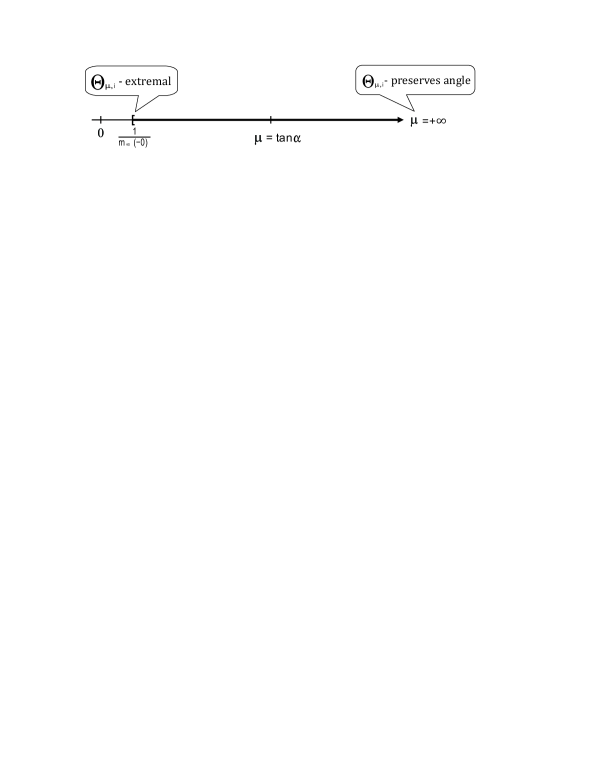
Figure 1 above describes the dependence of the properties of realizing L-systems on the value of and hence . The bold part of the real line depicts values of that produce accretive L-systems .
Additional analytic properties of the functions , , and were described in [7, Theorem 6.5]. It was proved there that under the current set of assumptions we have:
-
(1)
the function is Stieltjes if and only if ;
-
(2)
the function is never Stieltjes;111It will be shown in an upcoming paper that if , then the function is actually inverse Stieltjes.
-
(3)
the function given by (24) is Stieltjes if and only if
Now we are going to turn to the case when our realizing L-system is accretive sectorial. To begin with let be an L-system of the form (18), where is a ()-extension (14) of the accretive Schrödinger operator . Here we summarize and list some known facts about possible accretivity and sectoriality of .
- •
- •
-
•
is accretive but not -sectorial for any if and only if .
-
•
If is such that , then belongs to the class . In the case when we have (see [5]).
- •
-
•
If is -sectorial with the exact angle of sectoriality , then it admits only one -sectorial ()-extension with the same angle of sectoriality . Consequently, and has the form (35).
- •
Note that it follows from the above that any -sectorial operator with the exact angle of sectoriality admits only one accretive ()-extension that is not -sectorial for any . This extension takes form (14) with given by (34).
Now let us consider a function and Schrödinger L-system of the form (27) that realizes it. According to [7, Theorem 6.4-6.5] this L-system is sectorial if and only if
| (37) |
If we assume that L-system is -sectorial, then its impedance function belongs to certain sectorial classes discussed in Section 3. Namely, . The following theorem provides more refined properties of for this case.
Theorem 6.
Let be the accretive L-system of the form (27) realizing the function associated with the non-negative operator . Let also be a -sectorial -extension of defined by (22). Then the function belongs to the class , ,
| (38) |
and
| (39) |
Moreover, the operator is -sectorial with the exact angle of sectoriality .
Proof.
It is given that is -sectorial and hence (37) holds. For further convenience we re-write as
| (40) |
Since under our assumption is -sectorial, then its impedance function belongs to certain sectorial classes discussed in Section 3. Namely, and . In order to describe we take into account (see [2, Section 10.3]) that to obtain
In order to get we simply pass to the limit in (40)
The above confirms (38) and (39). In order to show the rest, we apply [2, Theorem 9.8.4]. This theorem states that if is a -sectorial -extension of a main operator of an L-system , then the impedance function belongs to the class , , and is -sectorial with the exact angle of sectoriality . It can also be checked directly that formulas (38) and (39) (under condition (37)) imply and hence the definition of -sectoriality applies correctly. ∎

Now we state and prove the following.
Theorem 7.
Proof.
We note first that the conditions of our theorem imply the following . Thus, according to [7, Theorem 6.4] part 2(c), a ()-extension is -sectorial for some . Then we can apply Theorem 6 to confirm that , where and are described by (38) and (39). The first part of formula (41) follows from [8, Theorem 8] applied to the L-system with (see also [2, Theorem 9.8.7]). Note that since is a -sectorial extension of a -sectorial operator , then with equality possible only when (see [2], [8]). Since we chose , then and hence that confirms the second part of formula (41).
7. Example
We conclude this paper with a simple illustration. Consider the differential expression with the Bessel potential
of order in the Hilbert space . The minimal symmetric operator
| (42) |
generated by this expression and boundary conditions has defect numbers . Let . It is known [2] that in this case
and The minimal symmetric operator then becomes
| (43) |
The main operator of the form (13) is written for as
| (44) |
will be shared by all the family of L-systems realizing functions described by (23)-(24). This operator is accretive and -sectorial since with the exact angle of sectoriality given by (see (32))
| (45) |
A family of L-systems of the form (27) that realizes functions described by (23)–(25) as
| (46) |
was constructed in [7]. According to [7, Theorem 6.3] the L-systems in (27) are accretive if
Using part (2c) of [7, Theorem 6.4], we get that the realizing L-system in (27) preserves the angle of sectoriality and becomes -sectorial if or . Therefore the L-system
| (47) |
where
| (48) |
, and realizes the function . Also,
| (49) | ||||
This L-system is clearly accretive according to [7, Theorem 6.2] which is also independently confirmed by direct evaluation
Moreover, according to [7, Theorem 6.4] (see also [2, Theorem 9.8.7]) the L-system is -sectorial. Taking into account that (see formula (15)) we obtain inequality (2) with , that is or
| (50) |
In addition, we have shown that the -sectorial form defined on can be extended to the -sectorial form defined on (see (43)–(44)) having the exact (for both forms) angle of sectoriality . A general problem of extending sectorial sesquilinear forms to sectorial ones was mentioned by T. Kato in [17]. It can be easily seen that function in (49) belongs to a sectorial class of Stieltjes functions.
References
- [1] D. Alpay, E. Tsekanovskiĭ, Interpolation theory in sectorial Stieltjes classes and explicit system solutions, Lin. Alg. Appl., 314, (2000), 91–136.
- [2] Yu. Arlinskiĭ, S. Belyi, E. Tsekanovskiĭ Conservative Realizations of Herglotz-Nevanlinna functions, Operator Theory: Advances and Applications, Vol. 217, Birkhauser Verlag, 2011.
- [3] Yu. Arlinskiĭ, E. Tsekanovskiĭ, M. Krein’s research on semi-bounded operators, its contemporary developments, and applications, Oper. Theory Adv. Appl., vol. 190, (2009), 65–112.
- [4] Yu. Arlinskiĭ, E. Tsekanovskiĭ, Linear systems with Schrödinger operators and their transfer functions, Oper. Theory Adv. Appl., 149, 2004, 47–77.
- [5] S. Belyi, Sectorial Stieltjes functions and their realizations by L-systems with Schrödinger operator, Mathematische Nachrichten, vol. 285, no. 14-15, (2012), pp. 1729-1740.
- [6] S. Belyi, K. A. Makarov, E. Tsekanovskiĭ, Conservative L-systems and the Livšic function. Methods of Functional Analysis and Topology, 21, no. 2, (2015), 104–133.
- [7] S. Belyi, E. Tsekanovskiĭ, On realization of the original Weyl-Titchmarsh functions by Schrödinger L-systems, Complex Analysis and Operator Theory, 15 (11), (2021).
- [8] S. Belyi, E. Tsekanovskiĭ, On Sectorial L-systems with Schrödinger operator, Differential Equations, Mathematical Physics, and Applications. Selim Grigorievich Krein Centennial, CONM, vol. 734, American Mathematical Society, Providence, RI (2019), 59-76.
- [9] S. Belyi, E. Tsekanovskiĭ, Stieltjes like functions and inverse problems for systems with Schrödinger operator. Operators and Matrices, vol. 2, No.2, (2008), 265–296.
- [10] S. Belyi, S. Hassi, H.S.V. de Snoo, E. Tsekanovskiĭ, A general realization theorem for matrix-valued Herglotz-Nevanlinna functions, Linear Algebra and Applications. vol. 419, (2006), 331–358.
- [11] Yu. Berezansky, Expansion in eigenfunctions of self-adjoint operators, vol. 17, Transl. Math. Monographs, AMS, Providence, 1968.
- [12] A.A. Danielyan, B.M. Levitan, On the asymptotic behaviour of the Titchmarsh-Weyl m-function, Izv. Akad. Nauk SSSR Ser. Mat., Vol. 54, Issue 3, (1990), 469–479.
- [13] V. Derkach, M.M. Malamud, E. Tsekanovskiĭ, Sectorial Extensions of Positive Operators. (Russian), Ukrainian Mat.J. 41, No.2, (1989), pp. 151–158.
- [14] I. Dovzhenko and E. Tsekanovskiĭ, Classes of Stieltjes operator-functions and their conservative realizations, Dokl. Akad. Nauk SSSR, 311 no. 1 (1990), 18–22.
- [15] F. Gesztesy, E. Tsekanovskiĭ, On Matrix-Valued Herglotz Functions. Math. Nachr. 218, (2000), 61–138.
- [16] I.S. Kac, M.G. Krein, -functions – analytic functions mapping the upper halfplane into itself, Amer. Math. Soc. Transl., Vol. 2, 103, 1-18, 1974.
- [17] T. Kato, Perturbation Theory for Linear Operators, Springer-Verlag, 1966.
- [18] B.M. Levitan, Inverse Sturm-Liouville problems. Translated from the Russian by O. Efimov. VSP, Zeist, (1987)
- [19] M.S. Livšic, Operators, oscillations, waves. Moscow, Nauka, (1966)
- [20] M.A. Naimark, Linear Differential Operators II, F. Ungar Publ., New York, 1968.
- [21] E.C. Titchmarsh, Eigenfunction Expansions Associated with Second-Order Differential Equations. Part I, 2nd ed., Oxford University Press, Oxford, (1962).
- [22] E. Tsekanovskiĭ, Accretive extensions and problems on Stieltjes operator-valued functions relations, Operator Theory: Adv. and Appl., 59, (1992), 328–347.
- [23] E. Tsekanovskiĭ, Characteristic function and sectorial boundary value problems. Research on geometry and math. analysis, Proceedings of Mathematical Insittute, Novosibirsk, 7, 180–194 (1987)
- [24] E. Tsekanovskiĭ, Friedrichs and Krein extensions of positive operators and holomorphic contraction semigroups. Funct. Anal. Appl. 15, 308–309 (1981)
- [25] E. Tsekanovskiĭ, Non-self-adjoint accretive extensions of positive operators and theorems of Friedrichs-Krein-Phillips. Funct. Anal. Appl. 14, 156–157 (1980)
- [26] E. Tsekanovskiĭ, Yu.L. S̆muljan, The theory of bi-extensions of operators on rigged Hilbert spaces. Unbounded operator colligations and characteristic functions, Russ. Math. Surv., 32, (1977), 73–131.
- [27] H. Weyl, Über gewöhnliche lineare Differentialgleichugen mit singularen Stellen und ihre Eigenfunktionen, (German), Götinger Nachrichten, 37–64 (1907).
- [28] H. Weyl, Über gewöhnliche Differentialgleichungen mit Singularitäten und die zugehörigen Entwicklungen willkürlicher Funktionen. (Math. Ann., 68, no. 2, (1910), 220–269.