The orbit and stellar masses of the archetype colliding-wind binary WR 140

Joshua D. Thomas¹, Noel D. Richardson², J. J. Eldridge³, Gail H. Schaefer⁴, John D. Monnier⁵, Hugues Sana⁶, Anthony F. J. Moffat⁷, Peredur Williams⁸, Michael F. Corcoran^9,10, Ian R. Stevens¹¹, Gerd Weigelt¹², Farrah D. Zainol¹¹, Narsireddy Anugu^13,14, Jean-Baptiste Le Bouquin¹⁵, Theo ten Brummelaar⁴, Fran Campos¹⁶, Andrew Couperus^1,17, Claire L. Davies¹³, Jacob Ennis⁵, Thomas Eversberg¹⁸, Oliver Garde¹⁹, Tyler Gardner⁵, Joan Guarro Fló²⁰, Stefan Kraus¹³, Aaron Labdon¹³, Cyprien Lanthermann^6,15, Robin Leadbeater²¹, T. Lester²², Courtney Maki¹, Brendan McBride¹, Dogus Ozuyar²³, J. Ribeiro²⁴, Benjamin Setterholm⁵, Berthold Stober²⁵, Mackenna Wood¹, Uwe Zurmühl²⁶
¹Department of Physics, Clarkson University, 8 Clarkson Ave, Potsdam, NY 13699, USA
²Department of Physics and Astronomy, Embry-Riddle Aeronautical University, 3700 Willow Creek Road, Prescott, AZ 86301, USA
³Department of Physics, University of Auckland, Private Bag 92019, Auckland 1010, New Zealand
⁴The CHARA Array of Georgia State University, Mount Wilson Observatory, Mount Wilson, CA 91023, USA
⁵Department of Astronomy, University of Michigan, 1085 S. University, Ann Arbor, Michigan 48109, USA
⁶Institute of Astrophysics, KU Leuven, Celestijnlaan 200D, 3001, Leuven, Belgium
⁷Centre de Recherche en Astrophysique du Québec, Département de physique, Université de Montréal,
CP 6128, Succ. C.-V., Montréal, QC H3C 3J7
⁸Institute for Astronomy, University of Edinburgh, Royal Observatory, Blackford Hill,Edinburgh EH9 3HJ
⁹CRESST II & X-ray Astrophysics Laboratory, Code 662, NASA Goddard Space Flight Center, Greenbelt, MD 20771, USA
¹⁰Institute for Astrophysics and Computational Sciences, Department of Physics, The Catholic University of America,
Washington, DC 20064, USA
¹¹School of Physics and Astronomy, University of Birmingham, Edgbaston, Birmingham B15 2TT, UK
¹²Max Planck Institute for Radio Astronomy, Auf dem Hügel 69, D-53121 Bonn, Germany
¹³University of Exeter, Department of Physics and Astronomy, Exeter, Devon EX4 4QL, UK
¹⁴Steward Observatory, 933 N. Cherry Avenue, University of Arizona, Tucson, AZ 85721, USA
¹⁵Institut de Planétologie et d’Astrophysique de Grenoble, France
¹⁶Observatori Puig d’Agulles, Passatge Bosc 1, 08759, Vallirana, Barcelona, Spain
¹⁷Department of Physics and Astronomy, Georgia State University, 33 Gilmer Street SE Atlanta, GA 30303
¹⁸Schnörringen Telescope Science Institute, Waldbröl, Germany
¹⁹Observatoire de la Tourbiére, 38690 CHABONS, France
²⁰Balmes 2, 08784 Piera, Barcelona, Spain
²¹The Birches Torpenhow, Wigton, Cumbria CA7 1JF, UK
²²1178 Mill Ridge Road, Arnprior, ON, K7S3G8, Canada
²³Ankara University, Faculty of Science, Dept. of Astronomy and Space Sciences, 06100, Tandogan, Ankara, Turkey
²⁴Observatório do Centro de Informação Geoespacial do Exército - Lisboa, Portugal
²⁵VdS Section Spectroscopy, Germany; Teide Pro-Am Collaboration
²⁶D-31180 Giesen, Lower Saxony, Germany E-mail: [email protected]: [email protected]

(Accepted XXX. Received YYY; in original form ZZZ)

Abstract

We present updated orbital elements for the Wolf-Rayet (WR) binary WR 140 (HD 193793; WC7pd + O5.5fc). The new orbital elements were derived using previously published measurements along with 160 new radial velocity measurements across the 2016 periastron passage of WR 140. Additionally, four new measurements of the orbital astrometry were collected with the CHARA Array. With these measurements, we derive stellar masses of $M_{\rm WR}=10.31\pm 0.45M_{\odot}$ and $M_{\rm O}=29.27\pm 1.14M_{\odot}$ . We also include a discussion of the evolutionary history of this system from the Binary Population and Spectral Synthesis (BPASS) model grid to show that this WR star likely formed primarily through mass loss in the stellar winds, with only a moderate amount of mass lost or transferred through binary interactions.

keywords:

binaries: general – stars: fundamental parameters – stars: Wolf-Rayet – stars: winds; outflows

^†^†pubyear: 2021^†^†pagerange: The orbit and stellar masses of the archetype colliding-wind binary WR 140–A

1 Introduction

Mass is the most fundamental property of a star, as it constrains most properties of its evolution. Accurate stellar mass determinations are therefore critical to test stellar evolutionary models and to measure the effects of binary interactions. So far, only two carbon-rich Wolf-Rayet (WR) stars have established visual and double-lined spectroscopic orbits, the hallmark of mass measurements. They are $\gamma^{2}$ Velorum (WC8+O7.5III-V) (North et al., 2007; Lamberts et al., 2017; Richardson et al., 2017) and WR 140 (Fahed et al., 2011; Monnier et al., 2011).

$\gamma^{2}$ Vel contains the closest WR star to us at 336 pc (Lamberts et al., 2017), allowing interferometry to resolve the close 78-d orbit. The only other WR system with a reported visual orbit is WR 140 (Monnier et al., 2011), a long-period highly eccentric system and a benchmark for massive colliding-wind systems, and the subject of this paper. The only nitrogen-rich WR binary with a resolved orbit is WR 133, which was recently reported by Richardson et al. (2021). Some progress has also been made in increasing this sample by Richardson et al. (2016), who resolved the long-period systems WR 137 and WR 138 with the CHARA Array.

WR 140 is a very intriguing object; with a long period (P=7.992 years) and a high eccentricity ( $e=0.8993$ ), the system has some resemblance to the enigmatic massive binary $\eta$ Carinae. It has a double-lined spectroscopic and visual orbit, meaning that we possess exceptional constraints on the system’s geometry at any epoch.

WR 140 was one of the first WC stars found to exhibit infrared variability attributed to dust formation (Williams et al., 1978). Its radio, and X-ray emissions, along with the dusty outbursts in the infrared, were originally proposed to be modulated by its binary orbit by Williams et al. (1990). Williams et al. (2009) showed that dust production was indeed modulated by the elliptical orbit. Recently, Lau et al. (2020) showed that WC binaries with longer orbital periods produced larger dust grains than shorter period systems. Therefore, the accurate determination of all related properties of these binaries can help test this trend, and provide critical constraints on mechanisms that produce dust in these systems.

The orbital properties and apparent brightness of WR 140 make it an important system for the study of binary evolution. As one of the few Wolf-Rayet stars with an exceptionally well-determined orbit, it serves as an important astrophysical laboratory for dust production (e.g., Williams et al., 2009) and colliding-wind shock physics (e.g., Sugawara et al., 2015). In this paper we present refined orbital parameters based on new interferometric and spectroscopic measurements focused on the December 2016 periastron passage. Section 2 presents the observations. We present our new orbital elements and masses in Section 3, and then discuss the evolutionary history of WR 140 in Section 4. We summarize our findings in Section 5.

2 Observations

2.1 Spectroscopic Observations

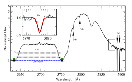
During the 2016 periastron passage of WR 140, we initiated a global spectroscopic campaign on the system similar to that described by Fahed et al. (2011). In total, our Pro-Am campaign collected 160 spectra over 323 days when the velocities were expected to be varying most rapidly. Our measurements are provided in the appendix of this paper in Table 6. The spectra all covered the C iii $\lambda 5696\text{\AA}$ emission-line (broad and narrow components emitted in the WR- and O star winds, respectively, and from the variable CW region) and the He i $\lambda 5876\text{\AA}$ line (with emission and P Cygni absorption components from the WR wind, a variable excess emission from the colliding-wind shock-cone, and an absorption component from the O star’s photosphere). In addition we downloaded archival ESPaDOnS spectra¹¹1http://polarbase.irap.omp.eu/ (Donati et al., 1997; Petit et al., 2014), and previously analyzed by de la Chevrotière et al. (2014). There were a total of 6 nights of data that were co-added to make a single spectrum for each night.

2.1.1 Radial Velocity Measurements

The properties of the spectra, and a journal of the observations, are shown in Table 1. With spectra from so many different sources, we had to ensure that the wavelength calibration was reliable among the various observatories. We therefore checked the alignment of the interstellar Na D absorption lines and Diffuse Interstellar Bands (DIBs) with locations indicated in Fig. 1 and wavelengths measured in the ESPaDOnS data. We then linearly shifted the data by no more than $1.3\text{\AA}$ to obtain a better wavelength solution. With four interstellar absorption lines, we were also able to ensure that the spectral dispersion was reliable for the data during this process. An example spectrum of the C iii $\lambda 5696\text{\AA}$ line is shown in Fig. 1.

Refer to caption — Figure 1: An example spectrum, collected on HJD 2457703.3, with annotations to illustrate the measurement process. On the left of is the flat-topped C iii line profile used for determining the radial velocity of the WR component of the system. The grey dashed lines correspond to the five normalized flux values use for bisection, with the extreme values marked to the left of the grey dashed lines. The small central peak near 5700 Å is the C iii component from the O star. The blue dot-dash line is the continuum, and the green regions on either side of the C iii profile contain the regions used for normalizing the feature. Two upward arrows indicate the locations of the DIBs used to check the wavelength calibration. The two downward arrows mark the interstellar Na i D-lines, also used to check the wavelength solution. The inset illustrates the normalized He i line from the O star, denoted by the box next to the Na i lines. The red curve is a Gaussian fit to the O star.

Table 1: List of contributed spectra, in order of number of spectra. The wavelength coverage and range of observation data for each primary observer are noted, as well as the approximate resolving power of their spectra. The average signal to noise ratio for each observer is also noted.

Observer	$N_{\rm spectra}$	$\lambda_{\rm start}$	$\lambda_{\rm end}$	HJD_first	HJD_end	Resolving	Average	Spectrograph	Aperature
		(Å)	(Å)	$-2450000.5$	$-2450000.5$	Power	S/N		(m)
Guarro	48	3979	7497	7666.89	7944.85	19,000	100	eSHEL	0.4
Thomas	26	5567	6048	7644.12	7918.07	15,000	50	LHIRES III	0.3
Leadbeater	17	5623	5968	7615.9	7788.73	15,000	173	LHIRES III	0.28
Ribeiro	16	5528	6099	7709.81	7762.76	16,000	70	LHIRES III	0.36
Garde	10	4185	7314	7624.91	7759.69	11,000	83	eSHEL	0.3
Berardi	12	5522	6002	7715.73	7778.71	15,000	180	LHIRES III	0.23
Campos	12	5463	6212	7675.86	7764.73	15,000	65	DADOS	0.36
Lester	9	5143	6276	7697.01	7769.94	17,000	118	LHIRES III	0.3
Ozuyar	6	4400	7397	7624.77	7730.68	12,000	85	eSHEL	0.4
ESPaDOnS	6	3691	10481	4645.59	8293.62	81,000	191	ESPaDOnS	3.58
Stober	1	4276	7111	7616.82	–	18,000	36	eSHEL	0.3

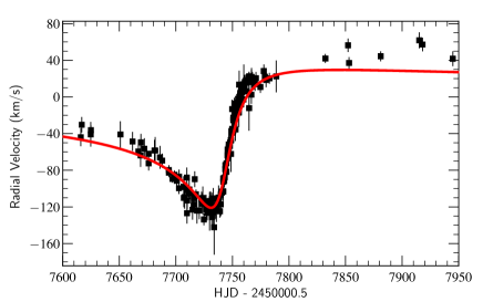
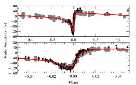
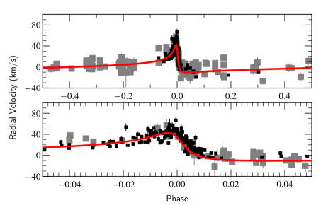
The velocities of the WR star, shown in the left panel of Fig. 2, were measured by bisecting the C iii $5696\text{\AA}$ emission plateau to find the centroid of the feature. We chose this line due to its relative isolation from other emission features. For example, the C iv $\lambda\lambda 5802,5812\text{\AA}$ doublet may have been a better choice, but is heavily blended with the He i $\lambda 5876\text{\AA}$ emission from the WR wind. The spectra were normalized with a linear function so that the low points on either side of the C iii feature had a flux of unity. The emission profile was bisected at normalized flux values, illustrated in Fig. 1, of: 1.1, 1.15, 1.2, 1.25, and 1.3. The velocity was then calculated for the average bisector. The displayed error bars take into account the standard deviation in the bisection velocity, the signal-to-noise in the continuum regions selected for the normalization, and the wavelength calibration. The errors were added in quadrature. It was found that the error is dominated by the standard deviation in the bisectors.

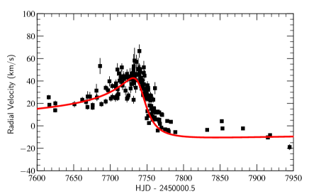
A few velocity measurements made just post HJD 2457800 do seem higher than expected for a Keplerian orbit, close examination of these spectra reveal that the colliding-wind excess is likely affecting the red shoulder of the C iii emission profile and skews the bisector toward higher redshift in our measurements. The variation in the location of the red shoulder corresponds to skew in the bisector of approximately 30 km s^-1, which is roughly the difference between the outliers and the model fit. We did not attempt to correct this, as the number of points affected was small, and this phase of the binary orbit has minimal changes in the radial velocity.

The O star velocities in the right panel of Fig. 2 were measured by fitting a Gaussian profile to the He i $\lambda 5875.621\text{\AA}$ helium absorption line, which never interferes with any P Cygni absorption from the WR star due to the high WR wind speed. When phase-folded, our O star velocities are consistent with velocities from a large range of absorption lines measured by Fahed et al. (2011). The displayed error bars for the O star velocities account for the uncertainty in the wavelength calibration, the standard deviation, and the uncertainty in the centroid of a Gaussian. We used the FWHM from our Gaussian profile in equation 15 of Garnir et al. (1987) to find the uncertainty in the centroid. The reported error is the quadrature sum of the errors. We found that the largest source of uncertainty in the centroid of the Gaussian fit was caused by the signal-to-noise in the continuum.

2.2 Interferometry with the CHARA Array

We have obtained four new epochs of CHARA Array interferometry to measure the precise astrometry of the component stars, following the work of Monnier et al. (2011). The first observation was obtained on 2011 June 17 with the CLIMB beam combiner (Ten Brummelaar et al., 2013). This observation consisted of five observations with the E1, W1, and W2 telescopes. Observations were calibrated with the same calibration stars as Monnier et al. (2011), with the observations of the calibration stars happening before and after each individual scan. These bracketed observations were made in the $K^{\prime}-$ band and reduced with a pipeline written by John D. Monnier, and were then combined into one measurement to improve the astrometric accuracy.

Another observation was obtained with the MIRC combiner (Monnier et al., 2012b) on UT 2011 September 16. The MIRC combiner uses all six telescopes of the CHARA Array, with eight spectral channels across the $H-$ band. The data were reduced using the MIRC data reduction pipeline (Monnier et al., 2007) using a coherent integration time of 17 ms. Monnier et al. (2012a) determined a correction factor for the absolute wavelength scale of MIRC data by analyzing the orbit of $\iota$ Peg. Based on that analysis, we multiplied the wavelengths in the calibrated data file by a factor of 1.004, appropriate for 6-telescope MIRC data collected between 2011-2017. Therefore, we applied this wavelength correction factor of 1.004 to the data based on the analysis by Monnier et al. (2012a). Two additional observations were obtained with the upgraded MIRC-X combiner (Kraus et al., 2018; Anugu et al., 2018, 2020) on UT 2018 October 26 and 2019 July 1. The observations were recorded in the PRISM50 mode which provides a spectral resolution of $R=50$ . The data were reduced using the MIRC-X data reduction pipeline, version 1.2.0²²2https://gitlab.chara.gsu.edu/lebouquj/mircx_pipeline.git. to produce calibrated visibilities and closure phases. During the reduction, we applied the bias correction included in the pipeline and set the number of coherent coadds to 5. A list of the calibrators and their angular diameters ( $\theta_{\rm UD}$ ) adopted from the JMMC catalog (Bourges et al., 2017) are listed in Table 2.

We analyzed the calibrated interferometric data using the same approach as Richardson et al. (2016). More specifically, we performed an adaptive grid search to find the best fit binary position and flux ratio ( $f_{\rm WR}/f_{\rm O}$ ) using software³³3This software is available at http://www.chara.gsu.edu/analysis-software/binary-grid-search. developed by Schaefer et al. (2016). During the binary fit, we fixed the uniform disk diameters of the components to sizes of 0.05 mas for the WR star and 0.07 mas for the O star as determined by Monnier et al. (2011). We added a contribution from excess, over-resolved flux to the binary fit that varied during each epoch. The uncertainties in the binary fit were derived by adding in quadrature errors computed from three sources: the formal covariance matrix from the binary fit, the variation in parameters when changing the coherent integration time used to reduce the data (17 ms and 75 ms for MIRC; 5 and 10 coherent coadds for MIRC-X), and the variation in parameters when changing the wavelength scale by the internal precision (0.25% for MIRC determined by Monnier et al. (2011); 0.5% for MIRC-X determined by Anugu et al. (2020)). In scaling the uncertainties in the position, we added the three values in quadrature for the major axis of the error ellipse ( $\sigma_{\rm major}$ ) and scaled the minor axis ( $\sigma_{\rm minor}$ ) to keep the axis ratio and position angle fixed according to the values derived from the covariance matrix. The results of the astrometric measurements are given in Table 3, with significant figures dependent on the individual measurements. In addition to the previously discussed parameters, we include the position angle of the error ellipse ( $\sigma_{\rm PA}$ ) in Table 3.

Table 2: Calibrator stars observed during the MIRC and MIRC-X observations at the CHARA Array.

Star	$\theta_{\rm UD}$ (mas)	Date Observed
HD 178538	0.2487 $\pm$ 0.0062	2019Jul01
HD 191703	0.2185 $\pm$ 0.0055	2019Jul01
HD 197176	0.2415 $\pm$ 0.0058	2019Jul01
HD 201614	0.3174 $\pm$ 0.0074	2019Jul01
HD 204050	0.4217 $\pm$ 0.0095	2018Oct26
HD 228852	0.5441 $\pm$ 0.0127	2018Oct26
HD 182564	0.3949 $\pm$ 0.0253	2011Sep16
HD 195556	0.2118 $\pm$ 0.0080	2011Sep16
HD 210839	0.4200 $\pm$ 0.0200	2011Sep16
HD 214734	0.3149 $\pm$ 0.0286	2011Sep16

Table 3: Interferometric measurements with the CHARA Array.

UT Date	HJD	Instrument	Bandpass	Separation	Position	$\sigma_{\rm major}$	$\sigma_{\rm minor}$	$\sigma_{\rm PA}$	$f_{\rm WR}/f_{\rm O}$	Excess Flux
	$-2450000.5$			(mas)	Angle (^∘)	(mas)	(mas)	(^∘)		(%)
2011Jun17	5729.411	CLIMB	$K^{\prime}$	13.02	153.00	0.22	0.06	162
2011Sep16	5820.270	MIRC	H	12.969	151.749	0.065	0.049	111.65	1.5665 $\pm$ 0.2257	5.94 $\pm$ 0.81
2018Oct26	8417.139	MIRC-X	H	11.932	155.969	0.060	0.043	141.12	1.1298 $\pm$ 0.0044	11.78 $\pm$ 0.12
2019Jul01	8665.351	MIRC-X	H	13.017	152.458	0.065	0.029	173.43	1.1006 $\pm$ 0.0063	1.31 $\pm$ 0.77

3 The Orbital Elements

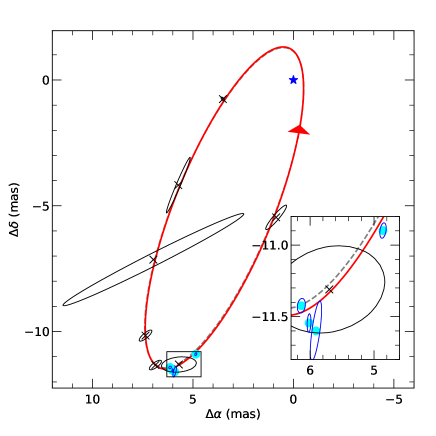
Orbital fits for massive stars with both high-quality spectroscopic and interferometric measurements have become more routine. For this work we simultaneously fit the spectroscopic and interferometric data using the method discussed in Schaefer et al. (2016), which was also used in Richardson et al. (2021). With the orbital solution from Monnier et al. (2011) as the starting point, the orbital models were simultaneously adjusted to fit radial velocities (from this work and Fahed et al. (2011)), and the interferometric measurements from this work, and from Monnier et al. (2011). The models are adjusted to minimize the $\chi^{2}$ statistic. We adopted a minimum 5 km s^-1 error on the radial velocities so that the radial velocity and astrometric data have similar weight in the final $\chi^{2}$ .

When we attempted to fit an orbit with measurements that had an error smaller than 5 km s^-1, we found that the solution would have a larger $\chi^{2}_{\rm red}$ than our adopted orbit due to their disproportionate weighting. We then increased the error in each measurement with a small error to 5 km s^-1 in order to fit our orbit. The visual orbit is shown in Fig. 3 and the spectroscopic orbit with all data included is shown in the two panels of Fig. 4.

Monnier et al. (2011) derived an orbital parallax for the system, which yielded a distance of 1.67 $\pm 0.03$ kpc. The Gaia Data Release 2 parallax (0.58 $~{}\pm~{}$ 0.03 mas) corresponds to a distance of 1.72 $\pm 0.09$ kpc. However, using the work of Bailer-Jones et al. (2018), we find that the Bayesian-inferred Gaia distance of 1.64 ${}^{+0.08}_{-0.07}$ kpc⁴⁴4We also note that Rate & Crowther (2020) derived a distance of 1.64 ${}^{+0.11}_{-0.09}$ kpc using Bayesian statistics and a prior tailored for WR stars for the astrometry from Gaia. is consistent with that of Monnier et al. (2011). The Bayesian-inferred distance is preferred as it corrects for the non-linearity of the transformation and uses an expected Galactic distribution of stars, being thoroughly tested against star clusters with known distances.

We also note that the EDR3 data from Gaia (Gaia Collaboration et al., 2020) suggest a parallax of 0.5378 $\pm$ 0.0237 mas, corresponding to a distance of 1.86 $\pm$ 0.08 kpc, which is well outside of the allowed distances from our orbit, the Gaia DR2 distance derived by either Bourges et al. (2017) or Rate & Crowther (2020). We speculate that this is because the EDR3 data will include data from near periastron when the photocenter seen by Gaia could shift quickly and thus interfere with excellent measurements usually given by Gaia. However, determining the actual source of the Gaia errors for WR 140’s parallax is beyond the scope of this paper.

Our derived orbital parameters, shown in lower half of Table 4, were calculated using our derived distance in the first column. The second column of the lower part of Table 4 shows our derived parameters calculated using the Gaia DR2 distance. The last column of Table 4 shows the results from Monnier et al. (2011) and Fahed et al. (2011) for easy reference. We note that the distance we derive is about 2 $\sigma$ away from the accepted Gaia DR2 distance of 1.67 kpc. While this level of potential disagreement may be concerning, we also note that the recent EDR3 data for Gaia was problematic, perhaps because the measurements happened across a periastron passage. We suspect that a proper treatment of the astrometry from Gaia with the orbital motion included may solve this discrepancy, but further analysis is beyond the scope of this paper.

We note that the masses of the O star are now lower when we allow our derived parameters to measure an orbital parallax. The mass of the WR star has a similar error as the analysis of Monnier et al. (2011), but is considerably lower. In fact, we are now in a prime position to compare the system to $\gamma^{2}$ Velorum (see the orbit presented by Lamberts et al., 2017), the only other WC star with a visual orbit. $\gamma^{2}$ Vel’s WC star has a spectral type of WC8, so is slightly cooler than the WR star in WR 140. Its mass is $\sim 9M_{\odot}$ , which is only slightly less than what we infer in our orbit.

Our derived masses are lower than those derived by Monnier et al. (2011) with the Fahed et al. (2011) spectroscopic orbit when using our derived orbit without the Gaia DR2 parallax, differing by at least 3 $\sigma$ . However, when we take into account the Gaia DR2 parallax, the masses are within 1 $\sigma$ of the values from the Monnier et al. (2011) analysis. The best way to solve any discrepancy in the future will be to improve the visual orbit and make use of any refinement of the Gaia parallax with future data releases.

O stars are very difficult to assign spectral types to in WR systems, due to extreme blending of the O and WR features in the optical spectrum. Fahed et al. (2011) found the O star to have a spectral type of O5.5fc, and the ‘fc’ portion of the spectral type means the star should have a luminosity class of I or III (e.g., Sota et al., 2011). While the Monnier et al. (2011) solution or our solution where we adopt the Gaia distance are broadly in agreement, our derived parameters suggest that the mass is lower. If we use the O star calibrations of Martins et al. (2005), then we see that the O star should have a later spectral type than given by Fahed et al. (2011), although the difficulties in assigning spectral types to the companion stars in WR binaries can certainly affect this measurement.

Table 4: Orbital elements calculated using all historical data plus the new data presented in this paper are in the column “This Work + Prior”. In the lower half of the table we provide the derived properties of the system. The work in this paper has two columns with values calculated from our determined distance using the visual orbit, and a second column where the parameters are calculated using the Gaia distance.

Derived Properties
Orbital Element	This Work +		Monnier 2011 +
	Prior		Fahed 2011
$P$ (days)	$2895.00\pm 0.29$		$2896.35\pm 0.20$
$T_{\scalebox{0.8}{$\scriptscriptstyle\rm 0$}}$ (MJD)	$60636.23\pm 0.53$		$46154.8\pm 0.8$
$e$	$0.8993\pm 0.0013$		$0.8964_{\scalebox{0.6}{$-0.0007$}}^{\scalebox{0.6}{$+0.0004$}}$
$\omega_{\scalebox{0.8}{$\scriptscriptstyle\rm WR$}}~{}(^{\circ})$	$227.44\pm 0.52$		$226.8\pm 0.4$
$K_{\scalebox{0.8}{$\scriptscriptstyle\rm O$}}$ (km s^-1)	$26.50\pm 0.48$		$30.9\pm 0.6$
$K_{\scalebox{0.8}{$\scriptscriptstyle\rm WR$}}$ (km s^-1)	$-75.25\pm 0.63$		$-75.5\pm 0.7$
$\gamma_{\scalebox{0.8}{$\scriptscriptstyle\rm O$}}$ (km s^-1)	$3.99\pm 0.37$		…
$\gamma_{\scalebox{0.8}{$\scriptscriptstyle\rm WR$}}$ (km s^-1)	$0.26\pm 0.32$		…
$i~{}(^{\circ})$	$119.07\pm 0.88$		$119.6\pm 0.5$
$\Omega~{}(^{\circ})$	$353.87\pm 0.67$		$353.6\pm 0.4$
$a$ (mas)	$8.922\pm 0.067$		$8.82\pm 0.05$
$\chi^{2}$	$1843.09$		…
$\chi^{2}_{\rm red}$	$2.01$		…
	Calculated Distance	Gaia Distance	Monnier 2011 +
	This Work	This Work	Fahed 2011
Distance (kpc)	$1.518\pm 0.021$	$1.64_{\scalebox{0.6}{$-0.07$}}^{\scalebox{0.6}{$+0.08$}}$	$1.67\pm 0.03$
$a$ (AU)	$13.55\pm 0.21$	$14.63\pm 0.049$	$14.7\pm 0.02$
$M_{\scalebox{0.8}{$\scriptscriptstyle\rm O$}}$ (M_⊙)	$29.27\pm 1.14$	$36.87\pm 4.34$	$35.9\pm 1.3$
$M_{\scalebox{0.8}{$\scriptscriptstyle\rm WR$}}$ (M_⊙)	$10.31\pm 0.45$	$12.99\pm 1.54$	$14.9\pm 0.5$
$q=\frac{M_{\scalebox{0.8}{$\scriptscriptstyle\rm WR$}}}{M_{\scalebox{0.8}{$\scriptscriptstyle\rm O$}}}$	$0.35\pm 0.01$	$0.35\pm 0.01$	$0.415\pm 0.002$

4 The Evolutionary History of WR 140

We have attempted to understand the evolutionary history and future of WR 140 by comparing its observational parameters to binary evolution models from the Binary Population And Spectral Synthesis (BPASS) code, v2.2.1 models, as described in detail in Eldridge et al. (2017) and Stanway & Eldridge (2018). Our fitting method is based on that in Eldridge (2009) and Eldridge & Relaño (2011). We use the $UBVJHK$ magnitudes taken from Ducati (2002) and Cutri et al. (2003). We note that the 2MASS magnitudes used here were measured in 1998, and thus were not contaminated by dust created in the 1993 IR maximum. To estimate the extinction, we take the $V$ -band magnitude from the BPASS model for each time-step and compare it to the observed magnitude. If the model $V$ -band flux is higher than observed, we use the difference to calculate the current value of $A_{V}$ . If the model flux is less than observed, we assume zero extinction. We then modify the rest of the model time-step magnitudes with this derived extinction before determining how well that model fits. Our derived value of $A_{V}$ is 2.4, which is in agreement with the current measurement of 2.46 (e.g., van der Hucht et al., 1988). We then also require that, for an acceptable fit, the model must have a primary star that is now hydrogen free, have carbon and oxygen mass fractions that are higher than the nitrogen mass fraction and that the masses of the components and their separation match the observed values that we determine here.

The one caveat in our fitting is that the BPASS models assume circular orbits; however, as found by Hurley et al. (2002), stars in orbits with the same semi-latus rectum, or same angular momentum, evolve in similar pathways independent of their eccentricity. A similar assumption was made in Eldridge (2009). While the orbit of WR 140 has not circularized, we note that in cases of binary interactions within an eccentric system, the tidally-enhanced mass transfer rate near periastron can cause a perturbation in the orbit that acts to increase the eccentricity with time rather than circularize the orbit, which is a possible explanation for the current observed orbit (e.g., Sepinsky et al., 2007a, b, 2009, 2010). We note that a more realistic model would require including the eccentricity. WR 140 is clearly a system where specific modelling of the interactions may lead to interesting findings on how eccentric binaries interact.

We considered a system to be matching if the masses were $M_{WR}/M_{\odot}=10.31\pm 1.99$ , and $M_{O}/M_{\odot}=29.27\pm 5.48$ . In selecting the period to match we use an assumption that systems with orbits that have the same semi-latus rectum are similar in their evolution. Thus taking account of the eccentricity we select models that have a separation of $log(a/R_{\odot})=2.746\pm 0.1$ .

Given this caveat, we find the current and initial parameters of the WR 140 system, as presented in Table 5. The values reported in Table 5 are the mean values of the considered models, with error bars being the standard deviation of those models averaged.

Table 5: Parameters from BPASS. The primary star evolved into the current WR star.

Initial Parameter	Value
$M_{\rm primary,i\rightarrow WR}$ ( $M_{\odot}$ )	$38.8\pm 6.0$
$M_{\rm O,i}$ ( $M_{\odot}$ )	$31.9\pm 1.3$
$\log(P_{\rm i}/d)$	$2.41\pm 0.30$
$Z$	$0.026\pm 0.011$
Present Parameter	Value
$A(V)$	$2.4\pm 0.2$
$\log({\rm Age}/yr)$	$6.70\pm 0.05$
$\log(L_{\rm primary\rightarrow WR}/L_{\odot})$	$5.31\pm 0.06$
$\log(L_{\rm O}/L_{\odot}))$	$5.48\pm 0.04$
$\log(T_{\rm primary,eff\rightarrow WR}/K)$	$5.05\pm 0.04$
$\log(T_{\rm O,eff}/K)$	$4.43\pm 0.04$

The matching binary systems tend to interact shortly after the end of the main sequence, thus the mass transfer events occur while the primary star still has a radiative envelope. This may explain why the orbit of WR 140 is still eccentric as deep convective envelopes are required for efficient circularization of a binary (Hurley et al., 2002). We also note that the mass transfer was highly non-conservative with much of the mass lost from the system. This is evident in that the orbit is significantly longer today than the initial orbit of the order of a year. The companion does accrete a few solar masses of material, so it is possible that the companion may have a significant rotational velocity. Additionally, the companion may be hotter than our models predict here due to the increase in stellar mass. However, we note that the average FWHM of the He i $\lambda 5876\text{\AA}$ line in velocity-space was 140 km s^-1, which if used as a proxy for the rotational velocity, $v\sin i$ , is fairly normal for young stellar clusters (e.g., Huang & Gies, 2006). If the O star rotates in the plane of the orbit, the rotational speed would be $\sim$ 160 km s^-1, slightly larger than typical O stars (e.g. Ramírez-Agudelo et al., 2013, 2015), but possibly less than predicted if significant accretion would have occurred (de Mink et al., 2013).

This could also be expected if the situation is as described by Shara et al. (2017) and Vanbeveren et al. (2018), where the O star’s spin-up of the companion could have been braked by the brief appearance of a strong global magnetic field generated in the process (Schneider et al., 2019). Indeed, while some WR+O binaries show some degree of spin-up, that degree is observed to be much less than expected initially after accretion.

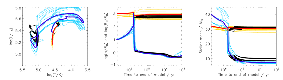
While this discussion has used the mean values from all the BPASS models considered, we have taken the most likely fitting binary and the closest model to this and show their evolution as the bold curves in Fig. 5. As we describe above the interactions are modest, because the primary loses a significant amount of mass through stellar winds before mass transfer begins in these models. The interaction is either a short common-envelope evolution which only shrinks the orbit slightly, or only a Roche lobe overflow with the orbit widening. In all cases the star would have become a Wolf-Rayet star without a binary interaction thus making the interactions modest since most mass loss was done via stellar winds.

The most confusing thing about WR 140 is the significantly low estimated age of only 5.0 Myrs ( $\log({\rm Age}/yr)=6.70$ ). There are relatively few other stars in the volume of space near WR 140 that would be members of a young cluster. It is therefore a good example of how sometimes clusters may form one very massive star rather than a number of lower-mass stars. The location of the stellar wh $\rm\bar{a}$ nau⁵⁵5The M $\rm\bar{a}$ ori word for extended family. is an open question in its history. It is difficult to make this system older, even if we assume that the Wolf-Rayet star could have been the result of evolution in a triple system and the result of a binary merger. Indeed, such a scenario would not explain how such a massive O star like the companion star could exist. Its presence sets a hard upper limit on the age of the system of approximately 5.0 Myrs.

5 Conclusions

We have presented an updated set of orbital elements for WR 140, using newly acquired spectroscopic and interferometric data combined with previously published measurements. We simultaneously fit all data to produce our orbital solution, and derived masses from our orbit of $M_{\rm WR}=10.31\pm 0.45M_{\odot}$ and $M_{\rm O}=29.27\pm 1.14M_{\odot}$ . We noted in our discussion that the O star mass seems a bit low given an earlier spectral classification, but that classification of O stars in WR systems is challenging. Future measurements of more WR binaries will be crucial to test stellar models. For WR 140, a detailed spectral model of the binary, as done for other WR binaries resolved with interferometry (e.g., Richardson et al., 2016) would allow for the derived parameters of the system to be used to constrain the models of WR stars and their winds.

We also discussed the possible evolutionary history of the system in comparison to the BPASS models. The results show that the majority of the envelope is lost by stellar winds with binary interactions only removing a modest amount of material. The measurements presented here should allow for more precise comparisons with the stellar evolutionary and wind models for massive (binary) stars in the future. Furthermore, these results will be used as a foundation for interpretation of multiple data sets that have been collected, including the X-ray variability (Corcoran et al., in prep) and wind collisions (Williams et al., 2021). While these orbital elements are well defined, future interferometric observations with MIRCX will allow for exquisite precision in new measurements, along with additional spectroscopic observational campaigns during periastron passages. MIRCX imaging at the times closest to periastron could pinpoint the location of the dust formation in the system, which could be observable in November 2024.

Acknowledgements

This work is based in part upon observations obtained with the Georgia State University Center for High Angular Resolution Astronomy Array at Mount Wilson Observatory. The CHARA Array is supported by the National Science Foundation under Grant No. AST-1636624 and AST-1715788. Institutional support has been provided from the GSU College of Arts and Sciences and the GSU Office of the Vice President for Research and Economic Development. Some of the time at the CHARA Array was granted through the NOAO community access program (NOAO PropID: 17A-0132 and 17B-0088; PI: Richardson). MIRC-X received funding from the European Research Council (ERC) under the European Union’s Horizon 2020 research and innovation programme (grant No. 639889). This work has made use of data from the European Space Agency (ESA) mission Gaia (https://www.cosmos.esa.int/gaia), processed by the Gaia Data Processing and Analysis Consortium (DPAC, https://www.cosmos.esa.int/web/gaia/dpac/consortium). Funding for the DPAC has been provided by national institutions, in particular the institutions participating in the Gaia Multilateral Agreement.

NDR acknowledges previous postdoctoral support by the University of Toledo and by the Helen Luedtke Brooks Endowed Professorship, along with NASA grant #78249. HS acknowledges support from the European Research Council (ERC) under the European Union’s DLV-772225-MULTIPLES Horizon 2020 and from the FWO-Odysseus program under project G0F8H6. JDM acknowledges support from AST-1210972, NSF 1506540 and NASANNX16AD43G. AFJM is grateful to NSERC (Canada) for financial aid. PMW is grateful to the Institute for Astronomy for continued hospitality and access to the facilities of the Royal Observatory. This research made use of Astropy,⁶⁶6http://www.astropy.org a community-developed core Python package for Astronomy (Astropy Collaboration et al., 2013; Price-Whelan et al., 2018).

Data Availability

All measurements used in this analysis are tabulated either in this paper or included in cited references.

References

Anugu et al. (2018) Anugu N., et al., 2018, in Proc. SPIE. p. 1070124 (arXiv:1807.03809), doi:10.1117/12.2313036
Anugu et al. (2020) Anugu N., et al., 2020, arXiv e-prints, p. arXiv:2007.12320
Astropy Collaboration et al. (2013) Astropy Collaboration et al., 2013, A&A, 558, A33
Bailer-Jones et al. (2018) Bailer-Jones C. A. L., Rybizki J., Fouesneau M., Mantelet G., Andrae R., 2018, AJ, 156, 58
Bourges et al. (2017) Bourges L., Mella G., Lafrasse S., Duvert G., Chelli A., Le Bouquin J. B., Delfosse X., Chesneau O., 2017, VizieR Online Data Catalog, p. II/346
Cutri et al. (2003) Cutri R. M., et al., 2003, VizieR Online Data Catalog, p. II/246
Donati et al. (1997) Donati J. F., Semel M., Carter B. D., Rees D. E., Collier Cameron A., 1997, MNRAS, 291, 658
Ducati (2002) Ducati J. R., 2002, VizieR Online Data Catalog, II/237,
Eldridge (2009) Eldridge J. J., 2009, MNRAS, 400, L20
Eldridge & Relaño (2011) Eldridge J. J., Relaño M., 2011, MNRAS, 411, 235
Eldridge et al. (2017) Eldridge J. J., Stanway E. R., Xiao L., McClelland L. A. S., Taylor G., Ng M., Greis S. M. L., Bray J. C., 2017, Publ. Astron. Soc. Australia, 34, e058
Fahed et al. (2011) Fahed R., et al., 2011, MNRAS, 418, 2
Gaia Collaboration et al. (2020) Gaia Collaboration et al., 2020, arXiv e-prints, p. arXiv:2012.02036
Garnir et al. (1987) Garnir H.-P., Baudinet-Robinet Y., Dumont P.-D., 1987, Nuclear Instruments and Methods in Physics Research B, 28, 146
Huang & Gies (2006) Huang W., Gies D. R., 2006, ApJ, 648, 580
Hurley et al. (2002) Hurley J. R., Tout C. A., Pols O. R., 2002, MNRAS, 329, 897
Kraus et al. (2018) Kraus S., et al., 2018, in Optical and Infrared Interferometry and Imaging VI. p. 1070123 (arXiv:1807.03794), doi:10.1117/12.2311706
Lamberts et al. (2017) Lamberts A., et al., 2017, MNRAS, 468, 2655
Lau et al. (2020) Lau R. M., Eldridge J. J., Hankins M. J., Lamberts A., Sakon I., Williams P. M., 2020, ApJ, 898, 74
Marchenko et al. (2003) Marchenko S. V., et al., 2003, ApJ, 596, 1295
Martins et al. (2005) Martins F., Schaerer D., Hillier D. J., 2005, A&A, 436, 1049
Monnier et al. (2007) Monnier J. D., et al., 2007, Science, 317, 342
Monnier et al. (2011) Monnier J. D., et al., 2011, ApJ, 742, L1
Monnier et al. (2012a) Monnier J. D., et al., 2012a, ApJ, 761, L3
Monnier et al. (2012b) Monnier J. D., Pedretti E., Thureau N., Che X., Zhao M., Baron F., ten Brummelaar T., 2012b, in Optical and Infrared Interferometry III. p. 84450Y, doi:10.1117/12.926433
North et al. (2007) North J. R., Tuthill P. G., Tango W. J., Davis J., 2007, MNRAS, 377, 415
Petit et al. (2014) Petit P., Louge T., Théado S., Paletou F., Manset N., Morin J., Marsden S. C., Jeffers S. V., 2014, PASP, 126, 469
Price-Whelan et al. (2018) Price-Whelan A. M., et al., 2018, AJ, 156, 123
Ramírez-Agudelo et al. (2013) Ramírez-Agudelo O. H., et al., 2013, A&A, 560, A29
Ramírez-Agudelo et al. (2015) Ramírez-Agudelo O. H., et al., 2015, A&A, 580, A92
Rate & Crowther (2020) Rate G., Crowther P. A., 2020, MNRAS, p. 34
Richardson et al. (2016) Richardson N. D., et al., 2016, MNRAS, 461, 4115
Richardson et al. (2017) Richardson N. D., et al., 2017, MNRAS, 471, 2715
Schaefer et al. (2016) Schaefer G. H., et al., 2016, AJ, 152, 213
Schneider et al. (2019) Schneider F. R. N., Ohlmann S. T., Podsiadlowski P., Röpke F. K., Balbus S. A., Pakmor R., Springel V., 2019, Nature, 574, 211
Sepinsky et al. (2007a) Sepinsky J. F., Willems B., Kalogera V., 2007a, ApJ, 660, 1624
Sepinsky et al. (2007b) Sepinsky J. F., Willems B., Kalogera V., Rasio F. A., 2007b, ApJ, 667, 1170
Sepinsky et al. (2009) Sepinsky J. F., Willems B., Kalogera V., Rasio F. A., 2009, ApJ, 702, 1387
Sepinsky et al. (2010) Sepinsky J. F., Willems B., Kalogera V., Rasio F. A., 2010, ApJ, 724, 546
Shara et al. (2017) Shara M. M., Crawford S. M., Vanbeveren D., Moffat A. F. J., Zurek D., Crause L., 2017, MNRAS, 464, 2066
Sota et al. (2011) Sota A., Maíz Apellániz J., Walborn N. R., Alfaro E. J., Barbá R. H., Morrell N. I., Gamen R. C., Arias J. I., 2011, ApJS, 193, 24
Stanway & Eldridge (2018) Stanway E. R., Eldridge J. J., 2018, MNRAS, 479, 75
Sugawara et al. (2015) Sugawara Y., et al., 2015, PASJ, 67, 121
Ten Brummelaar et al. (2013) Ten Brummelaar T. A., et al., 2013, Journal of Astronomical Instrumentation, 2, 1340004
Vanbeveren et al. (2018) Vanbeveren D., Mennekens N., Shara M. M., Moffat A. F. J., 2018, A&A, 615, A65
Williams et al. (1978) Williams P. M., Beattie D. H., Lee T. J., Stewart J. M., Antonopoulou E., 1978, MNRAS, 185, 467
Williams et al. (1990) Williams P. M., van der Hucht K. A., Pollock A. M. T., Florkowski D. R., van der Woerd H., Wamsteker W. M., 1990, MNRAS, 243, 662
Williams et al. (2009) Williams P. M., et al., 2009, MNRAS, 395, 1749
Williams et al. (2021) Williams P. M., et al., 2021, MNRAS, 503, 643
de Mink et al. (2013) de Mink S. E., Langer N., Izzard R. G., Sana H., de Koter A., 2013, ApJ, 764, 166
de la Chevrotière et al. (2014) de la Chevrotière A., St-Louis N., Moffat A. F. J., MiMeS Collaboration 2014, ApJ, 781, 73
van der Hucht et al. (1988) van der Hucht K. A., Hidayat B., Admiranto A. G., Supelli K. R., Doom C., 1988, A&A, 199, 217

Appendix A Radial Velocity Measurements

Table 6: Measured radial velocities for the new spectra presented in this paper.

HJD $-2450000.5$	WR Velocity	O Velocity	Source
	(km/s)	(km/s)
4645.59101	$-42.8$ $\pm$ 5.5	$17.2$ $\pm$ 1.7	ESPaDOnS
4703.46011	$-48.3$ $\pm$ 3.2	$10.7$ $\pm$ 1.1	ESPaDOnS
4755.28504	$-58.2$ $\pm$ 5.9	$14.4$ $\pm$ 1.3	ESPaDOnS
5722.38773	$27.6$ $\pm$ 2.9	$-8.9$ $\pm$ 1.0	ESPaDOnS
7615.9085	$-44.0$ $\pm$ 9.8	$25.5$ $\pm$ 2.0	Leadbeater
7616.82776	$-30.3$ $\pm$ 8.5	$18.8$ $\pm$ 1.2	Stober
7624.76623	$-40.8$ $\pm$ 13.5	$13.8$ $\pm$ 1.8	Ozuyar
7624.91809	$-36.2$ $\pm$ 5.1	$20$ $\pm$ 2.4	Garde
7651.01573	$-40.9$ $\pm$ 14.4	$19.3$ $\pm$ 2.7	Thomas
7661.76968	$-48.6$ $\pm$ 10.4	$23.2$ $\pm$ 2.5	Ozuyar
7666.89338	$-59.5$ $\pm$ 7.3	$21.4$ $\pm$ 2.7	Guarro
7668.83826	$-63.8$ $\pm$ 12.4	$16.8$ $\pm$ 2.2	Guarro
7669.09369	$-49.6$ $\pm$ 9.4	$26.1$ $\pm$ 4.7	Thomas
7672.14171	$-56.6$ $\pm$ 11.4	$26.1$ $\pm$ 4.1	Thomas
7675.86058	$-62.0$ $\pm$ 2.4	$16.2$ $\pm$ 2.0	Campos
7675.89578	$-72.4$ $\pm$ 7.8	$18.5$ $\pm$ 2.2	Guarro
7681.06131	$-58.5$ $\pm$ 11.6	$31.4$ $\pm$ 6.0	Thomas
7681.7328	$-58.4$ $\pm$ 14.6	$25.2$ $\pm$ 3.1	Ozuyar
7685.99396	$-66.0$ $\pm$ 12.5	$53.3$ $\pm$ 7.1	Thomas
7687.88062	$-69.5$ $\pm$ 7.8	$19.4$ $\pm$ 2.4	Guarro
7693.78032	$-82.7$ $\pm$ 4.9	$33.9$ $\pm$ 2.6	Leadbeater
7693.78366	$-79.7$ $\pm$ 5.2	$21.7$ $\pm$ 2.5	Guarro
7697.01575	$-89.4$ $\pm$ 4.1	$31.7$ $\pm$ 3.1	Lester
7698.83037	$-85.0$ $\pm$ 4.7	$39.7$ $\pm$ 4.5	Guarro
7700.83225	$-91.5$ $\pm$ 9.0	$24.4$ $\pm$ 2.7	Guarro
7702.75581	$-99.5$ $\pm$ 6.4	$35.5$ $\pm$ 2.5	Leadbeater
7702.87022	$-87.1$ $\pm$ 7.8	$25.7$ $\pm$ 2.9	Guarro
7706.85286	$-97.9$ $\pm$ 11.3	$25.4$ $\pm$ 2.6	Guarro
7707.0665	$-110.1$ $\pm$ 10.1	$24.7$ $\pm$ 3.3	Thomas
7707.74176	$-109.3$ $\pm$ 12.6	$37.8$ $\pm$ 3.4	Leadbeater
7707.77422	$-98.4$ $\pm$ 5.4	$34.8$ $\pm$ 3.6	Guarro
7709.69196	$-88.0$ $\pm$ 11	$50.2$ $\pm$ 5.6	Ozuyar
7709.81017	$-126.8$ $\pm$ 11.3	$27.2$ $\pm$ 4.7	Ribeiro
7709.81296	$-101.8$ $\pm$ 8.2	$24.8$ $\pm$ 2.6	Guarro
7710.04092	$-113.1$ $\pm$ 9.5	$32.7$ $\pm$ 6.1	Thomas
7711.07536	$-104.4$ $\pm$ 5.0	$28.3$ $\pm$ 5.0	Thomas
7711.84949	$-101.0$ $\pm$ 12.6	$46.7$ $\pm$ 4.7	Leadbeater
7712.70276	$-105.0$ $\pm$ 6.7	$40.2$ $\pm$ 3.1	Leadbeater
7714.75764	$-123.0$ $\pm$ 10.8	$43.5$ $\pm$ 6.2	Ribeiro
7715.71599	$-117.4$ $\pm$ 5.8	$52.1$ $\pm$ 3.5	Leadbeater
7715.73729	$-110.7$ $\pm$ 5.4	$39.2$ $\pm$ 3.0	Beradi
7716.69472	$-89.7$ $\pm$ 8.6	$35.9$ $\pm$ 4.0	Ozuyar
7717.79801	$-106.2$ $\pm$ 5.3	$44.2$ $\pm$ 4.4	Guarro
7718.71246	$-124.1$ $\pm$ 14.1	$41.8$ $\pm$ 4.9	Garde
7720.77745	$-123.9$ $\pm$ 9.6	$31.4$ $\pm$ 4.1	Ribeiro
7722.74233	$-110.8$ $\pm$ 7.5	$44.4$ $\pm$ 4.5	Guarro
7722.77181	$-116.7$ $\pm$ 6.8	$46.2$ $\pm$ 4.1	Beradi
7722.80655	$-111.7$ $\pm$ 6.7	$24.2$ $\pm$ 3.3	Campos
7723.74669	$-113.0$ $\pm$ 15.3	$25.4$ $\pm$ 2.9	Campos
7723.75284	$-110.2$ $\pm$ 5.6	$43.1$ $\pm$ 4.3	Guarro
7724.74938	$-116.3$ $\pm$ 3.8	$44$ $\pm$ 4.4	Guarro
7724.75337	$-133.7$ $\pm$ 6.4	$27.1$ $\pm$ 3.1	Campos
7726.68947	$-113.7$ $\pm$ 6.8	$41.6$ $\pm$ 4.4	Garde
7727.06099	$-122.6$ $\pm$ 10.6	$43.6$ $\pm$ 7.9	Thomas
7727.76572	$-126.4$ $\pm$ 8.2	$33.4$ $\pm$ 4.1	Ribeiro
7728.75588	$-121.2$ $\pm$ 7.1	$37.2$ $\pm$ 4.3	Ribeiro
7729.72349	$-118.0$ $\pm$ 3.2	$46.4$ $\pm$ 4.9	Guarro
7729.79283	$-124.7$ $\pm$ 21.1	$44.8$ $\pm$ 6.3	Campos
7730.68289	$-113.7$ $\pm$ 10.7	$43.6$ $\pm$ 5.3	Ozuyar

Table 7: continued

Measured radial velocities for the new spectra presented in this paper. HJD $-2450000.5$ WR Velocity O Velocity Source (km/s) (km/s) 7730.73046 $-123.2$ $\pm$ 8.2 $47$ $\pm$ 5 Guarro 7731.69913 $-119.2$ $\pm$ 6.4 $50.2$ $\pm$ 3.8 Beradi 7731.74248 $-119.5$ $\pm$ 7.1 $38$ $\pm$ 3.8 Guarro 7731.7559 $-131.2$ $\pm$ 9.1 $41.2$ $\pm$ 5 Ribeiro 7731.76974 $-111.5$ $\pm$ 7.1 $23.2$ $\pm$ 3.4 Campos 7732.00337 $-122.5$ $\pm$ 9.7 $53$ $\pm$ 10.9 Thomas 7732.6973 $-123.5$ $\pm$ 9.8 $44.8$ $\pm$ 5.8 Garde 7732.89655 $-125.9$ $\pm$ 14.5 $46.1$ $\pm$ 4.1 Leadbeater 7733.04298 $-110.7$ $\pm$ 11.2 $58.2$ $\pm$ 11.3 Thomas 7733.78171 $-142.2$ $\pm$ 29.9 $46.3$ $\pm$ 8.8 Campos 7734.74934 $-119.8$ $\pm$ 6.2 $40.6$ $\pm$ 3.9 Guarro 7734.75611 $-124.0$ $\pm$ 9.5 $34$ $\pm$ 4.6 Ribeiro 7735.69391 $-123.5$ $\pm$ 8.8 $45.4$ $\pm$ 4.8 Garde 7735.73915 $-122.6$ $\pm$ 13.8 $57$ $\pm$ 6.3 Guarro 7737.75114 $-109.7$ $\pm$ 13.2 $50.7$ $\pm$ 5.4 Guarro 7737.99405 $-112.2$ $\pm$ 6.5 $50.4$ $\pm$ 10.1 Thomas 7738.92489 $-124.7$ $\pm$ 6.9 $46.2$ $\pm$ 7.7 Thomas 7739.69769 $-117.2$ $\pm$ 13 $66.6$ $\pm$ 5.9 Leadbeater 7739.72805 $-106.5$ $\pm$ 7.9 $50.6$ $\pm$ 5.1 Guarro 7740.70156 $-104.4$ $\pm$ 7.9 $50.3$ $\pm$ 4.1 Beradi 7740.72612 $-103.3$ $\pm$ 4.6 $48.2$ $\pm$ 4.8 Guarro 7741.75243 $-102.9$ $\pm$ 10.5 $42.9$ $\pm$ 6.5 Ribeiro 7741.93606 $-88.6$ $\pm$ 4.7 $39$ $\pm$ 4 Lester 7741.95381 $-103.3$ $\pm$ 6.9 $41.2$ $\pm$ 8 Thomas 7741.96782 $-89.3$ $\pm$ 8.3 $35.4$ $\pm$ 3.6 Lester 7741.99769 $-92.7$ $\pm$ 9.4 $40.3$ $\pm$ 4.1 Lester 7742.75752 $-91.5$ $\pm$ 7.2 $33.3$ $\pm$ 4.1 Ribeiro 7743.22505 $-87.8$ $\pm$ 7.8 $40.8$ $\pm$ 2.8 ESPaDOnS 7743.70079 $-78.9$ $\pm$ 9.4 $39.5$ $\pm$ 3 Beradi 7743.75725 $-74.3$ $\pm$ 12.5 $35.3$ $\pm$ 3.9 Guarro 7744.75494 $-81.6$ $\pm$ 6.6 $28.7$ $\pm$ 3.5 Ribeiro 7744.76281 $-72.4$ $\pm$ 6.6 $27.4$ $\pm$ 3 Guarro 7745.70176 $-63.4$ $\pm$ 8.4 $47.2$ $\pm$ 3.9 Beradi 7745.72762 $-57.4$ $\pm$ 10.9 $52.1$ $\pm$ 5.8 Guarro 7745.74729 $-64.0$ $\pm$ 8.7 $37.2$ $\pm$ 4.3 Campos 7746.74793 $-55.1$ $\pm$ 5.5 $44.7$ $\pm$ 4.9 Guarro 7746.76355 $-51.8$ $\pm$ 17.7 $33$ $\pm$ 4.9 Campos 7747.75535 $-53.4$ $\pm$ 16.9 $30.9$ $\pm$ 4.4 Garde 7748.70943 $-46.8$ $\pm$ 11.4 $26.2$ $\pm$ 2.4 Beradi 7748.72376 $-47.3$ $\pm$ 13.8 $24.2$ $\pm$ 2.6 Guarro 7748.75753 $-62.3$ $\pm$ 19.7 $31.6$ $\pm$ 4.6 Ribeiro 7749.70118 $-39.0$ $\pm$ 13.9 $27.5$ $\pm$ 2.3 Beradi 7749.72075 $-34.9$ $\pm$ 12.7 $28.3$ $\pm$ 2.9 Guarro 7749.75724 $-13.2$ $\pm$ 10.1 $6.8$ $\pm$ 1 Ribeiro 7750.69524 $-37.3$ $\pm$ 12.6 $35.8$ $\pm$ 2.8 Leadbeater 7750.71981 $-22.7$ $\pm$ 11.4 $36.1$ $\pm$ 3.7 Guarro 7750.75891 $-25.3$ $\pm$ 6.1 $13.1$ $\pm$ 1.5 Ribeiro 7751.70041 $-24.2$ $\pm$ 7.8 $32.1$ $\pm$ 3.9 Garde 7751.72145 $-19.2$ $\pm$ 11.5 $33.8$ $\pm$ 3.4 Guarro 7751.75795 $-7.1$ $\pm$ 6.2 $8.9$ $\pm$ 1.2 Ribeiro 7751.75888 $-28.9$ $\pm$ 12.3 $26.3$ $\pm$ 3.6 Campos 7752.69799 $-13.2$ $\pm$ 7.7 $23.6$ $\pm$ 2.9 Garde 7752.7211 $-7.7$ $\pm$ 8.9 $25.3$ $\pm$ 2.6 Guarro 7752.73721 $-35.4$ $\pm$ 12.7 $2.5$ $\pm$ 0.8 Campos 7753.72269 $-8.1$ $\pm$ 9.2 $18.2$ $\pm$ 1.8 Guarro 7754.69082 $-6.4$ $\pm$ 13 $27.1$ $\pm$ 3.2 Garde 7754.7034 $-9.8$ $\pm$ 10.2 $22.5$ $\pm$ 1.6 Beradi 7754.94876 $-7.3$ $\pm$ 15.5 $26.1$ $\pm$ 3.6 Thomas 7755.70308 $-16.8$ $\pm$ 15.9 $26.6$ $\pm$ 2.3 Leadbeater

Table 8: continued

Measured radial velocities for the new spectra presented in this paper. HJD $-2450000.5$ WR Velocity O Velocity Source (km/s) (km/s) 7755.94031 $-2.2$ $\pm$ 11.7 $15.8$ $\pm$ 1.6 Lester 7755.9461 $13.4$ $\pm$ 15.2 $17.7$ $\pm$ 2.3 Thomas 7755.963 $0$ $\pm$ 10.2 $10.5$ $\pm$ 1.2 Lester 7756.74935 $1.3$ $\pm$ 9.9 $14.8$ $\pm$ 1.8 Guarro 7757.70237 $3.8$ $\pm$ 11.2 $8.3$ $\pm$ 1 Beradi 7757.70469 $-8.3$ $\pm$ 12.2 $13.3$ $\pm$ 1.2 Leadbeater 7757.72899 $8.5$ $\pm$ 5.1 $5.5$ $\pm$ 0.9 Guarro 7758.72732 $5.1$ $\pm$ 10.1 $23.3$ $\pm$ 2.5 Guarro 7759.69877 $10.1$ $\pm$ 11.2 $15.7$ $\pm$ 1.8 Garde 7759.72275 $9.2$ $\pm$ 8.3 $12.3$ $\pm$ 1.4 Guarro 7759.76482 $-2.7$ $\pm$ 2.9 $15$ $\pm$ 2 Ribeiro 7759.97778 $14$ $\pm$ 21.4 $6.3$ $\pm$ 1.4 Thomas 7760.73924 $11.9$ $\pm$ 3.4 $7.5$ $\pm$ 1 Guarro 7760.95617 $16.3$ $\pm$ 7.7 $33.6$ $\pm$ 5.3 Thomas 7761.95875 $15.5$ $\pm$ 9.1 $12$ $\pm$ 1.3 Lester 7762.74853 $18.3$ $\pm$ 6.3 $11.8$ $\pm$ 1.4 Guarro 7762.76955 $6.3$ $\pm$ 5.1 $5.8$ $\pm$ 1 Ribeiro 7764.7039 $16.1$ $\pm$ 11.1 $5.8$ $\pm$ 0.8 Beradi 7764.72541 $22.5$ $\pm$ 4.9 $12.7$ $\pm$ 1.5 Guarro 7764.73166 $-12.1$ $\pm$ 24.7 $-4.1$ $\pm$ 1 Campos 7766.72684 $20.7$ $\pm$ 9.4 $5$ $\pm$ 0.8 Guarro 7766.74306 $2.5$ $\pm$ 10 $11.9$ $\pm$ 1.4 Leadbeater 7766.94453 $19.7$ $\pm$ 11.9 $3.9$ $\pm$ 0.7 Lester 7766.96052 $21.8$ $\pm$ 7.3 $5.5$ $\pm$ 1 Thomas 7767.73057 $18.5$ $\pm$ 8.5 $1.9$ $\pm$ 0.7 Guarro 7769.73312 $15.2$ $\pm$ 7.3 $-1.6$ $\pm$ 0.7 Guarro 7769.94296 $13.8$ $\pm$ 7.3 $10.4$ $\pm$ 1.2 Lester 7770.75387 $20.4$ $\pm$ 6.8 $9.7$ $\pm$ 1.3 Guarro 7774.71494 $10.8$ $\pm$ 6.4 $-3.2$ $\pm$ 0.8 Leadbeater 7777.73525 $28.3$ $\pm$ 7.1 $4.4$ $\pm$ 0.8 Guarro 7778.71117 $22.1$ $\pm$ 6.1 $-3.7$ $\pm$ 0.7 Beradi 7779.72978 $18.5$ $\pm$ 8 $-5.0$ $\pm$ 0.8 Leadbeater 7782.7386 $20.3$ $\pm$ 5.9 $3.6$ $\pm$ 0.8 Leadbeater 7788.73838 $22.4$ $\pm$ 17.4 $-5.6$ $\pm$ 0.9 Leadbeater 7832.19508 $42$ $\pm$ 4.9 $-3.6$ $\pm$ 0.8 Guarro 7852.19978 $56.3$ $\pm$ 7.3 $4.1$ $\pm$ 0.9 Thomas 7853.13919 $37.1$ $\pm$ 6.3 $-2.3$ $\pm$ 0.7 Guarro 7881.13262 $44.4$ $\pm$ 5.4 $-2.3$ $\pm$ 0.7 Guarro 7915.14428 $61.8$ $\pm$ 8.7 $-10.3$ $\pm$ 1.4 Thomas 7918.07741 $57.2$ $\pm$ 7.4 $-8.3$ $\pm$ 1.2 Thomas 7944.85441 $41.7$ $\pm$ 8.1 $-18.9$ $\pm$ 2.5 Guarro 8293.62071 $19.3$ $\pm$ 8.1 $-15.3$ $\pm$ 1.2 ESPaDOnS