The Number of Transits Per Epoch
for Transiting Misaligned Circumbinary Planets
1Dept. of Astronomy, Columbia University, New York, NY 10027, USA
Abstract
The growing catalog of circumbinary planets strengthens the notion that planets form in a diverse range of conditions across the cosmos. Transiting circumbinary planets yield especially important insights and many examples are now known, in broadly coplanar obits with respect to their binary. Studies of circumbinary disks suggest misaligned transiting examples could also plausibly exist, but their existence would exacerbate the already challenging feat of automatic detection. In this work, we synthesize populations of such planets and consider the number of transits per epoch they produce, forming integer sequences. For isotropic distributions, such sequences will appear foreign to conventional expectation, rarely (%) producing the signature double-transits we’ve come to expect for circumbinaries, instead producing sparse sequences dominated by zero-transit epochs (%). Despite their strangeness, we demonstrate that these sequences will be non-random and that the two preceding epochs predict the next to high accuracy. Additionally, we show that even when clustering the transits into grouped epochs, they often appear unphysical if erroneously assuming a single star, due to the missing epochs. Crucially, missing epochs mean highly isotropic populations can trick the observer into assigning the wrong period in up to a quarter of cases, adding further confusion. Finally, we show that the transit sequences encode the inclination distribution and demonstrate a simple inference method that successfully matches the injected truth. Our work highlights how the simple act of flagging transits can be used to provide an initial, vetting-level analysis of misaligned transiting circumbinary planets.
keywords:
binaries: general – techniques: photometric – planet and satellites: detection1 Introduction
Binary star systems represent a manifestly frequent outcome of star formation (Pringle, 1989; Chapman et al., 1992; Tohline, 2002). Indeed, the majority of Solar type stars reside within binary or higher multiplicity systems (Karttunen et al., 1994; Raghavan et al., 2010) - defying preconceptions one might foster through arguments of mediocrity. This naturally raises questions about the prevalance of planets around such binaries, which may exist in so-called “S-type” (orbiting just one of the stars) or “P-type” (orbiting both) configurations (Dvorak, 1986). For binary stars separated by less than 50 AU, observations reveal a clear dearth of S-type planets (Kraus et al., 2016), although counter-examples such as Cephei Ab (Hatzes et al., 2003) and KOI-1257 Ab (Santerne et al., 2014) demonstrate that a population does indeed exist. Further, simulation work concurs that planet formation is expected to be generally suppressed for S-type orbits in close binaries (e.g. see Thebault & Haghighipour 2015 and references therein).
For P-type orbits, so-called circumbinary planets (or even “Tatooines”), the situation is quite different. Many circumbinary planets have been discovered via transits (Welsh et al., 2012b), characterised by their elaborate light curves featuring one or more dips per epoch, of varying depths, durations and timings (e.g. Doyle et al. 2011). Unlike S-type planets, occurrence rate estimates suggest that giant circumbinary planets ( ) orbiting within 300 days are just as common as single stars (Armstrong et al., 2014).
Two key observations from this population are highlighted. The first is that there is a conspicuous absence of planets around the tightest main sequence binaries, consistent with such binaries forming through a phase of destructive inward migration (Muñoz & Lai, 2015; Hamers et al., 2016; Xu & Lai, 2016). The second is that there is a dearth of short-period circumbinary planets, and a pile-up close to a critical period of dynamical instability (Welsh et al., 2012a). This boundary of instabiltiy was characterised with a simple semi-empirical formula in Holman & Wiegert (1998) but was later extended to account for resonance instabilities independently by Lam & Kipping (2018) and Quarles et al. (2018).
Despite these advances, our view of these systems may not be complete. In particular, there may be a missing population of circumbinary planets - those which are misaligned to their binary. Armstrong et al. (2014) note that their occurrence rate estimate should be treated as a lower-limit, since a misaligned population could not be ruled out. Martin & Triaud (2014) show that misaligned systems would lead to even stranger transit sequences, featuring epochs with missing transits that would be challenging to identify in the first place. At first glance, such transit sequences may ostensibly appear “random”, making automated discovery difficult. The “Random Transiter” (HD 139139) exemplifies111We note that here both P- and S-type planetary transits were indeed hypothesised by Rappaport et al. (2019), but ultimately found to inadequately explain their data. the challenge of working with irregular sequences like this (Rappaport et al., 2019). So difficult these sequences are that Martin (2018) comments that “transit discovery methods that are sensitive to highly misaligned planets are yet to be demonstrated”.
A population of inclined circumbinary planets would thus clearly prove a challenge to existing detection algorithms, but would also provide unique insights into these enigmatic systems. Imaging of young binary systems provides some guidance as to whether such a population might exist, by measuring the alignment between the protoplanetary disks (from which planets form) and the binary (measured spectrosopically/astrometrically). Czekala et al. (2019) constrain that 68% of circumbinary disks are aligned to within for binaries with periods shorter than 20 days, but beyond 30 days one finds a diverse range up to polar orbiting disks. Whilst our knowledge here is clearly incomplete, a population of inclined circumbinary planets is consistent with current observations.
Conventional transit search algorithms, such as the “Box Least Squares” (BLS) algorithm (Kovács et al., 2002), utterly fail for even aligned circumbinary planets. This is because they assume strict periodicity between transits, but the binary’s constantly changing position imparts large timing and duration changes. As a result, early Kepler detections were largely conducted by eye (Doyle et al., 2011; Welsh et al., 2012b). A modification of BLS, designed for planets orbiting single stars plus some timing perturbation, dubbed QATS (“Quasiperiodic Automated Transit Search”) offers a possible improvement, but still does not account for the variable durations or the possibility of two dips (Carter & Agol, 2013). Efforts to modify BLS specifically for circumbinary planets have previously been made, such as the method of Klagyivik et al. (2017) that allows both the depth and duration of the transits to freely vary. However, the use of a large timing window to scan over introduces a higher false positive rate. Windemuth et al. (2019) offer the most advanced model to date, dubbed QATS-EB, using a simplified, semi-analytic model for the binary motion. However, even here, the method is forced to make numerous simplifying assumptions which may limit the sensitivity to extreme systems.
Clearly, as noted by Windemuth et al. (2019), one could relax these limitations by conducting searches using a fully photodynamical model, but the high dimensionality of the problem makes such a search impractical. Simplified models are clearly needed to enable the rapid analysis of ever growing databases of light curves, and in that context we might begin by simply asking - what do the light curves of transiting misaligned circumbinary planets look like?
Perhaps the most basic observable one might consider in this effort is the number of transits that occur each epoch. For a single star this always equals unity. But, as noted earlier, aligned circumbinary planets generally cause two transits Martin & Triaud (2014). During a syzygy event, one transit would be expected and for a very short-period binary and long-period planet one could observe more than two transits. Misaligned systems add even more complexity though by permitting zero-transit epochs. This makes automated detection immediately more challenging since now the transit sequence becomes sparse, and creates “broken” sequences where even the clustered transits don’t appear to follow a linear ephemeris. Indeed, such sequences might appear ostensibly random and be rejected by conventional algorithms demanding some pattern in the data.
In this work, then, we tackle the issue as to how many transits per epoch one expects for transiting misaligned circumbinary planets. If the transits are individually of sufficient high signal-to-noise, it should be possible to construct a catalog of the transit times which could then be clustered into groups representative of epochs. Individual transits are demonstrably discoverable either by citizen scientists (e.g. Eisner et al. (2021)) or an automated routine sensitive to single events of potentially highly peculiar shape (such as the “weird detector” algorithm; Wheeler & Kipping 2019). This work seeks to build some intuition and understanding of how these sequences would appear in our data, and how they could be ultimately used to make progress in the detection and interpretation of a misaligned circumbinary population.
In Section 2, we demonstrate that non-isotropic circumbinary planet populations are non-random by developing a memory slot prediction algorithm and showing that it outperforms random predictions. In Section 3, we establish a relationship between the observed transits per epoch counts and the inclination distribution of a circumbinary planet population. Based on this relationship, we develop a Bayesian framework to infer the inclination distribution of a circumbinary planet population. In Section 4, we conclude by discussing the challenges and opportunities that misaligned circumbinary systems pose to future works.
2 Randomness of Circumbinary Planet Transit Sequences
2.1 Random Worlds
As discussed in Section 1, this paper primarily concerns - how many transits per epoch does one expect for transiting misaligned circumbinary planets? The number of transits per epoch is perhaps the simplest observable one might reasonably define for such systems, yet we lack a good understanding of its behaviour. Figure 1 graphically illustrates how a circumbinary planet can cause zero, one or two transits. Indeed, more than two transits is also possible if the binary motion is sufficiently fast to “catch up” with the planet again during a given epoch. This case is challenging to graphically illustrate, and thus is not shown explicitly in Figure 1, but it is fully considered in what follows.

In light of this, a series of transit epochs will manifest a potentially variable number of transits each time. For example, the first epoch might yield two transits, the next epoch yields zero, the third epoch just a single dip, and so on. Such a series could be compactly represented using the digits “201…”. From the observer’s perspective, the true nature of the system is of course not immediately obvious; they are simply faced with a particular sequence and need to try to interpret the underlying cause.
The “Random Transiter” (Rappaport et al., 2019) again provides an analogous example of this situation. Rather than seeing a sequence of clustered events of varying counts (as is the case for circumbinary planets), Rappaport et al. (2019) instead report non-clustered transits scattered across the time series. Despite this difference, the problem is ostensibly similar to ours in that the lack of any clear pattern in the transits was confounding and unusual. A basic conclusion of their work is that the sequence was consistent with being produced from a random number generator. If indeed the transit times are truly stochastic, then it would be impossible to ever predict when the next transit would occur based on the previous data. This determination of randomness, if verified with future data, is important because one might hypothesise that complex, chaotic systems (e.g. stellar activity) to feasibly produce (outwardly) stochastic events like this. Thus, the determination of whether a given series of astrophysical observations are random or not is a crucial lens through which we can make progress in interpreting such data.
To this end, we here begin by asking if for circumbinary planets the transit counts per epoch, represented as a sequence of integers, yields a sequence that would (at least outwardly) appear random or not? To address this, we develop and test a memory slot prediction algorithm (see Section 2.4) and show that it outperforms random predictions for non-isotropic circumbinary planet populations. This establishes that non-isotropic circumbinary planet populations are non-random.
2.2 Population Synthesis
In order to investigate the randomness (or lack thereof) for circumbinary transit sequences, we first need a large, correctly-labelled population of such systems to study. Due to the limited number of detected circumbinary planets, and the need for accurate labels, we generated a population of artificial circumbinary planet systems by specifying parameters of the binary and the planetary orbit. In what follows, we describe how we generated each system.
We first randomly pick an observed Kepler target from the Data Release 25 (DR25) Kepler Input Catalog queried using the Mikulski Archive for Space Telescopes (MAST). The queried stellar mass is adopted as the true mass of the primary star in our circumbinary system. In this way, the mass of our primary stars are representative of the mass distribution of the Kepler sample.
Next, the mass ratio, , of the binary stars is assumed to follow a distribution following (Parker & Reggiani, 2013). After assigning , we are then able to trivially determine the mass of the second star. The stellar radii (which have little effect on our results) can then be approximated using the empirical mass-radius relation of main sequence stars given by Demircan & Kahraman (1991):
| (1) |
In what follows, it assumed that the gravitational influence of the planet on the binary is negligible and thus the planet is treated as a massless particle of one Earth radius. Further, it is assumed that the eccentricity of both the binary and the planetary orbit is zero.
The binary separation is randomly drawn from a log-uniform distribution between a predefined minimum and maximum value. As a starting point, the minimum binary separation among all the observed circumbinary systems is 0.08 AU and we adopt a minimum of 0.05 AU in what follows. For the maximum, we are only interested in stable planets around binary stars. Thus, the maximum binary separation is defined to be the separation such that a planet just outside the instability region defined by Holman & Wiegert (1998) has a period of one Kepler window (4.35 years). With a larger binary separation, even the innermost stable circumbinary planet cannot be detected by Kepler because its period is too long.
For the semi-major axis of the planet, we again set a minimum and maximum possible value and sample in between following a log-uniform distribution. The minimum semi-major axis of a stable planetary orbit is given by Holman & Wiegert (1998) as:
| (2) |
where is the semi-major axis of the binary orbit, is the eccentricity of the binary orbit (in our case fixed to zero), and , where is the mass of the more massive star, and is the mass of the less massive star. On the other hand, the maximum semi-major axis is defined such that the corresponding planetary period is equal to one Kepler window. Beyond this maximum semi-major axis, the planet would be unobservable.
The binary star’s orbit should be distributed isotropically (i.e. no preferred orientation) because there is nothing special about the observer’s line of sight. To generate such an isotropically distributed population of binary star orbits, we take caution in specifying the binary orbit’s longitude of ascending node, , and inclination angle, (defined with respect to the observer’s line of sight).
First, consider the inclination angle. An isotropic population might naively appear to follow a uniform distribution, but this would in fact produce vectors non-uniformly distributed across the celestial sphere (due to the curved geometry). Instead, an isotropic distribution is truly described by a uniform distribution in . On the other hand, the longitude of ascending node of the binary orbit, , is sampled uniformly to yield an isotropic distribution. To ensure that we cover all possible orbital configurations, we uniformly sample between -1 and 1 and uniformly sample between and .
With the binary orbit’s longitude of ascending node, , and inclination angle, , sampled as prescribed above, we now considered these two parameters for the planetary orbit - and . First consider . The inclination of the planetary orbit with respect to the binary orbit (rather than the observer’s line of sight) characterise the coplanarity of the system, which is intimately related to the expected transit sequences. For example, if a population of circumbinary planets were perfectly coplanar with their host binary’s orbit, one would expect to get transits over every epoch if the system is favorably aligned in an "edge-on" orbit with respect to the observer. If, on the other hand, a population of circumbinary planets were perfectly isotropic (i.e. no preferred orientation) with respect to their host binary’s orbit, then one would expect transits to be less frequent and more erratic in nature. Next, consider . Whether or not is related to coplanarity as well depends on how it’s defined. If we define with respect to the binary orbit, which means we always rotate the planetary orbit around the axis perpendicular to the binary orbital plane by , then is unrelated to coplanarity. That is, the orbits are coplanar for any value of as long as and are identical. However, If we define with respect to the observer’s line of sight, then the difference between and is closely related to coplanarity, where the case with corresponds to a coplanar orbit. To avoid confusion and for simpler implementation, we choose the second definition, which is to define with respect to the observer’s line of sight. Finally, we note that the "coplanarity" being to referred to here is a characteristic of the population of circumbinary planets, not of an individual planet. To generate such a population, we require a flexible, analytic probability distribution describing and , from which one can sample.
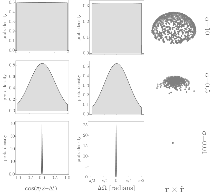
As mentioned in the earlier discussion on , an isotropic distribution is truly described by a uniform distribution in the cosine of the inclination angle. The same holds true if we want to produce an isotropic population of planets. However, as discussed before, it is the relative inclination angle that characterises coplanarity. For simplicity of notation, we denote the relative inclination angle as , where . A coplanar population is described by a highly compressed (approaching a Dirac Delta function) distribution centred on , or equivalently, and . On the other hand, we take a uniform distribution in the cosine of for an isotropic distribution, where we use the angle for consistency. Since a truncated normal has the flexibility to produce highly compressed, diffuse and even quasi-uniform distributions, we adopted this form in what follows. Accordingly, one may write that , where denotes a truncated normal distribution (with support from to and centered at ) and is the standard deviation, such that is consistent with a coplanar population and is consistent with an isotropic population. Finally, to convert between and (inclination of the planetary orbit measure with respect to the observer’s line of sight), we simply use the relationship , where is obtained from an isotropic distribution as discussed above.
For , it is again crucial to realize that it is the relative longitude of ascending node that characterises coplanarity. We denote the relative longitude of ascending node as (where ) and elect to also distribute the longitude of the ascending node of the planet following another truncated Gaussian. We limit ourselves to consider only prograde planets (planets orbiting in the same direction as the binary stars), which means we want to sample between and instead of the complete to range. To do so, we sample from a truncated Gaussian such that (with support from to and centered at ), where now by virtue of normalizing by we maintain the same truncation limits as with . Finally, we can convert between and using the relationship , where is obtained from an isotropic distribution as discussed above.
These two parameters, and , both describe the degree of non-coplanarity, but along different dimensions. For example, a coplanar population would correspond to and . In contrast, an isotropic population corresponds to and . In this way, and because of the carefully chosen parameterisation that maintains the same truncation limits, the degree of coplanarity can be encapsulated with just a single term, . To provide some context, the of all observed transiting circumbinary planets is (noting that is in fact a dimensionless quantity).
In Figure 2, we consider three representative values of : (corresponding to an isotropic population), (corresponding to an intermediate population between coplanar and isotropic), and (corresponding to a coplanar population). For each value of , we show the corresponding probability distributions for and . One can see that these, as well as the distribution of normal vectors on the globes, are consistent with the expected behaviours in limiting cases.
Now that all the relevant orbital parameters are established, we make the additional note that these parameters only set the initial configuration of a circumbinary planet system. They are by no means constant and can evolve over time according to the dynamics of the system. This time-dependence of the orbital parameters is fully captured by our simulations.
We are now ready to generate a random circumbinary system. Because we are investigating the effect of changing , these systems are of course not representative of the underlying distribution, whose is not well-characterised. But the stellar masses and binary separations are designed to be quasi-representative (especially once we filter out unphysical systems in the next subsection).
We use the rebound package (Rein & Liu, 2012) to evolve the circumbinary system over a time span much longer than one Kepler observing window and record the number of transits over each epoch. Note that we do not distinguish between the two stars when counting transits. In practice, it is often possible to distinguish the identity of the star being transited - especially for since the depths become increasingly distinct (e.g. Doyle et al. 2011). However, the misaligned nature of our systems means that the impact parameters are also constantly changing, leading to V-shaped transits and variable depths even for U-shaped events due to limb darkening (Mandel & Agol, 2002). This complicates the process of flagging identities to each event and introduces the possibility of mis-labelled events. In contrast, we argue that the simple act of counting how many dips are present in the data is far less ambiguous and thus presents a more robust labelling system, at the expense of some compromise in information content. Of course, even here there is the potential for some degree of confusion due to overlapping transits, but broadly one should expect the number of dips to be interpretable in such cases (e.g. see Gillon et al. 2017).
2.3 Filtering the Synthesised Sequences
After generating and evolving each of the circumbinary systems, we are left with a sequence of integers that denotes the number of transits per epoch for each planet. Next, we impose several filters to ensure that we are left with systems that are both physically sensible and observable.
Among all the observed circumbinary planets, the shortest period is days (Kepler-47b; Orosz et al. 2012). Accordingly, we impose this as a constraint in our artificial circumbinary population and filter out all planets with periods shorter than 50 days.
We can only extract information from circumbinary planets that are observable to us. In what follows, an “observable” planet is defined to be one that undergoes at least two epochs with at least one transit in one Kepler observing window. Thus, we need to filter out all unobservable planets.
To determine if a planet is “observable” or not, we first calculate the number of epochs it undertakes during one Kepler window and denote it as . Then, we randomly extract a sub-sequence of length from the full transits per epoch sequence we obtained from our simulation. If this sub-sequence does not contain at least two non-zero entries, them we discard it because it would outwardly lack the two necessary to cross our threshold of being “observable”. We repeat this procedure for all possible sub-sequences with length and filter out all the unobservable sub-sequences.
For an isotropic circumbinary planet population, % of the systems passes through the filters mentioned above and contain at least one length sub-sequence that is “observable”. On the other hand, only % of the systems in a coplanar planet population contain observable sub-sequences. The fact that coplanar systems are less likely to be observable seems counter-intuitive, but we note that for a coplanar system to be observable, the inclination of its binary and planet orbit must be precisely aligned to the observer’s line of sight. On the other hand, since the inclination of the binary and planet orbit is not correlated in the isotropic case, the requirement for observable systems is less stringent.
2.4 A Prediction Algorithm Using Memory
Recall that the underlying question tackled in this section is - do the transits per epoch sequences of transiting misaligned circumbinary planets follow a pattern which is discernible from being purely random? The hypothesis of a stochastic sequence could be undermined if were possible to make predictions for the next number in a sequence. Even if the accuracy of said predictions are not perfect, the demonstrable ability to predict better than random would still establish that the sequence was not truly stochastic in nature. To this end, we introduce a simple algorithm for predicting the number of transits a circumbinary planet undergoes in a given epoch using information from the previous epochs (hence the name "memory slot“), and show that the predictive power of this algorithm is consistently better than random guesses, thus proving that the transit occurrences of circumbinary planets are non-random and tractable.
2.4.1 Training and Testing the Algorithm
We are working with a sequence of integers that denotes the number of transits per epoch for the planet, and we wish to be able to predict the value of any of the integers in the sequence.
Taking inspiration from context networks (e.g. Sandford et al. 2021), we postulate that there is memory in this sequence. In particular, we will use a two memory slot prediction algorithm (see Section 2.4.2 for further justification). That is, we use the and integer in the sequence to predict the integer.
To “learn” how the predictive model works, we divide the dataset of transits per epoch sequences for a population of circumbinary planets into two parts: 80% goes into a training set, and 20% goes into a validation set. To predict the integer in a sequence in the validation set, we first identify the two-integer sequence consisting of the and integer that precedes the prediction slot. Then, we look for this two-integer sequence in the training set. For each occurrence of this sequence, we record the integer that immediately follows. Finally, we predict the integer to be the integer that has the highest probability (i.e. modal outcome) of following the and integer sequence in the training set. We direct the reader to Figure 3 for a graphic decomposition of the procedure described above.

2.4.2 Why Two Memory Slots?
In our prediction algorithm, we are using the two preceding slots to inform our prediction. We have also tried using more or fewer slots. With one memory slot, the prediction power of our algorithm was found to modestly decrease, with accuracy dropping by up to 7% depending on the assumed value. With more than two memory slots, the prediction power is almost identical to that of using only two memory slots, with accuracy increasing by up to 3% depending on the assumed value.
This indicates that the “memory” of circumbinary transits is primarily contained in the two preceding slots. Further, it demonstrates that amongst the two preceding slots, the one that is immediately before the slot of interest contains a larger fraction of the “memory”. Thus, using a two memory slot prediction algorithm ensures that we obtain the maximum prediction power with the least effort.
2.5 Comparing the Performance of the Prediction Algorithm
With the predictive model defined, we next turn to a point of comparison. We consider two possible "benchmark" models to this end, which we introduce in what follows. Further, we introduce the important concept of "broken sequences".
It is straightforward to apply the memory slot prediction algorithm described in Section 2.4 to the validation set and measure the corresponding prediction accuracy. However, this prediction accuracy in isolation means very little since it remains unclear whether our model establishes non-randomness to the sequences. To better understand and contextualise this prediction accuracy, it is useful to compare it to a benchmark accuracy, derived using a "naive" algorithm (following Sandford et al. 2021).
We considered two possible benchmarks. The first is obtained using a simplistic algorithm: predict the mode of the dataset every time. In this way, the model simply predicts the same guess every time once “trained”. As a second model, we try taking the observed sequence and simply drawing a random choice from it as the “prediction” for the next epoch. We dub these benchmark models as the “modal” and “random” models. Our prediction algorithm can claim to have predictive power only if it can out-perform these benchmarks.
2.6 Broken (and Unbroken) Sequences
In considering the types of sequences that might be observed, one concern is that many sequences might be discarded by automated surveys as seemingly impossible. This is particularly poignant for misaligned circumbinary systems, since the binary star may not be eclipsing and thus its binary nature may not even be known beforehand. A sequence such as “1111” would appear clearly reasonable, even with large timing variations, as a likely single planet transiting a single star with some additional hidden perturber (e.g. see Nesvorný et al. 2012). A sequence such as “1121” would also be quite reasonable, with the “2” event possibly caused by a second longer period transiting planet or even an exomoon (e.g. Teachey & Kipping 2018) - which we note need not transit each epoch (Martin et al., 2019). However, a sequence such as “1101” is far more challenging to understand and apparently without precedent (although the lack of precedence may simply be a product of the fact that such sequences are unexpected and thus possibly rejected). With the “1121” case, we can cluster the transits within each epoch together and still draw a quasi linear ephemeris through the times of the clustered events, consistent with the exomoon hypothesis for example. But a “1101” sequence produces a sparse chain that cannot be represented by even a quasi linear ephemeris. We consider here that such sequences, which we dub “broken sequences”, may trip over many automated searches and could plausibly be absent in future catalogs.
We define “broken sequences” as those for which the time gap between observable epochs (i.e. non-zero numbers of transits) is not constant (and thus an “unbroken sequence” is the opposite case).
For example, a transits per epoch sequence of “1011” or “100101” corresponds to a broken system, and a sequence of “1211” or “10201” corresponds to an unbroken system. The fraction of simulations that generate broken sequences is thus an important parameter when considering the occurrence rate and completeness estimates, in cases where this feature would indeed negatively impact the detectability of such sequences in surveys.
We find that the ratio of broken to unbroken sequences is strongly affected by the coplanarity of the circumbinary population generated. Varying the governing parameter in Figure 4, we find a log-logistic type behaviour emerges. This reveals that for quasi-isotropic populations, some 30% of sequences may present broken sequences in Kepler-like observing windows. Accordingly, surveys designed to measure the occurrence rate and properties of transiting circumbinary planets need to either use algorithms capable of identifying broken sequences or correct their rates for this effect appropriately.
As noted, the fraction of broken systems versus curve in Figure 4 resembles a logistic function. This can be understood by the fact that at extreme values of , the distribution saturates to either perfectly isotropic or perfectly coplanar.
2.7 Aliased (and Unaliased) Sequences
Broken systems could potentially cause a survey to reject a system as unphysical, although this of course depends upon the search algorithms being utilised. A sequence such as “1101” could be plausibly reconstructed though and the correct period inferred. However, the broken sequence “1010001” would be challenging to assign the true period for without detailed modelling or additional information; in particular we only observe the 1’s and so thus the simplest assumption is that the underlying sequence is “1101”. In such a case, we would have assigned an orbital period which is twice as long as the true one - an aliased period. Of course, this aliasing issue can also arise on unbroken sequences, such as the sequence “10101”. Thus, when interpreting such systems, besides from dividing the sequences up between broken and unbroken, we can also delineate them between “aliased” and “unaliased”.
This aliasing is important to our predictive model because it effectively transforms sequences like “1010001” “1101”, which will clearly influence the training and validation of our proposed algorithm. However, if the true period were known, perhaps through detailed modeling or additional observations such as radial velocity measurements, then this transformation would not occur and we could use our algorithm without modification.
As with broken sequences, the ratio of aliased and unaliased sequences exhibits a log-logistic type behaviour as we vary the governing parameter in Figure 4. For quasi-isotropic populations, more than a quarter of the sequences are aliased. This not only affects the training and validation of our proposed algorithm, but also implies that extra caution needs to be applied when assigning a period to observed transiting circumbinary planets.

2.8 Results
To summarise, we have proposed a simple predictive model for the number of transits per epoch based on the previous two epochs. In addition, we have proposed two benchmark predictive models that simply exploit the ensemble statistics rather than the last two epochs, one that always returns the mode and one that chooses a random sample from the list. In the results that follow, we always compare the performance of our full predictive model to these simpler two as a benchmark.
Further, we note that observed sequences can be delineated in two different ways. First, a sequence is “broken” if a quasi linear ephemeris cannot explained even the clustered sequence of transits (otherwise its unbroken). Such cases could potentially be missed by detection algorithms and thus deserve special consideration. Second, a sequence could lead one to assign an aliased period for the planet rather than the true one. In this way systems can be broken or unbroken, and also aliased or unaliased.
In evaluating the performance of our predictive model against the benchmark models, there are thus a total of 4 different scenarios that could be considered
-
A]
Broken+unbroken sequences, where the true period is correctly assigned.
-
B]
Broken+unbroken sequences, where the apparent period is assigned (which may be aliased).
-
C]
Unbroken sequences only, where the true period is correctly assigned.
-
D]
Unbroken sequences only, where the apparent period is assigned (which may be aliased).
For each of these four scenarios, we start from the transits per epoch sequences obtained from generating and evolving populations of circumbinary planets as prescribed in Section 2.2. Then we filter out the broken sequences and transform the aliased sequences to reflect the apparent period when necessary. The code we used to treat each of the four scenarios is made publicly available at this URL.
For each of the four scenarios, we compare the performance of our predictive model with the two benchmark models described in Section 2.5. Our results are summarised in Tables 1, 2, 3, and 4.
| frequency of 0/epoch | frequency of 1/epoch | frequency of 2/epoch | frequency of 3/epoch | frequency of 4+/epoch | two memory slot accuracy | modal benchmark accuracy | random benchmark accuracy | |
|---|---|---|---|---|---|---|---|---|
| 10 | 80.4% | 18.6% | 0.953% | 0.030% | 0% | 81.3% | 80.4% (0) | 64.4% |
| 3 | 79.8% | 19.1% | 1.10% | 0.063% | 0% | 80.7% | 79.8% (0) | 63.3% |
| 1 | 79.5% | 19.4% | 1.08% | 0.014% | 0% | 80.4% | 79.5% (0) | 62.2% |
| 0.5 | 78.3% | 19.7% | 1.82% | 0.126% | 0% | 80.7% | 78.3% (0) | 61.5% |
| 0.2 | 73.5% | 22.8% | 3.14% | 0.565% | 0.079% | 78.7% | 73.5% (0) | 54.4% |
| 0.1 | 66.5% | 26.9% | 5.75% | 0.626% | 0.179% | 78.2% | 66.5% (0) | 45.9% |
| 0.03 | 43.6% | 36.3% | 18.1% | 1.37% | 0.562% | 77.5% | 43.6% (0) | 35.3% |
| 0.01 | 26.8% | 41.4% | 26.1% | 4.28% | 1.38% | 81.9% | 41.4% (1) | 31.7% |
| 0.003 | 9.25% | 53.2% | 32.6% | 2.95% | 2.01% | 87.2% | 53.2% (1) | 39.4% |
| 0.001 | 2.46% | 55.1% | 36.7% | 4.21% | 2.24% | 89.7% | 55.1% (1) | 43.9% |
| 0.0001 | 1.70% | 44.7% | 44.5% | 5.09% | 3.25% | 90.5% | 44.7% (1) | 40.0% |
| frequency of 0/epoch | frequency of 1/epoch | frequency of 2/epoch | frequency of 3/epoch | frequency of 4+/epoch | two memory slot accuracy | modal benchmark accuracy | random benchmark accuracy | |
|---|---|---|---|---|---|---|---|---|
| 10 | 72.1% | 26.4% | 1.41% | 0.017% | 0% | 77.7% | 72.1% (0) | 49.8% |
| 3 | 72.0% | 26.9% | 1.46% | 0.180% | 0% | 77.8% | 72.0% (0) | 49.6% |
| 1 | 71.5% | 26.7% | 1.78% | 0.004% | 0% | 77.6% | 71.5% (0) | 50.5% |
| 0.5 | 72.3% | 25.4% | 2.18% | 0.150% | 0.013% | 78.9% | 72.3% (0) | 51.6% |
| 0.2 | 69.5% | 26.5% | 3.53% | 0.479% | 0.050% | 79.5% | 69.5% (0) | 48.4% |
| 0.1 | 64.4% | 28.4% | 6.41% | 0.593% | 0.241% | 79.1% | 64.4% (0) | 43.7% |
| 0.03 | 46.0% | 34.9% | 17.4% | 1.31% | 0.432% | 79.2% | 46.0% (0) | 34.0% |
| 0.01 | 23.5% | 43.4% | 26.7% | 4.54% | 1.83% | 83.2% | 43.4% (1) | 31.9% |
| 0.003 | 8.32% | 51.3% | 35.1% | 2.96% | 2.32% | 89.6% | 51.3% (1) | 38.9% |
| 0.001 | 2.06% | 56.8% | 35.4% | 3.72% | 2.04% | 91.4% | 56.8% (1) | 45.9% |
| 0.0001 | 1.58% | 42.7% | 46.8% | 5.36% | 3.56% | 91.8% | 46.8% (2) | 41.1% |
| frequency of 0/epoch | frequency of 1/epoch | frequency of 2/epoch | frequency of 3/epoch | frequency of 4+/epoch | two memory slot accuracy | modal benchmark accuracy | random benchmark accuracy | |
|---|---|---|---|---|---|---|---|---|
| 10 | 83.0% | 15.7% | 1.25% | 0.057% | 0% | 84.8% | 83.0% (0) | 66.1% |
| 3 | 82.4% | 16.5% | 0.943% | 0.119% | 0% | 84.2% | 82.4% (0) | 64.7% |
| 1 | 82.3% | 16.6% | 1.07% | 0.011% | 0% | 84.2% | 82.3% (0) | 64.8% |
| 0.5 | 82.8% | 15.9% | 1.23% | 0.087% | 0% | 85.0% | 82.8% (0) | 64.4% |
| 0.2 | 75.7% | 20.7% | 3.10% | 0.513% | 0.048% | 82.8% | 75.7% (0) | 54.7% |
| 0.1 | 66.9% | 25.3% | 6.78% | 0.895% | 0.158% | 81.4% | 66.9% (0) | 45.1% |
| 0.03 | 45.3% | 35.5% | 17.4% | 1.32% | 0.537% | 80.9% | 45.3% (0) | 34.0% |
| 0.01 | 24.9% | 39.6% | 26.4% | 6.70% | 2.32% | 85.9% | 39.6% (1) | 30.9% |
| 0.003 | 5.32% | 54.2% | 35.2% | 3.19% | 2.13% | 91.9% | 54.2% (1) | 42.0% |
| 0.001 | 1.60% | 52.6% | 40.0% | 4.88% | 2.38% | 91.6% | 52.6% (1) | 43.6% |
| 0.0001 | 0.141% | 43.1% | 47.5% | 4.87% | 3.41% | 92.6% | 47.5% (2) | 40.3% |
| frequency of 0/epoch | frequency of 1/epoch | frequency of 2/epoch | frequency of 3/epoch | frequency of 4+/epoch | two memory slot accuracy | modal benchmark accuracy | random benchmark accuracy | |
|---|---|---|---|---|---|---|---|---|
| 10 | 0% | 94.1% | 5.89% | 0% | 0.033% | 83.8% | 94.1% (1) | 90.0% |
| 3 | 0% | 95.0% | 4.52% | 0.439% | 0% | 87.2% | 95.0% (1) | 91.0% |
| 1 | 0% | 94.3% | 5.69% | 0% | 0% | 91.2% | 94.3% (1) | 90.5% |
| 0.5 | 0% | 91.9% | 7.42% | 0.634% | 0% | 85.0% | 91.9% (1) | 88.2% |
| 0.2 | 0% | 86.3% | 11.7% | 1.74% | 0.225% | 81.4% | 86.3% (1) | 78.9% |
| 0.1 | 0% | 77.5% | 19.8% | 2.62% | 0.119% | 78.3% | 77.5% (1) | 67.4% |
| 0.03 | 0% | 63.6% | 33.2% | 2.31% | 0.838% | 75.3% | 63.6% (1) | 55.3% |
| 0.01 | 0% | 59.6% | 35.2% | 2.91% | 2.26% | 87.6% | 54.6% (1) | 44.6% |
| 0.003 | 0% | 55.8% | 38.9% | 2.88% | 2.43% | 94.7% | 55.8% (1) | 45.0% |
| 0.001 | 0% | 56.2% | 36.4% | 4.46% | 2.92% | 92.6% | 57.2% (1) | 47.1% |
| 0.0001 | 0% | 43.9% | 47.6% | 5.23% | 3.30% | 91.7% | 47.6% (2) | 41.0% |
2.9 Interpreting the results
The results from this exercise reveal several important insights. First, the “random” version of the benchmark algorithm performs worse than the “modal” version for isotropic distributions, but the accuracies of the two benchmarks converge as we approach the coplanar distributions. For isotropic cases, the large of number of zeros clearly favours the modal method but as the sequences become more varied, the two methods converge in accuracy.
However, as a second key observation, we note that our two memory slot predictions almost always out-perform either benchmark. The only exception is in scenario D for the highly isotropic cases, where the modal case wins out. We note that the number of one’s is exceptionally high in this regime, reaching 94%, and thus the modal algorithm achieves excellent accuracy purely as a result of the monotonous nature of the sequences. For near coplanar cases, the two memory slot method reaches an accuracy of % where as the benchmark methods cannot do better than %.
As a result of this second observation, we can arrive at a conclusion concerning the original motivation behind this section. The number of transits per epoch for misaligned (or aligned) circumbinary transiting planets does not follow a purely random sequence and can be effectively predicted. As before, we emphasise that our prediction algorithm is not optimal and encourage work to develop improved iterations.
3 Transit Number Distribution vs. Inclination
We have seen how our parameter, which describes the degree of coplanarity of a population of systems, has a strong influence on the transit sequences that result. Of course, this analysis comes from a position of population synthesis where we know the true value (because we chose it). This raises the question as to how the inverse operation might proceed, to take an observed population and infer .
Already we have seen that there is a relationship between and the distribution of transits per epoch counts, reflected through the results shown in Section 2.8. This provides a pathway to potentially inferring the underlying alignment distribution by examining the distribution of transit counts.
Intuitively, this makes sense if we consider the extreme cases: for a perfectly coplanar circumbinary population, the observable planets almost always undergo at least one transit in per epoch In a perfectly isotropic circumbinary population, however, we would expect transits to be more sporadic (see Figure 1).
To go further than this simple intuition, we proceed by investigating the resulting transit counts distribution as a function of the assumed distribution. Sampling across a grid allows us to determine intermediate cases through an appropriate interpolation, and thus define a generalised model.
3.1 Transit Number Distribution at Selected Values of
As before, we generate and evolve populations of circumbinary planets as described in Section 2.2 and apply the filters described in Section 2.3. Furthermore, we do not assume prior knowledge of the planetary period, and thus sequences filled with many zeros (that can be explained by longer, aliased periods) are transformed with our aliasing transformation prescription (see Section 2.7).
The results are shown in Table 1 - 4 for each of the four scenarios described in Section 2.8. Scenarios B and D are particularly important, since they correspond to the case where one is simply tallying transits/epoch and is not equipped with special knowledge of the true period (which we consider to be the typical case in an automated survey). Scenarios B and D recall are distinct as to whether broken systems are included (B, yes; D, no) which is dependent upon the details of the search algorithm in question.
The results reveal how coplanar systems are indeed dominated by epochs with transits, as expected, but highly misaligned systems are far more sporadic. For isotropic distributions, we find that of the non-zero events, over % produce single transits. With such a high fraction of single-transit epochs, there is clearly a danger in such systems being misclassified as planets orbiting single stars - especially for scenario D where broken systems are discarded in the first place. Timing variations would of course also be present here but those could be interpretable as planet-planet interactions. In addition, such systems will exhibit depth variations for . This suggests that it may be useful to survey the existing catalog of planets ostensibly orbiting single stars to see if their depth and timing variations might also be consistent with a misaligned circumbinary scenario.
3.2 The Relationship between Transit Numbers and
In practice, one might conceive that inference of from a population of circumbinary planets would proceed through a full consideration of the transit shapes, durations, timing, etc to derive individual system posteriors, and then these would be fed into a population inference framework, such as hierarchical Bayesian modelling (e.g. see Hogg et al. 2010; Chen & Kipping 2017). Indeed, population level analyses of the alignment of circumbinary transits have already been published, such as that of Li et al. (2016) who favour a nearly coplanar population. However, given the poor sensitivity to misaligned systems with current methods (Martin, 2018), the influence of selection bias may be driving this.
In what follows, we seek a simplified description for inferring that depends on the simple and well-defined metric of transit counts per epoch. Whilst surely more precise inferences of the inclination distribution could be inferred by leveraging the finer grained information encoded in the light curve, this metric is attractive for its simplicity, enabling a relatively straight-forward inference procedure.
To accomplish this, we first need an interpolating function of the grid of results presented earlier. In what follows, we use the results from Scenario D, as the likely typical scenario, but the below can be repeated for any of the other scenarios following the same prescription. Note that in this scenario, broken sequences are removed and the remaining unbroken sequences undergo an aliasing transform. This means that there are no zeros in the final sequences.
As was found in Figure 4, we find that logistic functions work well in this problem when the independent variable is . This is because at extreme values of , the distribution saturates to either perfectly isotropic or perfectly coplanar. Thus, we regressed logistic function fits to the 4 non-zero columns in the middle panel of Table 4. Additionally, we impose the constraint that probabilities must be greater than 0, less than 1, and sum to 1. To impose the “sum to unity” constraint, we choose to fit columns 3, 4, 5 of the middle panel first under the constraint that they sum to less than unity, then calculate the value of column 2 by hand222We also tried other combinations of these but found this to provide the best match to our simulation results..
The resulting fits are shown in Figure 5, where one can see the close agreement achieved between the logistic functions and the simulation results. Note that even for column 2 where we manually computed the values instead of directly optimising the fit, the errors are still quite small, which validates our fitting strategy.

The logistic function fits are as follows, where is the fraction of epochs exhibiting transits:
| (3) | ||||
| (4) | ||||
| (5) |
and by definition
| (6) |
Naturally, the above could be easily repeated for the other scenarios, where we note that one would need to include an function to account for zero-transit epochs.
3.3 Constraining the Inclination Distribution
Consider that we have observed transit epochs of distinct transiting circumbinary planets. The objects form a population, for example a group of known circumbinary systems with similar stellar parameters. Let us assume that each member of the population has a unique and value, and that that the ensemble of these values can be approximately described by the truncated normal distributions posited in Section 2.2 and depicted in Figure 2. In this way, each object has a unique orbital alignment but the population is characterised by a single parameter - .
From the sample of epochs, we can count the number of cases where just a single transit is observed, , or two transits, , etc. Defining as the number of of 4+ transits, we expect . Note that, in general, is not directly observed, but rather inferred from the lack of a transit and an inferred ephemeris. However, in our case of assuming scenario D, it is not possible to have a zero-transit epoch as discussed earlier so we can discard and define . Equipped with the data , we might ask - what is the allowed range for that can accommodate these observations?
To make this inference, it is necessary to first define a likelihood function, . The likelihood of obtaining the data , given a choice of , can be expressed as a multinomial probability mass function, since the problem is discretised:
| (7) |
Since the binomial term in the above is simply a constant for a given set of data, , the objective function for inference can be expressed as
| (8) |
The likelihood function is typically a monotonic function of and thus a central value of is not well-defined (see Figure 6). Instead, it is typically more useful to state that tends toward the coplanar/isotropic asymptote, and then assign a statistical upper/lower limit on parameter, respectively.
To show an example, we set and sampled epochs to produce the fake data set . Once again, we emphasise that because we are working in scenario D, there are no zero transit epochs by construction. The likelihood function is shown in the top panel of Figure 6, plateaus at small and suggests a nearly coplanar solution. Credible intervals for 68.3% and 95.5% are shaded in hatch and cross-hatch respectively, which are found to be consistent with the injected truth. The exercise was repeated for and produced another self-consistent recovery (see lower panel of Figure 6), despite the fact the likelihood function flips over and favours an isotropic solution here.
The inference model here is simplistic and could surely be improved by leveraging other information within each epoch (e.g. transit durations), labelling the transits by star and considering alternative population models beyond a truncated normal. But our simple demonstration establishes that transit sequences already provide constraining power on the population’s inclination distribution and the problem is tractable.

4 Discussion
In this work, we have considered the possibility that there exists a population of misaligned circumbinary transiting planets and explored the observational consequences. In particular, we have explored the chronological integer sequences of the number of transits per epoch. Transit flagging is possible through visual inspection (e.g. Eisner et al. 2021) or automated detection, even in the case of arbitrarily shaped dips Wheeler & Kipping (2019), and the number of transits per epoch would simply be the temporal clusterings of these events. Thus, we expect that the number of dips occurring in each epoch is a readily observable quantity, available without significant photodynamical analysis (e.g. Doyle et al. 2011). In this context though, misaligned circumbinaries present ostensibly foreign sequences when viewed from the familiar perspective of planets orbiting single stars. We have shown that zero, one, two or three transits per epoch are not atypical, due to the possibility of missing the stars and the binary’s inner motion. These sequences are so seemingly strange to conventional search algorithms that they risk being missed altogether (Martin, 2018), and thus our work lays out the expected frequency, patterns and applicability of them.
We have produced synthetic populations of such transit sequences under various assumptions about the inclination distribution. However, the corresponding sequences depend upon the details of the detection algorithms that will ultimately seek them. For example, if sequences include zero-transit events, it may appear seemingly impossible to draw a quasi-linear ephemeris through the data even after clustering them into epochs - so-called “broken” sequences (e.g. “1101”). This are the tell-tale signature of a misaligned circumbinary but of course few algorithms are designed to accommodate the possibility of missing epochs like this, and thus they may not be ever reported due to detection bias.
We also show how even if the broken sequences can be detected, the naively inferred period (maximum period which can explain the non-zero epochs) may be wrong if the sequences are spaced with quasi-regular zero’s. We dub these “aliased sequences”. For example, the sequence “10101” would be naively observed as just “111” assuming the period is twice that of reality. That example represents an unbroken sequence, but the problem is of course exacerbated for unbroken sequences. This aliasing issue could be resolved using photodynamics, radial velocity or astrometry analysis but such features are rarely integral part of how transit algorithms function.
We show that for nearly isotropic distributions of the binary misalignment angles, zero-transit epochs dominate. With % of epochs being a zero, our work establishes that any search algorithm aiming for completeness will have to account for this possibility. Yet more, the occurrence of two or more transits per epoch, the typical giveaway that one is looking at a transiting circumbinary, is quite rare - occurring in less than 1% of epochs. Thus, highly misaligned circumbinary systems may be hiding in plain sight in our data sets, producing sporadic single transits of varying depths, durations and irregular spacing.
On the more optimistic side, we have established that these sequences will not appear as purely random integer chains, and that even two epochs can accurately predict the third. In principle then, a successful prediction of the next epoch could establish the system is consistent with a circumbinary. However, our algorithm is trained on cases where the underlying inclination distribution is known (e.g. isotropic) and thus in practice applying this to real data would involve even sifting through a selection of possible inclination distributions, or modifying as needed. As emphasised throughout, we do not claim this algorithm is in any way optimal, but is rather used to simply demonstrate the sequences are non-random in nature (and thus could surely be improved upon).
Finally, we have shown that these sequences encode information about the inclination distribution, allowing us to in principle test whether a given set of transit sequences are consistent with an isotropic or coplanar distribution. That information could of course aid in the prediction issue mentioned earlier. But, as before, the inference could surely be improved upon by leveraging a full photodyanamical analysis - the point here is really just to demonstrate that information is encoded with it and is accessible with even a simple model.
Together, our work highlights the challenges and opportunities that misaligned transiting circumbinary systems present, taking the observational view that we often know little more than the timing of transits producing strange patterns (e.g, Rappaport et al. 2019). As transit surveys grow in scope and size, the need to consider such systems will likely similarly grow.
Acknowledgements
We thank the anonymous reviewers for their constructive feedback, which significantly improved this work. This paper made use of data collected by the Kepler mission and accessed from the Data Release 25 (DR25) Kepler Input Catalog queried using the Mikulski Archive for Space Telescopes (MAST). Funding for the Kepler mission is provided by the NASA Science Mission directorate. We also gratefully acknowledge the developers of the following software packages which made this work possible: rebound (Rein & Liu, 2012), astropy (Astropy Collaboration et al., 2013), numpy (van der Walt et al., 2011; Harris et al., 2020), scipy (Virtanen et al., 2020), and matplotlib (Hunter, 2007). Simulations in this paper made use of Columbia’s Habanero High Performance Computation Cluster.
We thank the Cool Worlds Lab team members for useful discussions and comments. This work was enabled thanks to supporters of the Cool Worlds Lab, including Mark Sloan, Douglas Daughaday, Andrew Jones, Elena West, Tristan Zajonc, Chuck Wolfred, Lasse Skov, Graeme Benson, Alex de Vaal, Mark Elliott, Methven Forbes, Stephen Lee, Zachary Danielson, Chad Souter, Marcus Gillette, Tina Jeffcoat, Jason Rockett, Scott Hannum, Tom Donkin, Andrew Schoen, Jacob Black, Reza Ramezankhani, Steven Marks, Philip Masterson, Gary Canterbury, Nicholas Gebben, Joseph Alexander & Mike Hedlund.
Data Availability
The code we used to generate and evolve circumbinary planet populations and the data we obtained is made publicly available at this URL.
References
- Armstrong et al. (2014) Armstrong D. J., Osborn H. P., Brown D. J. A., Faedi F., Gómez Maqueo Chew Y., Martin D. V., Pollacco D., Udry S., 2014, MNRAS, 444, 1873
- Astropy Collaboration et al. (2013) Astropy Collaboration et al., 2013, A&A, 558, A33
- Carter & Agol (2013) Carter J. A., Agol E., 2013, ApJ, 765, 132
- Chapman et al. (1992) Chapman S., et al., 1992, Nature, 359, 207–210
- Chen & Kipping (2017) Chen J., Kipping D., 2017, ApJ, 834, 17
- Czekala et al. (2019) Czekala I., Chiang E., Andrews S. M., Jensen E. L. N., Torres G., Wilner D. J., Stassun K. G., Macintosh B., 2019, ApJ, 883, 22
- Demircan & Kahraman (1991) Demircan O., Kahraman G., 1991, Ap&SS, 181, 313
- Doyle et al. (2011) Doyle L. R., et al., 2011, Science, 333, 1602
- Dvorak (1986) Dvorak R., 1986, A&A, 167, 379
- Eisner et al. (2021) Eisner N. L., et al., 2021, MNRAS, 501, 4669
- Gillon et al. (2017) Gillon M., et al., 2017, Nature, 542, 456
- Hamers et al. (2016) Hamers A. S., Perets H. B., Portegies Zwart S. F., 2016, MNRAS, 455, 3180
- Harris et al. (2020) Harris C. R., et al., 2020, Nature, 585, 357–362
- Hatzes et al. (2003) Hatzes A. P., Cochran W. D., Endl M., McArthur B., Paulson D. B., Walker G. A. H., Campbell B., Yang S., 2003, ApJ, 599, 1383
- Hogg et al. (2010) Hogg D. W., Myers A. D., Bovy J., 2010, ApJ, 725, 2166
- Holman & Wiegert (1998) Holman M. J., Wiegert P. A., 1998, Astron.J., 117, 621
- Hunter (2007) Hunter J. D., 2007, Computing in Science and Engineering, 9, 90
- Karttunen et al. (1994) Karttunen H., Kröger P., Oja H., Poutanen M., Donner K. J., 1994, Binary Stars and Stellar Masses. Springer Berlin Heidelberg, Berlin, Heidelberg, pp 247–255, doi:10.1007/978-3-662-11794-1_10, https://doi.org/10.1007/978-3-662-11794-1_10
- Klagyivik et al. (2017) Klagyivik P., Deeg H. J., Cabrera J., Csizmadia S., Almenara J. M., 2017, A&A, 602, A117
- Kovács et al. (2002) Kovács G., Zucker S., Mazeh T., 2002, A&A, 391, 369
- Kraus et al. (2016) Kraus A. L., Ireland M. J., Huber D., Mann A. W., Dupuy T. J., 2016, AJ, 152, 8
- Lam & Kipping (2018) Lam C., Kipping D., 2018, Monthly Notices of the Royal Astronomical Society, 476, 5692–5697
- Li et al. (2016) Li G., Holman M. J., Tao M., 2016, ApJ, 831, 96
- Mandel & Agol (2002) Mandel K., Agol E., 2002, ApJ, 580, L171
- Martin (2018) Martin D. V., 2018, Populations of Planets in Multiple Star Systems. p. 156, doi:10.1007/978-3-319-55333-7_156
- Martin & Triaud (2014) Martin D. V., Triaud A. H. M. J., 2014, A&A, 570, A91
- Martin et al. (2019) Martin D. V., Fabrycky D. C., Montet B. T., 2019, ApJ, 875, L25
- Muñoz & Lai (2015) Muñoz D. J., Lai D., 2015, Proceedings of the National Academy of Science, 112, 9264
- Murray & Correia (2010) Murray C. D., Correia A. C. M., 2010, Keplerian Orbits and Dynamics of Exoplanets. pp 15–23
- Nesvorný et al. (2012) Nesvorný D., Kipping D. M., Buchhave L. A., Bakos G. Á., Hartman J., Schmitt A. R., 2012, Science, 336, 1133
- Orosz et al. (2012) Orosz J. A., et al., 2012, Science, 337, 1511
- Parker & Reggiani (2013) Parker R. J., Reggiani M. M., 2013, MNRAS
- Pringle (1989) Pringle J. E., 1989, MNRAS, 239, 361–370
- Quarles et al. (2018) Quarles B., Satyal S., Kostov V., Kaib N., Haghighipour N., 2018, ApJ, 856, 150
- Raghavan et al. (2010) Raghavan D., et al., 2010, The Astrophysical Journal Supplement Series, 190, 1
- Rappaport et al. (2019) Rappaport S., et al., 2019, MNRAS, 488, 2455
- Rein & Liu (2012) Rein H., Liu S. F., 2012, A&A, 537, A128
- Sandford et al. (2021) Sandford E., Kipping D., Collins M., 2021, MNRAS, 505, 2224
- Santerne et al. (2014) Santerne A., et al., 2014, A&A, 571, A37
- Teachey & Kipping (2018) Teachey A., Kipping D. M., 2018, Science Advances, 4, eaav1784
- Thebault & Haghighipour (2015) Thebault P., Haghighipour N., 2015, Planet Formation in Binaries. pp 309–340, doi:10.1007/978-3-662-45052-9_13
- Tohline (2002) Tohline J. E., 2002, ARA&A, 40, 349
- Virtanen et al. (2020) Virtanen P., et al., 2020, Nature Methods, 17, 261
- Welsh et al. (2012a) Welsh W. F., Orosz J. A., Carter J. A., Fabrycky D. C., 2012a, Proceedings of the International Astronomical Union, 8, 125–132
- Welsh et al. (2012b) Welsh W. F., et al., 2012b, Nature, 481, 475
- Wheeler & Kipping (2019) Wheeler A., Kipping D., 2019, MNRAS, 485, 5498
- Windemuth et al. (2019) Windemuth D., Agol E., Carter J., Ford E. B., Haghighipour N., Orosz J. A., Welsh W. F., 2019, MNRAS, 490, 1313
- Xu & Lai (2016) Xu W., Lai D., 2016, MNRAS, 459, 2925
- van der Walt et al. (2011) van der Walt S., Colbert S. C., Varoquaux G., 2011, Computing in Science Engineering, 13, 22