The no–hair theorems at work in M87^∗

It has recently been proven 2024arXiv241108686I that a simple perturbative calculation to the first post–Newtonian (1pN) order of the Lense–Thirring (LT) effect on the orbit of a test particle moving about a massive spinning object is able to reproduce, both qualitatively and quantitatively, several features of the jet precession in the supermassive black hole (SMBH) M87^∗ recently measured with the Very Long Baseline Interferometry (VLBI) technique 2023Natur.621..711C . Aim of this paper is to show that, actually, also the mass quadrupole moment¹¹1The possible impact of electric charge was recently investigated 2024arXiv241107481M in the framework of the Kerr–Newman metric 1965JMP…..6..915N ; 1965JMP…..6..918N as well. of M87^∗, neglected so far in the literature, should be fully taken into account in the dynamics of the accretion disk, assumed tightly coupled with the jet 2013Sci…339…49M ; 2018MNRAS.474L..81L ; 2024arXiv241010965C . The imprints of the precession of the latter on the SMBH-accretion disk system was recently investigated in 2024arXiv241010965C . The introduction of the hole’s quadrupole does not spoil the agreement between the perturbative analytical calculation and the characteristics measured in 2023Natur.621..711C , yielding to different allowed regions for the hole’s spin parameter and the radius of the effective circular orbit modeling the precessing disk. As a result, the celebrated “no–hair” (NH) theorems 1967PhRv..164.1776I ; 1971PhRvL..26..331C ; 1975PhRvL..34..905R receive a strong support.

According to the latter ones, the mass and the spin moments $\mathcal{M}^{\ell}$ and $\mathcal{J}^{\ell}$ of degree $\ell$ of a rotating BH 1970Natur.226…64B , whose external spacetime is described by the Kerr metric 1963PhRvL..11..237K ; 2015CQGra..32l4006T , are connected by the relation

$$\mathcal{M}^{\ell}+i\,\mathcal{J}^{\ell}=M\left(i\,\frac{J}{cM}\right)^{\ell},$$

(1)

where $i:=\sqrt{-1}$ is the imaginary unit, $c$ is the speed of light, and $M$ and $J$ are the hole’s mass and spin angular momentum, respectively. From Equation (\T@refnohair), it turns out that the odd mass moments and even spin moments are identically zero. In particular, the hole’s mass moment $\mathcal{M}^{0}$ of degree $\ell=0$ is its mass, while its spin dipole moment $\mathcal{J}$ of degree $\ell=1$ is its spin angular momentum. For a Kerr BH, it is 1986bhwd.book…..S

$$J=\chi\frac{M^{2}G}{c},\,\left|\chi\right|\leq 1,$$

(2)

where $G$ is the Newtonian constant of gravitation. Furthermore, the mass quadrupole moment $\mathcal{M}^{2}$ of degree $\ell=2$, renamed $Q_{2}$, is

$$Q_{2}=-\frac{J^{2}}{c^{2}M}.$$

(3)

If $\left|\chi\right|>1$, a naked singularity 1973CMaPh..34..135Y ; 1991PhRvL..66..994S without a horizon would occur, implying the possibility of causality violations because of closed timelike curves. Although not yet proven, the cosmic censorship conjecture 1999JApA…20..233P ; 2002GReGr..34.1141P states that naked singularities may not be formed via the gravitational collapse of a material body. The dimensionless parameter $\chi$ can also be viewed as the second characteristic length²²2Sometimes, the symbol $a$ is used for $J/\left(cM\right)$ itself, in which case it is dimensionally a length. $J/\left(cM\right)$ occurring in the Kerr metric 1963PhRvL..11..237K ; 2015CQGra..32l4006T measured in units of the gravitational radius $R_{\mathrm{g}}:=GM/c^{2}$. In BH studies, $\chi$ is often denoted with $a$, which is the same symbol usually adopted in celestial mechanics and astrodynamics to denote the semimajor axis of a generally elliptical orbit of a test particle.

The organization of the paper is as follows. Section \T@refsect:model offers a review of the perturbative analytical model of the LT and mass quadrupole effects, expressed in terms of the both the Keplerian orbital elements and in vectorial form, for a generic orientation of the primary’s spin axis in space. In Section \T@refsect:application, the previous results are successfully applied to the measured precession of the jet of M87^∗, assumed strongly coupled with that of the accretion disk. Section \T@reffine summarizes the findings and offers conclusions.

The inclination $I$ and the longitude of the ascending node $\mathit{\Omega}$ define the orientation of the orbital plane in space. Their LT rates of change averaged over one orbital revolution and valid for an arbitrary orientation of the primary’s spin axis $\boldsymbol{\hat{k}}$ turn out to be

	$\displaystyle\dot{I}^{\mathrm{LT}}$	$\displaystyle=\frac{2GJ\left(\boldsymbol{\hat{k}}\boldsymbol{\cdot}\boldsymbol{\hat{l}}\right)}{c^{2}a^{3}\left(1-e^{2}\right)^{3/2}},$		(4)
	$\displaystyle\dot{\mathit{\Omega}}^{\mathrm{LT}}$	$\displaystyle=\frac{2GJ\csc I\left(\boldsymbol{\hat{k}}\boldsymbol{\cdot}\boldsymbol{\hat{m}}\right)}{c^{2}a^{3}\left(1-e^{2}\right)^{3/2}},$		(5)

where, for a Kerr BH, $J$ is given by Equation (\T@refJei). Furthermore, $a$ and $e$ are the orbit’s semimajor axis and eccentricity, respectively. The unit vectors $\boldsymbol{\hat{l}}$ and $\boldsymbol{\hat{m}}$, which lie in the orbital plane and are mutually orthogonal, are defined as Sof89 ; 1991ercm.book…..B ; SoffelHan19 ; 2024gpno.book…..I

	$\displaystyle\boldsymbol{\hat{l}}$	$\displaystyle:=\left\{\cos\mathit{\Omega},\sin\mathit{\Omega},0\right\},$		(6)
	$\displaystyle\boldsymbol{\hat{m}}$	$\displaystyle:=\left\{-\cos I\sin\mathit{\Omega},\cos I\cos\Omega,\sin I\right\}.$		(7)

Equations (\T@refdotILT)–(\T@refdotOLT) were worked out with a perturbative calculation to the 1pN order by means of the equations for the rates of change of the Keplerian orbital elements in Gaussian or Lagrange form Sof89 ; 1991ercm.book…..B ; 2000ssd..book…..M ; 2003ASSL..293…..B ; 2005ormo.book…..R ; 2011rcms.book…..K ; 2014grav.book…..P ; SoffelHan19 ; 2024gpno.book…..I .

The mean rates of changes of the same orbital elements caused by the oblateness of a massive primary, valid for a generic orientation of $\boldsymbol{\hat{k}}$, can be calculated with the same approach obtaining 2024gpno.book…..I

	$\displaystyle\dot{I}^{Q_{2}}$	$\displaystyle=-\frac{3}{2}n_{\mathrm{K}}J_{2}\left(\frac{R}{p}\right)^{2}\left(\boldsymbol{\hat{k}}\boldsymbol{\cdot}\boldsymbol{\hat{h}}\right)\left(\boldsymbol{\hat{k}}\boldsymbol{\cdot}\boldsymbol{\hat{l}}\right),$		(8)
	$\displaystyle\dot{\mathit{\Omega}}^{Q_{2}}$	$\displaystyle=-\frac{3}{2}n_{\mathrm{K}}J_{2}\csc I\left(\frac{R}{p}\right)^{2}\left(\boldsymbol{\hat{k}}\boldsymbol{\cdot}\boldsymbol{\hat{h}}\right)\left(\boldsymbol{\hat{k}}\boldsymbol{\cdot}\boldsymbol{\hat{m}}\right).$		(9)

In Equations (\T@refdotIQ2)–(\T@refdotOQ2), $n_{\mathrm{K}}:=\sqrt{GM/a^{3}}$ is the Keplerian mean motion, $p:=a\left(1-e^{2}\right)$ is the semilatus rectum, the unit vector $\boldsymbol{\hat{h}}$, directed along the orbital angular momentum and orthogonal to both $\boldsymbol{\hat{l}}$ and $\boldsymbol{\hat{m}}$ in such a way that $\boldsymbol{\hat{l}}\boldsymbol{\times}\boldsymbol{\hat{m}}=\boldsymbol{\hat{h}}$ holds, is defined as Sof89 ; 1991ercm.book…..B ; SoffelHan19 ; 2024gpno.book…..I

$$\boldsymbol{\hat{h}}:=\left\{\sin I\sin\mathit{\Omega},-\sin I\cos\mathit{\Omega},\cos I\right\},$$

(10)

$R$ is the equatorial radius of the primary, and $J_{2}$ is its dimensionless mass quadrupole moment. The latter one must be expressed in terms of its dimensional counterpart $Q_{2}$ having dimensions of a mass times a length squared as

$$J_{2}:=-\frac{Q_{2}}{MR^{2}},$$

(11)

which, for a Kerr BH, is given by Equation (\T@refQ2).

The resulting NH orbital rates are

	$\displaystyle\dot{I}^{\mathrm{NH}}$	$\displaystyle=\dot{I}^{\mathrm{LT}}+\dot{I}^{Q_{2}},$		(12)
	$\displaystyle\dot{\mathit{\Omega}}^{\mathrm{NH}}$	$\displaystyle=\dot{\mathit{\Omega}}^{\mathrm{LT}}+\dot{\mathit{\Omega}}^{Q_{2}}.$		(13)

Equations (\T@refdotILT)–(\T@refacca) can be used to express the precession of the unit vector $\boldsymbol{\hat{h}}$ of the orbital angular momentum in a compact form as

$$\frac{{{\textrm{d}}}{\boldsymbol{\hat{h}}}}{{{\textrm{d}}}{t}}=\frac{\partial{\boldsymbol{\hat{h}}}}{\partial{I}}\,\dot{I}^{\mathrm{NH}}+\frac{\partial{\boldsymbol{\hat{h}}}}{\partial{\mathit{\Omega}}}\,\dot{\mathit{\Omega}}^{\mathrm{NH}}={\boldsymbol{\Omega}}_{\mathrm{d}}^{\mathrm{NH}}\boldsymbol{\times}\boldsymbol{\hat{h}}.$$

(14)

In it, the precession velocity vector ${\boldsymbol{\Omega}}^{\mathrm{NH}}_{\mathrm{d}}$ is

$${\boldsymbol{\Omega}}_{\mathrm{d}}^{\mathrm{NH}}={\boldsymbol{\Omega}}_{\mathrm{d}}^{\mathrm{LT}}+{\boldsymbol{\Omega}}_{\mathrm{d}}^{Q_{2}},$$

(15)

where

	$\displaystyle{\boldsymbol{\Omega}}_{\mathrm{d}}^{\mathrm{LT}}$	$\displaystyle=\frac{2GJ}{c^{2}a^{3}\left(1-e^{2}\right)^{3/2}}\boldsymbol{\hat{k}},$		(16)
	$\displaystyle{\boldsymbol{\Omega}}_{\mathrm{d}}^{Q_{2}}$	$\displaystyle=-\frac{3}{2}n_{\mathrm{K}}J_{2}\left(\frac{R}{p}\right)^{2}\left(\boldsymbol{\hat{k}}\boldsymbol{\cdot}\boldsymbol{\hat{h}}\right)\boldsymbol{\hat{k}}.$		(17)

From Equations (\T@refprecNH)–(\T@refprecQ2), it can be noted that the orbital angular momentum precesses around the primary’s spin axis. Such results are in agreement with 1974PhRvD..10.1340B ; 1975PhRvD..12..329B , where the term accounting also for the simultaneous precession of the Laplace–Runge–Lenz vector Gold80 ; Taff85 , of no interest here, was included in the total precessional velocity.

In the following, the spin axis of M87^∗ will be parameterized as

$$\boldsymbol{\hat{k}}=\left\{\sin\theta\sin\eta_{\mathrm{p}},-\sin\theta\cos\eta_{\mathrm{p}},\cos\theta\right\},$$

(18)

where 2023Natur.621..711C

	$\displaystyle\theta$	$\displaystyle=17.21^{\circ},$		(19)
	$\displaystyle\eta_{\mathrm{p}}$	$\displaystyle=288.47^{\circ}.$		(20)

By considering the total NH precession velocity, given by Equations (\T@refprecNH)–(\T@refprecQ2), as a function of $a^{\ast}$ and the effective radius $r_{0}$ of the precessing accretion disk, it is possible to plot its absolute value by imposing the condition that its graph is comprised within the upper an lower measured values of the absolute value of the measured precession velocity 2023Natur.621..711C

$$\left|\omega^{\mathrm{exp}}_{\mathrm{p}}\right|=0.56\pm 0.02\,\mathrm{rad\,yr}^{-1},$$

(21)

i.e.,

$$0.54\,\mathrm{rad\,yr}^{-1}\leq\left|\Omega_{\mathrm{d}}^{\mathrm{NH}}\left(a^{\ast},r_{0}\right)\right|\leq 0.58\,\mathrm{rad\,yr}^{-1}.$$

(22)

The sets of the values of $a^{\ast}$ and $r_{0}$ satisfying the condition of Equation (\T@refcondiz) form allowed regions in the $\left\{a^{\ast},r_{0}\right\}$ plane depicted in pale yellow in Figure \T@reffigure:allowed:tot.

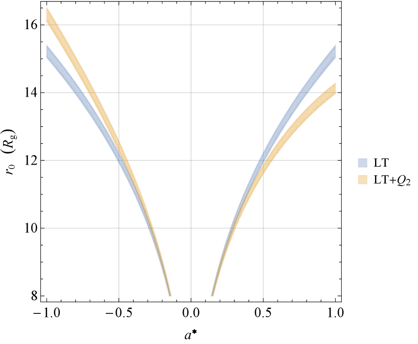In it, also the permitted regions obtained by considering solely the LT effect are shown in pale blue as well 2024arXiv241108686I . It turns out that both the LT and the $\mathrm{LT}+Q_{2}$ regions overlap in the no–rotation limit $\left|a^{\ast}\right|\rightarrow 0$, as expected. Instead, they separate when the hole’s spin parameter tends to unity. While both the allowed branches are equal and symmetric with respect to the $a^{\ast}=0$ axis in the LT–only case, the inclusion of the SMBH’s quadrupole breaks such a symmetry allowing for larger values of $r_{0}$ corresponding to the retrograde rotation of the hole ($a^{\ast}<0$) with respect to the prograde case ($a^{\ast}>0$). As a general feature, for prograde hole’s rotation, $Q_{2}$ generally tends to shrink the disk (right branches), while the opposite occurs for retrograde hole’s rotation (left branches) with respect to the LT–only scenario. The minimum physically admissible value for $r_{0}$ was taken from Figure 1 of 2024PhRvD.109b4029A which depicts the radius of the tilted³³3The tilt is with respect to the hole’s equator. innermost stable circular orbit (TISCO) for different values of the spin–orbit tilt angle, called $\psi_{\mathrm{jet}}$ in 2023Natur.621..711C (see below for more on it). It turns out that, for slightly tilted orbits as in the case of M87^∗ ($\psi^{\mathrm{M87^{\ast}}}_{\mathrm{jet}}\simeq 1.25^{\circ}$ 2023Natur.621..711C ), the radius of the TISCO is

	$\displaystyle r_{\mathrm{TISCO}}$	$\displaystyle\simeq 8R_{\mathrm{g}}\,\left(a^{\ast}\simeq-1\right),$		(23)
	$\displaystyle r_{\mathrm{TISCO}}$	$\displaystyle\simeq 2R_{\mathrm{g}}\,\left(a^{\ast}\simeq 1\right).$		(24)

Figure \T@reffigure:allowed_plus_minus shows two insets of Figure \T@reffigure:allowed:tot corresponding to $\left|a^{\ast}\right|\lesssim 1$, in agreement with most of the constraints on it existing in the literature 1998AJ….116.2237K ; 2008ApJ…676L.109W ; 2009ApJ…699..513L ; 2012Sci…338..355D ; 2017MNRAS.470..612F ; 2018MNRAS.479L..65S ; 2019ApJ…880L..26N ; 2019MNRAS.489.1197N ; 2020AnP…53200480G ; 2020MNRAS.492L..22T ; 2023Astro…2..141D .

In such regimes, the impact of $Q_{2}$ appears quite evident with respect to the case in which only the LT effect is taken into account.

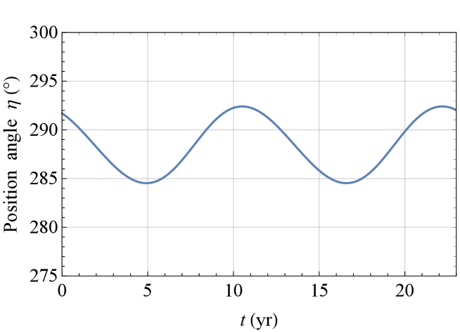
Figures \T@reffigure:etaphi_plus to \T@reffigure:etaphi_minus display the numerically integrated NH time series of the time–dependent angles $\eta\left(t\right)$ and $\phi\left(t\right)$ determining the orientation of the disk’s orbital angular momentum in space; in the language of celestial mechanics and astrodynamics, they correspond to the longitude of the ascending node $\mathit{\Omega}$ and the inclination $I$, respectively. Their signatures were theoretically obtained by simultaneously integrating the averaged equations for the rates of change of Equations (\T@refdotI)–(\T@refdotO) by adopting the values $a^{\ast}=+0.98,r_{0}=14.1\,R_{g}$ (Figure \T@reffigure:etaphi_plus) and $a^{\ast}=-0.95,r_{0}=16\,R_{g}$ (Figure \T@reffigure:etaphi_minus), contained in the pale yellow regions of the upper and lower panels of Figure \T@reffigure:allowed_plus_minus, respectively.

It can be noted that the NH prograde signatures displayed in Figure \T@reffigure:etaphi_plus agree well with their measured counterparts of Figure 2 $\boldsymbol{\left(\mathrm{b}\right)}$ and Extended Data Figure 4 of 2023Natur.621..711C , both qualitatively and quantitatively. It is not the case for the NH retrograde signals of Figure \T@reffigure:etaphi_minus which, if on the one hand, retain the same sizes of those in Figure 2 $\boldsymbol{\left(\mathrm{b}\right)}$ and Extended Data Figure 4 of 2023Natur.621..711C , on the other hand, appear to be out of phase with respect to the latter ones.

As far as the spin–orbit tilt angle $\psi_{\mathrm{jet}}$ is concerned, both its theoretically predicted value and its temporal evolution, calculated by integrating Equations (\T@refdotI)–(\T@refdotO) as before, do not change with respect to their LT–only counterparts, shown in Figure 5 of 2024arXiv241108686I , which were already found to be in agreement with their measured values.

The no–hair theorems are fully at work in M87^∗. Indeed, it has been shown that not only the hole’s spin dipole moment $J$ through the Lense–Thirring effect but also its mass quadrupole moment $Q_{2}$, both calculated according to them, are able to explain the recently observed phenomenology of the jet precession of the supermassive black hole lurking at the centre of the galaxy M87. The inclusion of the precession induced by $Q_{2}$, calculated perturbatively as the Lense–Thirring one, yields to a modification of the allowed regions in the parameter space spanned by the hole’s spin parameter $a^{\ast}$ and the effective radius $r_{0}$ of the accretion disk, assumed tightly coupled with the jet, with respect to the Lense–Thirring only case. Indeed, while neglecting $Q_{2}$ one obtains two identical permitted branches in the $\left\{a^{\ast},r_{0}\right\}$ plane which are symmetric with respect to the $a^{\ast}=0$ axis, the introduction of the hole’s oblateness breaks such a symmetry since the allowed branch corresponding to retrograde hole’s rotation gives larger allowed values for $r_{0}$ with respect to the prograde one. Furthermore, the presence of $Q_{2}$ tends to shrink (enlarge) the disk for prograde (retrograde) rotation with respect to the scenario in which it is omitted. The simultaneous numerical integration of the averaged equations for the spin dipole and mass quadrupole rates of change of the angles determining the orientation of the disk’s orbital angular momentum with $a^{\ast}=0.98$ and $r_{0}=14.1$ gravitational radii allows to reproduce all the qualitative and quantitative features of the corresponding measured time series. It is not so for negative values of the hole’s spin and the corresponding disk’s radii which return out of phase theoretical signatures with respect to the empirical ones, while maintaining the same amplitudes. Finally, the value of the spin–orbit tilt angle between the angular momenta of the hole and the disk remains unchanged, along with its constancy over time.

No new data were generated or analysed in support of this research.

I declare no conflicts of interest.

I am grateful to M. Zajaček and Cui Y. for useful information and explanations.

References

- (1) L. Iorio, “The Lense-Thirring effect at work in M87∗,” arXiv e-prints (2024) arXiv:2411.08686, arXiv:2411.08686 [gr-qc].
- (2) Y. Cui, K. Hada, T. Kawashima, et al., “Precessing jet nozzle connecting to a spinning black hole in M87,” Nature 621 (2023) 711–715, arXiv:2310.09015 [astro-ph.HE].
- (3) X.-C. Meng, C.-H. Wang, and S.-W. Wei, “Imprints of black hole charge on the precessing jet nozzle of M87*,” arXiv e-prints (2024) arXiv:2411.07481, arXiv:2411.07481 [gr-qc].
- (4) E. T. Newman and A. I. Janis, “Note on the Kerr Spinning-Particle Metric,” J. Math. Phys. 6 (1965) 915–917.
- (5) E. T. Newman, E. Couch, K. Chinnapared, et al., “Metric of a Rotating, Charged Mass,” J. Math. Phys. 6 (1965) 918–919.
- (6) J. C. McKinney, A. Tchekhovskoy, and R. D. Blandford, “Alignment of Magnetized Accretion Disks and Relativistic Jets with Spinning Black Holes,” Science 339 (Jan, 2013) 49, arXiv:1211.3651 [astro-ph.CO].
- (7) M. Liska, C. Hesp, A. Tchekhovskoy, A. Ingram, M. van der Klis, and S. Markoff, “Formation of precessing jets by tilted black hole discs in 3D general relativistic MHD simulations,” Mon. Not. Roy. Astron. Soc. 474 (2018) L81–L85, arXiv:1707.06619 [astro-ph.HE].
- (8) Y. Cui and W. Lin, “Imprints of M87 Jet Precession on the Black Hole-Accretion Disk System,” arXiv e-prints (2024) arXiv:2410.10965, arXiv:2410.10965 [astro-ph.HE].
- (9) W. Israel, “Event Horizons in Static Vacuum Space–Times,” Phys. Rev. 164 (1967) 1776–1779.
- (10) B. Carter, “Axisymmetric Black Hole Has Only Two Degrees of Freedom,” Phys. Rev. Lett. 26 (1971) 331–333.
- (11) D. C. Robinson, “Uniqueness of the Kerr Black Hole,” Phys. Rev. Lett. 34 (1975) 905–906.
- (12) J. M. Bardeen, “Kerr Metric Black Holes,” Nature 226 no. 5240, (1970) 64–65.
- (13) R. P. Kerr, “Gravitational Field of a Spinning Mass as an Example of Algebraically Special Metrics,” Phys. Rev. Lett. 11 (1963) 237–238.
- (14) S. A. Teukolsky, “The Kerr metric,” Class. Quantum Gravit. 32 (2015) 124006, arXiv:1410.2130 [gr-qc].
- (15) S. L. Shapiro and S. A. Teukolsky, Black Holes, White Dwarfs and Neutron Stars: The Physics of Compact Objects. Wiley, 1986.
- (16) P. Yodzis, H.-J. Seifert, and H. Müller Zum Hagen, “On the occurrence of naked singularities in general relativity,” Communications in Mathematical Physics 34 (1973) 135–148.
- (17) S. L. Shapiro and S. A. Teukolsky, “Formation of naked singularities: The violation of cosmic censorship,” Phys. Rev. Lett. 66 (1991) 994–997.
- (18) R. Penrose, “The Question of Cosmic Censorship,” J. Astrophys. Astron. 20 (1999) 233–248.
- (19) R. Penrose, ““Golden Oldie”: Gravitational Collapse: The Role of General Relativity,” Gen. Relativ. Gravit. 7 (2002) 1141–1165.
- (20) M. H. Soffel, Relativity in Astrometry, Celestial Mechanics and Geodesy. Springer, 1989.
- (21) V. A. Brumberg, Essential Relativistic Celestial Mechanics. Adam Hilger, 1991.
- (22) M. H. Soffel and W.-B. Han, Applied General Relativity. Astronomy and Astrophysics Library. Springer, 2019.
- (23) L. Iorio, General Post-Newtonian Orbital Effects From Earth’s Satellites to the Galactic Center. Cambridge University Press, 2024.
- (24) C. D. Murray and S. F. Dermott, Solar System Dynamics. Cambridge University Press, 1999.
- (25) B. Bertotti, P. Farinella, and D. Vokrouhlický, Physics of the Solar System. Kluwer, 2003.
- (26) A. E. Roy, Orbital Motion. Fourth Edition. IOP Publishing, 2005.
- (27) S. M. Kopeikin, M. Efroimsky, and G. Kaplan, Relativistic Celestial Mechanics of the Solar System. Wiley, 2011.
- (28) E. Poisson and C. M. Will, Gravity. Newtonian, Post–Newtonian, Relativistic. Cambridge University Press, 2014.
- (29) B. M. Barker and R. F. Oconnell, “Effect of the rotation of the central body on the orbit of a satellite,” Phys. Rev. D 10 (1974) 1340–1342.
- (30) B. M. Barker and R. F. O’Connell, “Gravitational two–body problem with arbitrary masses, spins, and quadrupole moments,” Phys. Rev. D 12 (1975) 329–335.
- (31) H. Goldstein, Classical Mechanics. Second Edition. Addison Wesley, 1980.
- (32) L. G. Taff, Celestial Mechanics: A Computational Guide for the Practitioner. Wiley, 1985.
- (33) A. M. Al Zahrani, “Tilted circular orbits around a Kerr black hole,” Phys. Rev. D 109 (2024) 024029, arXiv:2312.12988 [gr-qc].
- (34) M. Kissler-Patig and K. Gebhardt, “The Spin of M87 as Measured from the Rotation of its Globular Clusters,” Astron J. 116 (1998) 2237–2245, arXiv:astro-ph/9807231 [astro-ph].
- (35) J.-M. Wang, Y.-R. Li, J.-C. Wang, and S. Zhang, “Spins of the Supermassive Black Hole in M87: New Constraints from TeV Observations,” Astrophys. J. Lett. 676 (2008) L109, arXiv:0802.4322 [astro-ph].
- (36) Y.-R. Li, Y.-F. Yuan, J.-M. Wang, J.-C. Wang, and S. Zhang, “Spins of Supermassive Black Holes in M87. II. Fully General Relativistic Calculations,” Astrophys. J. 699 (2009) 513–524, arXiv:0904.2335 [astro-ph.HE].
- (37) S. S. Doeleman, V. L. Fish, D. E. Schenck, et al., “Jet-Launching Structure Resolved Near the Supermassive Black Hole in M87,” Science 338 (2012) 355, arXiv:1210.6132 [astro-ph.HE].
- (38) J. Feng and Q. Wu, “Constraint on the black hole spin of M87 from the accretion-jet model,” Mon. Not. Roy. Astron. Soc. 470 (2017) 612–616, arXiv:1705.07804 [astro-ph.HE].
- (39) D. N. Sob’yanin, “Black hole spin from wobbling and rotation of the M87 jet and a sign of a magnetically arrested disc,” Mon. Not. Roy. Astron. Soc. 479 (2018) L65–L69, arXiv:1807.06296 [astro-ph.HE].
- (40) R. Nemmen, “The Spin of M87*,” Astrophys. J. Lett. 880 (2019) L26, arXiv:1905.02143 [astro-ph.HE].
- (41) E. E. Nokhrina, L. I. Gurvits, V. S. Beskin, M. Nakamura, K. Asada, and K. Hada, “M87 black hole mass and spin estimate through the position of the jet boundary shape break,” Mon. Not. Roy. Astron. Soc. 489 (2019) 1197–1205, arXiv:1904.05665 [astro-ph.HE].
- (42) D. Garofalo, “Spin of the M87 Black Hole,” Ann. Phys.–Berlin 532 (2020) 1900480, arXiv:2003.02163 [astro-ph.HE].
- (43) F. Tamburini, B. Thidé, and M. Della Valle, “Measurement of the spin of the M87 black hole from its observed twisted light,” Mon. Not. Roy. Astron. Soc. 492 (2020) L22–L27, arXiv:1904.07923 [astro-ph.HE].
- (44) V. I. Dokuchaev, “Spins of Supermassive Black Holes M87* and SgrA* Revealed from the Size of Dark Spots in Event Horizon Telescope Images,” Astronomy 2 (2023) 141–152, arXiv:2307.14714 [astro-ph.HE].