This paper was converted on www.awesomepapers.org from LaTeX by an anonymous user.
Want to know more? Visit the Converter page.

The Neutrinoless Double Beta Decay in the Colored Zee-Babu Model

Shao-Long Chen [email protected] Key Laboratory of Quark and Lepton Physics (MoE) and Institute of Particle Physics, Central China Normal University, Wuhan 430079, China Center for High Energy Physics, Peking University, Beijing 100871, China    Yu-Qi Xiao [email protected] Key Laboratory of Quark and Lepton Physics (MoE) and Institute of Particle Physics, Central China Normal University, Wuhan 430079, China
Abstract

We study the neutrinoless double beta decay in the colored Zee-Babu model. We consider three cases of the colored Zee-Babu model with a leptoquark and a diquark introduced. The neutrino masses are generated at two-loop level, and the constraints given by tree-level flavor violation processes and muon anomalous magnetic moment (g2)μ(g-2)_{\mu} have been considered. In our numerical analysis, we find that the standard light neutrino exchange contribution can be canceled by new physics contribution under certain assumption and condition, leading to a hidden neutrinoless double beta decay. The condition can be examined comprehensively by future complementary searches with different isotopes.

I Introduction

It is widely assumed that the tiny masses of neutrinos could be generated radiatively where neutrinos are Majorana particles. The Majorana neutrino mass models at two-loop level have been discussed in many previous works, e.g., Ref. [1, 2, 3, 4, 5, 6, 7, 8], among which the Zee-Babu model [3, 4] has attracted much attention. The addition of new particles in loops can bring us rich phenomena. However, whether neutrinos are Majorana particles or Dirac particles still remains unknown. The search for the neutrinoless double beta (0νββ0\nu\beta\beta) decay is the promising way to get us out of this dilemma.

The 0νββ0\nu\beta\beta decay can be realized if neutrinos are Majorana particles. If one only consider the standard light neutrino exchange, the inverse half-life has the form

[T1/20νββ]1=Gν|ν|2|mee|2me2,\displaystyle\left[T_{1/2}^{0\nu\beta\beta}\right]^{-1}=G_{\nu}|\mathcal{M}_{\nu}|^{2}\dfrac{|\langle m_{ee}\rangle|^{2}}{m_{e}^{2}}\,, (1)

where GνG_{\nu} and ν\mathcal{M}_{\nu} are the phase space factor (PSF) and nuclear matrix element (NME), meeiUei2mi\langle m_{ee}\rangle\equiv\sum_{i}U_{ei}^{2}m_{i} is the effective neutrino mass, and mi(i=1,2,3)m_{i}~{}(i=1,2,3) are the masses of neutrinos. The most stringent limit on the 0νββ0\nu\beta\beta decay half-life in Xe136{}^{136}{\rm{Xe}} isotope is T1/20νββ>1.07×1026yrsT_{1/2}^{0\nu\beta\beta}>1.07\times 10^{26}~{}{\rm{yrs}} given by KamLAND-Zen experiment [9]. They obtained a constraint of |mee|<61165meV|\langle m_{ee}\rangle|<61-165~{}{\rm{meV}}. The GERDA experiment has published their result T1/20νββ>1.8×1026yrsT_{1/2}^{0\nu\beta\beta}>1.8\times 10^{26}~{}{\rm{yrs}} with isotope Ge76{}^{76}{\rm{Ge}} leading to a similar bound |mee|<79180meV|\langle m_{ee}\rangle|<79-180~{}{\rm{meV}} [10]. The future 0νββ0\nu\beta\beta decay experiments CUPID-1T [11] and LEGEND-1000 [12] using 100Mo and 76Ge isotopes can push the half-life to 10271028yrs10^{27}-10^{28}~{}{\rm{yrs}}, leading to a sensitivity to |mee||\langle m_{ee}\rangle| of around 15meV15~{}{\rm{meV}}.

In the effective field theory approach, the 0νββ0\nu\beta\beta decay can be described in terms of effective low-energy operators [13, 14, 15, 16, 17, 18]. The contributions to 0νββ0\nu\beta\beta decay can be divided into long-range mechanisms [19, 20, 21, 22] and short-range mechanisms [23, 24]. The long-range mechanisms involve light neutrinos exchanged between two point-like vertices, which contain the standard light neutrino exchange. The short-range mechanisms involve the dim-9 effective interaction and are mediated by heavy particles. The decomposition of the short-range operators at tree-level has been completely listed in [25], and at one-loop level has been discussed in [26]. The short-range mechanisms at the LHC have been considered in [27]. An analysis of the standard light neutrino exchange and short-range mechanisms has been given in [28].

In this work, we study three cases of the colored Zee-Babu (cZB) model with a leptoquark and a diquark running in the loops. We consider the realization of tiny neutrino mass and contribution to 0νββ0\nu\beta\beta decay, with the constraints given by tree-level flavor violation processes and (g2)μ(g-2)_{\mu} considered. The B physics anomalies and some other phenomena in the cZB model have been explored in [29, 30, 31, 32, 33, 34, 35, 36]. The long-range contributions given by the leptoquarks have been considered extensively in the previous discussion [37, 38, 18]. We focus on the short-range impact on neutrinoless double beta decay in this model. The simultaneous introduction of the leptoquarks and diquarks in the cZB model can lead to short-range contribution, which can interfere with the standard light neutrino exchange contribution resulting in cancellation.

We organize our paper as follows. In Sec. II, we show the three cases in the cZB model and briefly review the constraints on them. In Sec. III, we discuss the 0νββ0\nu\beta\beta decay in each case, including short-range mechanisms and standard light neutrino exchange. Finally, we give our conclusion in Sec. IV.

II The Model and Constraints

The colored Zee-Babu (cZB) model requires a leptoquark and a diquark to generate the neutrino mass. The diquark is set to be a color sextet under SU(3)C×SU(2)L×U(1)YSU(3)_{C}\times SU(2)_{L}\times U(1)_{Y} symmetry where the hypercharge YY is set to be equal to QI3Q-I_{3}. The color triplet is not considered because the coupling of fermions and diquark is antisymmetric, which means the vertex dc¯dω\overline{d^{c}}d\omega is zero and cannot contribute to the neutrinoless double beta decay process. The cZB model with a leptoquark (LQ) and a color sextet diquark (DQ) has three cases :

case 1: a singlet LQ S1(3¯,1,1/3)S_{1}\sim(\overline{3},1,1/3) and a singlet DQ ω1(6,1,2/3)\omega_{1}\sim(6,1,-2/3),

case 2: a triplet LQ S3(3¯,3,1/3)S_{3}\sim(\overline{3},3,1/3) and a singlet DQ ω1(6,1,2/3)\omega_{1}\sim(6,1,-2/3),

case 3: a doublet LQ S~2(3,2,1/6)\tilde{S}_{2}\sim(3,2,1/6) and a triplet DQ ω3(6,3,1/3)\omega_{3}\sim(6,3,1/3).

The corresponding quantum numbers of the particles in these cases are summarized in Table 1.

SM Particles Quantum Number New Particles Quantum Number
Φ=(ϕ+,ϕ0)T\Phi=(\phi^{+},\phi^{0})^{T} (1,2,1/2)(1,2,1/2) S1S_{1} (3¯,1,1/3)(\overline{3},1,1/3)
QL=(UL,DL)TQ_{L}=(U_{L},D_{L})^{T} (3,2,1/6)(3,2,1/6) S~2\tilde{S}_{2} (3,2,1/6)(3,2,1/6)
LL=(νL,EL)TL_{L}=(\nu_{L},E_{L})^{T} (1,2,1/2)(1,2,-1/2) S3S_{3} (3¯,3,1/3)(\overline{3},3,1/3)
URU_{R} (3,1,+2/3)(3,1,+2/3) ω1\omega_{1} (6,1,2/3)(6,1,-2/3)
DRD_{R} (3,1,1/3)(3,1,-1/3) ω3\omega_{3} (6,3,1/3)(6,3,1/3)
ERE_{R} (1,1,1)(1,1,-1)
Table 1: The corresponding quantum numbers of the SM particles and new particles under the gauge symmetry SU(3)C×SU(2)L×U(1)YSU(3)_{C}\times SU(2)_{L}\times U(1)_{Y}.

In the fermion weak eigenbasis, the Yukawa interactions of these cases can be written as

Y1\displaystyle-\mathcal{L}_{Y1}\supset\, y1SRij(URiα)c¯ERjS1α¯+y1SLij(QLiα)c¯iσ2LLjS1α¯+z1SRij(URiα)c¯DRjβS1γϵαβγ\displaystyle y^{ij}_{1SR}\overline{(U_{R}^{i\alpha})^{c}}E_{R}^{j}S_{1}^{\overline{\alpha}}+y^{ij}_{1SL}\overline{(Q_{L}^{i\alpha})^{c}}i\sigma^{2}L_{L}^{j}S_{1}^{\overline{\alpha}}+z^{ij}_{1SR}\overline{(U_{R}^{i\alpha})^{c}}D_{R}^{j\beta}S_{1}^{*\gamma}\epsilon^{\alpha\beta\gamma}
+z1SLij(QLiα)c¯iσ2QLjβS1γϵαβγ+z1ωij(DRiα)c¯DRjβω1α¯β¯+h.c.,\displaystyle+z^{ij}_{1SL}\overline{(Q_{L}^{i\alpha})^{c}}i\sigma^{2}Q_{L}^{j\beta}S_{1}^{*\gamma}\epsilon^{\alpha\beta\gamma}+z^{ij}_{1\omega}\overline{(D_{R}^{i\alpha})^{c}}D_{R}^{j\beta}\omega_{1}^{*\overline{\alpha}\overline{\beta}}+\text{h.c.}\,, (2)
Y2\displaystyle-\mathcal{L}_{Y2}\supset\, y3Sij(QLiα)c¯iσ2(σkS3kα¯)LLj+z3Sij(QLiα)c¯iσ2(σkS3kβ)TQLjγϵαβγ\displaystyle y^{ij}_{3S}\overline{(Q_{L}^{i\alpha})^{c}}i\sigma^{2}(\sigma^{k}S_{3}^{k\overline{\alpha}})L_{L}^{j}+z^{ij}_{3S}\overline{(Q_{L}^{i\alpha})^{c}}i\sigma^{2}(\sigma^{k}S_{3}^{*k\beta})^{T}Q_{L}^{j\gamma}\epsilon^{\alpha\beta\gamma}
+z1ωij(DRiα)c¯DRjβω1α¯β¯+h.c.,\displaystyle+z^{ij}_{1\omega}\overline{(D_{R}^{i\alpha})^{c}}D_{R}^{j\beta}\omega_{1}^{*\overline{\alpha}\overline{\beta}}+\text{h.c.}\,, (3)
Y3\displaystyle-\mathcal{L}_{Y3}\supset\, y2SijDRiα¯(S~2α)Tiσ2LLj+z3ωij(QLiα)c¯iσ2(σkω3kα¯β¯)TQLjβ+h.c.,\displaystyle y^{ij}_{2S}\overline{D_{R}^{i\alpha}}(\tilde{S}_{2}^{\alpha})^{T}i\sigma^{2}L_{L}^{j}+z^{ij}_{3\omega}\overline{(Q_{L}^{i\alpha})^{c}}i\sigma^{2}(\sigma^{k}\omega_{3}^{*k\overline{\alpha}\overline{\beta}})^{T}Q_{L}^{j\beta}+\text{h.c.}\,, (4)

where

σkS3k=(S3+1/32S3+4/32S32/3S3+1/3),σkω3k=(ω3+1/32ω3+4/32ω32/3ω3+1/3),\displaystyle\sigma^{k}S_{3}^{k}=\begin{pmatrix}S_{3}^{+1/3}&\sqrt{2}S_{3}^{+4/3}\\ \sqrt{2}S_{3}^{-2/3}&-S_{3}^{+1/3}\end{pmatrix}\,,\quad\sigma^{k}\omega_{3}^{k}=\begin{pmatrix}\omega_{3}^{+1/3}&\sqrt{2}\omega_{3}^{+4/3}\\ \sqrt{2}\omega_{3}^{-2/3}&-\omega_{3}^{+1/3}\end{pmatrix}\,, (5)

ψc\psi^{c} is the charge conjugate of ψ\psi, ii and jj label fermion generations, and (α,β,γ)(\alpha,\beta,\gamma) denote the color of SU(3)cSU(3)_{c}. The σk(k=1,2,3)\sigma^{k}~{}(k=1,2,3) are Pauli matrices, S3kS_{3}^{k} and ω3k\omega_{3}^{k} are the componets of S3S_{3} and ω3\omega_{3} under SU(2)LSU(2)_{L} symmetry, and ϵαβγ\epsilon^{\alpha\beta\gamma} is the Levi-Civita symbol. The Yukawa coupling matrices z1SLz_{1SL}, z1ωz_{1\omega}, and z3ωz_{3\omega} are symmetric, z3Sz_{3S} is antisymmetric, while the other coupling matrices are arbitrary [39]. To study the phenomenologies, we rewrite the Lagrangian in the mass eigenbasis as,

Y1\displaystyle-\mathcal{L}_{Y1}\supset\, y1SRij(URiα)c¯ERjS1α¯+(Vy1SL)ij(ULiα)c¯ELjS1α¯\displaystyle y^{ij}_{1SR}\overline{(U_{R}^{i\alpha})^{c}}E_{R}^{j}S_{1}^{\overline{\alpha}}+(V^{*}y_{1SL})^{ij}\overline{(U_{L}^{i\alpha})^{c}}E_{L}^{j}S_{1}^{\overline{\alpha}}
(y1SLU)ij(DLiα)c¯νLjS1α¯+z1SRij(URiα)c¯DRjβS1γϵαβγ\displaystyle-(y_{1SL}U)^{ij}\overline{(D_{L}^{i\alpha})^{c}}\nu_{L}^{j}S_{1}^{\overline{\alpha}}+z^{ij}_{1SR}\overline{(U_{R}^{i\alpha})^{c}}D_{R}^{j\beta}S_{1}^{*\gamma}\epsilon^{\alpha\beta\gamma}
+2(Vz1SL)ij(ULiα)c¯DLjβS1γϵαβγ+z1ωij(DRiα)c¯DRjβωα¯β¯+h.c.,\displaystyle+2(V^{*}z_{1SL})^{ij}(\overline{U_{L}^{i\alpha})^{c}}D_{L}^{j\beta}S_{1}^{*\gamma}\epsilon^{\alpha\beta\gamma}+z^{ij}_{1\omega}\overline{(D_{R}^{i\alpha})^{c}}D_{R}^{j\beta}\omega^{*\overline{\alpha}\overline{\beta}}+\text{h.c.}\,, (6)
Y2\displaystyle-\mathcal{L}_{Y2}\supset\, 2(Vy3SU)ij(ULiα)c¯S32/3,α¯νLj(y3SU)ij(DLiα)c¯S3+1/3,α¯νLj\displaystyle\sqrt{2}(V^{*}y_{3S}U)^{ij}\overline{(U_{L}^{i\alpha})^{c}}S_{3}^{-2/3,\overline{\alpha}}\nu_{L}^{j}-(y_{3S}U)^{ij}\overline{(D_{L}^{i\alpha})^{c}}S_{3}^{+1/3,\overline{\alpha}}\nu_{L}^{j}
(Vy3S)ij(ULiα)c¯S3+1/3,α¯ELj2y3Sij(DLiα)c¯S3+4/3,α¯ELj\displaystyle-(V^{*}y_{3S})^{ij}\overline{(U_{L}^{i\alpha})^{c}}S_{3}^{+1/3,\overline{\alpha}}E_{L}^{j}-\sqrt{2}y_{3S}^{ij}\overline{(D_{L}^{i\alpha})^{c}}S_{3}^{+4/3,\overline{\alpha}}E_{L}^{j}
2(z3SV)ij(DLiα)c¯S31/3,βULjγϵαβγ+2(Vz3SV)ij(ULiα)c¯S34/3,βULjγϵαβγ\displaystyle-2(z_{3S}V^{\dagger})^{ij}\overline{(D_{L}^{i\alpha})^{c}}S_{3}^{-1/3,\beta}U_{L}^{j\gamma}\epsilon^{\alpha\beta\gamma}+\sqrt{2}(V^{*}z_{3S}V^{\dagger})^{ij}\overline{(U_{L}^{i\alpha})^{c}}S_{3}^{-4/3,\beta}U_{L}^{j\gamma}\epsilon^{\alpha\beta\gamma}
2z3Sij(DLiα)c¯S3+2/3,βDLjγϵαβγ+z1ωij(DRiα)c¯DRjβω1α¯β¯+h.c.,\displaystyle-\sqrt{2}z_{3S}^{ij}\overline{(D_{L}^{i\alpha})^{c}}S_{3}^{+2/3,\beta}D_{L}^{j\gamma}\epsilon^{\alpha\beta\gamma}+z^{ij}_{1\omega}\overline{(D_{R}^{i\alpha})^{c}}D_{R}^{j\beta}\omega_{1}^{*\overline{\alpha}\overline{\beta}}+\text{h.c.}\,, (7)
Y3\displaystyle-\mathcal{L}_{Y3}\supset\, (y2SU)ijDRiα¯S~21/3,α¯νLjy2SijDRiα¯S~2+2/3,α¯ELj\displaystyle(y_{2S}U)^{ij}\overline{D_{R}^{i\alpha}}\tilde{S}_{2}^{-1/3,\overline{\alpha}}\nu_{L}^{j}-y^{ij}_{2S}\overline{D_{R}^{i\alpha}}\tilde{S}_{2}^{+2/3,\overline{\alpha}}E_{L}^{j}
2(z3ωV)ij(DLiα)c¯ω31/3,α¯β¯ULjβ+2(Vz3ωV)ij(ULiα)c¯ω34/3,α¯β¯ULjβ\displaystyle-2(z_{3\omega}V^{\dagger})^{ij}\overline{(D_{L}^{i\alpha})^{c}}\omega_{3}^{-1/3,\overline{\alpha}\overline{\beta}}U_{L}^{j\beta}+\sqrt{2}(V^{*}z_{3\omega}V^{\dagger})^{ij}\overline{(U_{L}^{i\alpha})^{c}}\omega_{3}^{-4/3,\overline{\alpha}\overline{\beta}}U_{L}^{j\beta}
2z3ωij(DLiα)c¯ω3+2/3,α¯β¯DLjβ+h.c..\displaystyle-\sqrt{2}z_{3\omega}^{ij}\overline{(D_{L}^{i\alpha})^{c}}\omega_{3}^{+2/3,\overline{\alpha}\overline{\beta}}D_{L}^{j\beta}+\text{h.c.}\,. (8)

Here we follow the basis transition ULj(V)jkULk,DLjDLj,ELjELU_{L}^{j}\rightarrow(V^{\dagger})_{jk}U_{L}^{k},~{}D_{L}^{j}\rightarrow D_{L}^{j},~{}E_{L}^{j}\rightarrow E_{L} and νLjUjkνLk\nu_{L}^{j}\rightarrow U_{jk}\nu_{L}^{k} in [40], where VV is the Cabibbo-Kobayashi-Maskawa (CKM) matrix, and UU is the Pontecorvo-Maki-Nakagawa-Sakata (PMNS) matrix. The scalar potential involving the leptoquark and the diquark fields contains cubic terms

V1\displaystyle V_{1} μ1S1α¯S1β¯ω1αβ+h.c.,\displaystyle\supset\mu_{1}S_{1}^{\overline{\alpha}}S_{1}^{\overline{\beta}}\omega_{1}^{\alpha\beta}+\text{h.c.}\,, (9)
V2\displaystyle V_{2} μ2(S3α¯)TS3β¯ω1αβ+h.c.\displaystyle\supset\mu_{2}(S_{3}^{\overline{\alpha}})^{T}S_{3}^{\overline{\beta}}\omega_{1}^{\alpha\beta}+{\text{h.c.}}
=2μ2S32/3,α¯S3+4/3,β¯ω12/3,αβ+μ2S3+1/3,α¯S3+1/3,β¯ω12/3,αβ+h.c.,\displaystyle=2\mu_{2}S_{3}^{-2/3,\overline{\alpha}}S_{3}^{+4/3,\overline{\beta}}\omega_{1}^{-2/3,\alpha\beta}+\mu_{2}S_{3}^{+1/3,\overline{\alpha}}S_{3}^{+1/3,\overline{\beta}}\omega_{1}^{-2/3,\alpha\beta}+{\text{h.c.}}\,, (10)
V3\displaystyle V_{3} μ3(S~2α)T(σkω3k,αβ)iσ2S~2β+h.c.\displaystyle\supset\mu_{3}(\tilde{S}_{2}^{\alpha})^{T}(\sigma^{k}\omega_{3}^{k,\alpha\beta})^{*}i\sigma_{2}\tilde{S}_{2}^{\beta}+{\text{h.c.}}
=μ3S~2+2/3,αω31/3,α¯β¯S~21/3,β+2μ3S~21/3,αω3+2/3,α¯β¯S~21/3,β\displaystyle=\mu_{3}\tilde{S}_{2}^{+2/3,\alpha}\omega_{3}^{-1/3,\overline{\alpha}\overline{\beta}}\tilde{S}_{2}^{-1/3,\beta}+\sqrt{2}\mu_{3}\tilde{S}_{2}^{-1/3,\alpha}\omega_{3}^{+2/3,\overline{\alpha}\overline{\beta}}\tilde{S}_{2}^{-1/3,\beta}
2μ3S~2+2/3,αω34/3,α¯β¯S~2+2/3,β+μ3S~21/3,αω31/3,α¯β¯S~2+2/3,β+h.c..\displaystyle-\sqrt{2}\mu_{3}\tilde{S}_{2}^{+2/3,\alpha}\omega_{3}^{-4/3,\overline{\alpha}\overline{\beta}}\tilde{S}_{2}^{+2/3,\beta}+\mu_{3}\tilde{S}_{2}^{-1/3,\alpha}\omega_{3}^{-1/3,\overline{\alpha}\overline{\beta}}\tilde{S}_{2}^{+2/3,\beta}+{\text{h.c.}}\,. (11)

For simplicity, we assume the quartic couplings of leptoquark and the SM Higgs doublet Φ\Phi to be vanishing for case 2 and case 3. In addition, the quartic couplings of ω3\omega_{3} and Φ\Phi are also assumed to be negligible. The leptoquark/diquark multiplets are then degenerate in mass, we denote the masses of S1S_{1}, S2S_{2}, S3S_{3}, ω1\omega_{1}, and ω3\omega_{3} as MS1M_{S_{1}}, MS2M_{S_{2}}, MS3M_{S_{3}}, Mω1M_{\omega_{1}}, and Mω3M_{\omega_{3}}, respectively. In our numeraical analysis, the masses of the leptoquarks and diquarks are taken as MS1.5M_{S}\gtrsim 1.5 TeV and Mω8M_{\omega}\gtrsim 8 TeV, which accords with the bounds given by the ATLAS and CMS collaboration [41, 42, 43, 44, 45, 46, 47].

II.1 Neutrino masses

νL\nu_{L}νL\nu_{L}ω12/3\omega_{1}^{-2/3}DRD_{R}DLD_{L}DRD_{R}DLD_{L}S1,3+1/3S_{1,3}^{+1/3}S1,3+1/3S_{1,3}^{+1/3}×\times×\times
νL\nu_{L}νL\nu_{L}ω3+2/3\omega_{3}^{+2/3}DLD_{L}DRD_{R}DLD_{L}DRD_{R}S~21/3\tilde{S}_{2}^{-1/3}S~21/3\tilde{S}_{2}^{-1/3}×\times×\times
Figure 1: The two-loop diagrams which generate tiny neutrino masses in the colored Zee-Babu model. The left diagram corresponds to cases 1 and 2, and the right corresponds to case 3.

In the colored Zee-Babu model with a leptoquark and a diquark, the neutrino masses can be generated at two-loop level with down-type quarks running in the loop as shown in Fig. 1. The left Feynman diagram corresponds to case 1 and case 2, and the right one to case 3. The neutrino mass matrix elements in flavor basis take the form [29]

Mνakn=\displaystyle M_{\nu_{a}}^{kn}= 24μa[ybS(L)T]klmDlzcωlmmDmybS(L)mnlm\displaystyle 24\mu_{a}[y_{bS(L)}^{T}]^{kl}m_{D^{l}}z_{c\omega}^{lm}m_{D^{m}}y_{bS(L)}^{mn}\mathcal{I}_{lm} (12)
=\displaystyle= 24μ[yS(L)T]klmDlzωlmmDmyS(L)mnlm,\displaystyle 24\mu[y_{S(L)}^{T}]^{kl}m_{D^{l}}z_{\omega}^{lm}m_{D^{m}}y_{S(L)}^{mn}\mathcal{I}_{lm}\,, (13)

where mDlm_{D^{l}} is the mass of the ll-th generation down-type quark. The superscripts k,l,m,n=1,2,3k,l,m,n=1,2,3 and the subscripts a,b,c=1,2,3a,b,c=1,2,3 of the couplings are neglected to keep the expression concise. The expression can apply to all three cases. Note that the coupling yS(L)y_{S(L)} equals y1SLy_{1SL} in case 1, y3Sy_{3S} in case 2, and y2Sy_{2S} in case 3. The lm\mathcal{I}_{lm} in Eq. (13) is loop integral

lm=d4k(2π)4d4q(2π)41q2mDl21q2MS21k2MS21k2mDm21(kq)2Mω2,\displaystyle\mathcal{I}_{lm}=\int\dfrac{d^{4}k}{(2\pi)^{4}}\int\dfrac{d^{4}q}{(2\pi)^{4}}\dfrac{1}{q^{2}-m_{D^{l}}^{2}}\dfrac{1}{q^{2}-M_{S}^{2}}\dfrac{1}{k^{2}-M_{S}^{2}}\dfrac{1}{k^{2}-m_{D^{m}}^{2}}\dfrac{1}{(k-q)^{2}-M_{\omega}^{2}}\,, (14)

where MSM_{S} denotes leptoquark SiS_{i} mass and MωM_{\omega} is diquark ωi\omega_{i} mass in different cases. The integral can be simplified as [48]

lm1(16π2)21MS2I~(Mω2MS2),I~(r)\displaystyle\mathcal{I}_{lm}\simeq\dfrac{1}{(16\pi^{2})^{2}}\dfrac{1}{M_{S}^{2}}\tilde{I}\bigg{(}\dfrac{M_{\omega}^{2}}{M_{S}^{2}}\bigg{)}\,,\quad\tilde{I}(r) =01𝑑x01x𝑑y1x+(r1)y+y2lny(1y)x+ry,\displaystyle=-\int_{0}^{1}dx\int_{0}^{1-x}dy\dfrac{1}{x+(r-1)y+y^{2}}\ln{\dfrac{y(1-y)}{x+ry}}\,, (15)

with the I~(r)\tilde{I}(r) can be calculated through the numerical integral way. The neutrino mass matrix can be diagonalized by the PMNS matrix UU

UTMνU=M^ν=(m1000m2000m3),\displaystyle U^{T}{M}_{\nu}U=\hat{M}_{\nu}=\begin{pmatrix}m_{1}&0&0\\ 0&m_{2}&0\\ 0&0&m_{3}\end{pmatrix}\,, (16)

where m1,2,3m_{1,2,3} are the masses of active neutrinos ν1,2,3\nu_{1,2,3}.

II.2 Neutron-antineutron oscillation and proton decay

uuddu¯\overline{u}d¯\overline{d}S+1/3S^{+1/3}S+1/3S^{+1/3}ω2/3\omega^{-2/3}ddd¯\overline{d}n¯\overline{n}nn
uudde+(μ+)e^{+}(\mu^{+})u¯\overline{u}S+1/3S^{+1/3}uuuuπ0\pi^{0}pp
Figure 2: Feynman diagrams of neutron-antineutron oscillation (left) and proton decay pπ0e+(μ+)p\to\pi^{0}e^{+}(\mu^{+}) (right) in case 1 and case 2. For case 1, S+1/3=S11/3S^{+1/3}=S_{1}^{1/3} and ω2/3=ω12/3\omega^{-2/3}=\omega_{1}^{-2/3}. For case 2, S+1/3=S3+1/3S^{+1/3}=S_{3}^{+1/3} and ω2/3=ω32/3\omega^{-2/3}=\omega_{3}^{-2/3}.

With the leptoquark coupling zS110z_{S}^{11}\neq 0 (zSz_{S} corresponds to z1SRz_{1SR} and Vz1SLV^{*}z_{1SL} in case 1 and Vz3SV^{*}z_{3S} in case 2), case 1 and case 2 can lead to neutron-antineutron oscillation, as shown in Fig. 2. The transition rate of neutron-antineutron oscillation τ1\tau^{-1} is proportional to |(zS11)2zω11||(z_{S}^{11})^{2}z_{\omega}^{11}|. Using the current limit τ4.7×10⁸s\tau\geq 4.7\times 10^{8}~{}{\rm{s}} given by the Super-Kamiokande (Super-K) experiment [49], one can get the bounds

|(zS11)2zω11|1.41.7×1016×[MS4Mω2μTeV5].\displaystyle\left|(z_{S}^{11})^{2}z_{\omega}^{11}\right|\leq 1.4\sim 1.7\times 10^{-16}\times\left[\dfrac{M_{S}^{4}M^{2}_{\omega}}{\mu\cdot{\rm{TeV}}^{5}}\right]\,. (17)

With MS1.5TeVM_{S}\sim 1.5~{}{\rm{TeV}} and Mω8TeVM_{\omega}\sim 8~{}{\rm{TeV}}, |(zS11)2zω11|1014|(z_{S}^{11})^{2}z_{\omega}^{11}|\lesssim 10^{-14}. The construction of operators and detailed calculation of neutron-antineutron oscillation can be found in [50, 51, 52, 53, 54, 55, 56, 57, 58]. However, the proton will decay when zS11z_{S}^{11} and yS11y_{S}^{11} are both set nonzero. For example, the non-zero couplings can contribute to the process pπ0e+(μ+)p\rightarrow\pi^{0}e^{+}(\mu^{+}) as shown in Fig. 2. With the experimental limit τ/B(pπ0e+)>2.4×1034yrs\tau/B(p\to\pi^{0}e^{+})>2.4\times 10^{34}~{}{\rm{yrs}} and τ/B(pπ0μ+)>1.6×1034yrs\tau/B(p\to\pi^{0}\mu^{+})>1.6\times 10^{34}~{}{\rm{yrs}} given by Super-K [59], there is a strict bound on the couplings with the matrix element inputs from lattice [60, 61]

|zS11yS11|1026×[MSTeV]2.\displaystyle|z_{S}^{11}y_{S}^{11}|\lesssim 10^{-26}\times\left[\dfrac{M_{S}}{\rm{TeV}}\right]^{2}\,. (18)

where ySy_{S} denotes Vy1SLV^{*}y_{1SL} and y1SRy_{1SR} in case 1 and Vy3SV^{*}y_{3S} in case 2. One can find that if MS1.5TeVM_{S}\sim 1.5~{}{\rm{TeV}} and yS110.011y_{S}^{11}\sim 0.01-1, then zS(L/R)11z_{S(L/R)}^{11} needs to be at 𝒪(10261024)\mathcal{O}(10^{-26}-10^{-24}) scale to avoid an inappropriate proton decay, leading to an unobservable neutron-antineutron oscillation. So in the discussion of cases 1 and 2, we assume zS=0z_{S}=0 to escape proton decay.

II.3 The texture setup and constraints

We show our texture zeros setup of the couplings matrices and list the bounds on the couplings, which are related to 0νββ0\nu\beta\beta decay in this subsection. The bounds are derived from muon anomalous magnetic moment and tree level flavor violation processes with four-fermion interactions considered.

II.3.1 Texture setup

The standard parameterization of the PMNS matrix is

U=(1000c23s230s23c23)(c130s13eiδ010s13eiδ0c13)(c12s120s12c120001)(1000eiη1000eiη2),\displaystyle U=\begin{pmatrix}1&0&0\\ 0&c_{23}&s_{23}\\ 0&-s_{23}&c_{23}\end{pmatrix}\begin{pmatrix}c_{13}&0&s_{13}e^{-i\delta}\\ 0&1&0\\ -s_{13}e^{i\delta}&0&c_{13}\end{pmatrix}\begin{pmatrix}c_{12}&s_{12}&0\\ -s_{12}&c_{12}&0\\ 0&0&1\end{pmatrix}\begin{pmatrix}1&0&0\\ 0&e^{i\eta_{1}}&0\\ 0&0&e^{i\eta_{2}}\end{pmatrix}\,, (19)

where cij(sij)c_{ij}(s_{ij}) denotes cosθij(sinθij)\cos{\theta_{ij}}(\sin{\theta_{ij}}), δ\delta is the CP phase, and η1,2\eta_{1,2} are the extra phases if neutrino are Majorana particles. The best fit values of these neutrino oscillation parameters have been derived in [62, 63, 64, 65]. As there are no information about the Majorana phases ranges, they can varies from 0 to 2π2\pi freely. To evade constraints from various lepton flavor violation (LFV) processes, we adopt the Yukawa coupling matrices in case 1 as

y1SL=VT(#0000####),y1SR=(#000000#0),z1ω=(#0000#0##).\displaystyle y_{1SL}=V^{T}\begin{pmatrix}{\color[rgb]{0,0,1}\definecolor[named]{pgfstrokecolor}{rgb}{0,0,1}\#}&0&0\\ 0&0&\#\\ \color[rgb]{0,.5,.5}\definecolor[named]{pgfstrokecolor}{rgb}{0,.5,.5}{\#}&{\color[rgb]{1,0,0}\definecolor[named]{pgfstrokecolor}{rgb}{1,0,0}\#}&\#\ \end{pmatrix}\,,\quad y_{1SR}=\begin{pmatrix}{\color[rgb]{0,0,1}\definecolor[named]{pgfstrokecolor}{rgb}{0,0,1}\#}&0&0\\ 0&0&0\\ 0&{\color[rgb]{1,0,0}\definecolor[named]{pgfstrokecolor}{rgb}{1,0,0}\#}&0\end{pmatrix}\,,\quad z_{1\omega}=\begin{pmatrix}{\color[rgb]{0,0,1}\definecolor[named]{pgfstrokecolor}{rgb}{0,0,1}\#}&0&0\\ 0&0&\#\\ 0&\#&\#\end{pmatrix}\,. (20)

The matrix y1SLy_{1SL} and z1ωz_{1\omega} are set to be complex and y1SRy_{1SR} is real. The contribution to neutrinoless double beta decay can survive when couplings (Vy1SL)11(V^{*}y_{1SL})^{11} y1SL11\equiv y_{1SL}^{\prime 11}, y1SR11y_{1SR}^{11} and zω11z_{\omega}^{11} (in blue) are set nonzero. Moreover, we have set y1SL32y_{1SL}^{\prime 32}, y1SR320y_{1SR}^{32}\neq 0 (in red) to obtain the muon anomalous magnetic moment (g2)μ(g-2)_{\mu}. The entries of couplings y1SL23,y1SL33,z1ω33,z1ω23y_{1SL}^{\prime 23},y_{1SL}^{\prime 33},z_{1\omega}^{33},z_{1\omega}^{23} provide enough independent parameters to generate appropriate neutrino mass matrix. It is noted that the first component of the neutrino mass matrix is negligible under these entries with the constraint from the tree-level flavor violation processes |y1SL11|<0.12|y_{1SL}^{\prime 11}|<0.12, as shown in the following subsection, leading to an inconspicuous standard light neutrino exchange 0νββ0\nu\beta\beta decay. Hence we introduce y1SL31y_{1SL}^{\prime 31} (in teal) to open the standard 0νββ0\nu\beta\beta decay.

The texture zeros setup of coupling matrices in case 2 and case 3 are similar to those in case 1

y3S=VT(#0000####),z1ω=(#0000#0##),y2S=(#0000####),z3ω=(#0000#0##),\displaystyle y_{3S}=V^{T}\begin{pmatrix}\#&0&0\\ 0&0&\#\\ \#&\#&\#\end{pmatrix}\,,z_{1\omega}=\begin{pmatrix}\#&0&0\\ 0&0&\#\\ 0&\#&\#\end{pmatrix}\,,y_{2S}=\begin{pmatrix}\#&0&0\\ 0&0&\#\\ \#&\#&\#\end{pmatrix}\,,z_{3\omega}=\begin{pmatrix}\#&0&0\\ 0&0&\#\\ 0&\#&\#\end{pmatrix}\,, (21)

with Vy3Sy3SV^{*}y_{3S}\equiv y_{3S}^{\prime}. Though the coupling |y2S11||y_{2S}^{11}| could be 𝒪(1)\mathcal{O}(1) in case 3, we still choose the same form of the matrix to make the analysis consistently.

II.3.2 Constraints

The Yukawa couplings are constrained by tree-level flavor violation processes. It is natural to work with effective field theory where the effective Lagrangian can be described with four-fermion interaction operators as the new particles are at TeV scale. The effective Lagrangian involving S1S_{1} leptoquark reads [31]

eff,1=\displaystyle\mathcal{L}_{{\rm{eff}},1}= 12MS12{(Vy1SL)ki(Vy1SL)nj[Ei¯γμPLEj][Uk¯γμPLUn]\displaystyle\dfrac{1}{2M^{2}_{S_{1}}}\bigg{\{}(V^{*}y_{1SL})^{*ki}(V^{*}y_{1SL})^{nj}[\overline{E^{i}}\gamma_{\mu}P_{L}E^{j}][\overline{U^{k}}\gamma^{\mu}P_{L}U^{n}]
+y1SLkiy1SLnj[νi¯γμPLνj][Dk¯γμPLDn]+y1SRkiy1SRnj[Ei¯γμPREj][Uk¯γμPRUn]\displaystyle+y_{1SL}^{*ki}y_{1SL}^{nj}[\overline{\nu^{i}}\gamma_{\mu}P_{L}\nu^{j}][\overline{D^{k}}\gamma^{\mu}P_{L}D^{n}]+y_{1SR}^{*ki}y_{1SR}^{nj}[\overline{E^{i}}\gamma_{\mu}P_{R}E^{j}][\overline{U^{k}}\gamma^{\mu}P_{R}U^{n}]
[y1SLki(Vy1SL)nj[νi¯γμPLEj][D¯kγμPLUn]+h.c.]\displaystyle-\left[y_{1SL}^{*ki}(V^{*}y_{1SL})^{nj}[\overline{\nu^{i}}\gamma_{\mu}P_{L}E^{j}][\overline{D}^{k}\gamma^{\mu}P_{L}U^{n}]+{\rm{h.c.}}\right]
+[y1SRkiy1SLnj[νi¯PREj][Dk¯PRUn]+h.c.]\displaystyle+\left[y_{1SR}^{*ki}y_{1SL}^{nj}[\overline{\nu^{i}}P_{R}E^{j}][\overline{D^{k}}P_{R}U^{n}]+{\rm{h.c.}}\right]
+[(Vy1SL)kiy1SRnj[Ei¯PREj][Uk¯PRUn]+h.c.]\displaystyle+\left[(V^{*}y_{1SL})^{*ki}y_{1SR}^{nj}[\overline{E^{i}}P_{R}E^{j}][\overline{U^{k}}P_{R}U^{n}]+{\rm{h.c.}}\right]
14[y1SRkiy1SLnj[νi¯σμνPREj][Dk¯σμνPRUn]+h.c.]\displaystyle-\dfrac{1}{4}\left[y_{1SR}^{*ki}y_{1SL}^{nj}[\overline{\nu^{i}}\sigma_{\mu\nu}P_{R}E^{j}][\overline{D^{k}}\sigma^{\mu\nu}P_{R}U^{n}]+{\rm{h.c.}}\right]
14[(Vy1SL)kiy1SRnj[Ei¯σμνPREj][Uk¯σμνPRUn]+h.c.]}.\displaystyle-\dfrac{1}{4}\left[(V^{*}y_{1SL})^{*ki}y_{1SR}^{nj}[\overline{E^{i}}\sigma_{\mu\nu}P_{R}E^{j}][\overline{U^{k}}\sigma^{\mu\nu}P_{R}U^{n}]+{\rm{h.c.}}\right]\bigg{\}}\,. (22)

The effective Lagrangians induced by S3S_{3} and S~2\tilde{S}_{2} can be written as

eff,2=\displaystyle\mathcal{L}_{{\rm{eff}},2}= 12MS32{(Vy3S)ki(Vy3S)nj[Ei¯γμPLEj][Uk¯γμPLUn]\displaystyle\dfrac{1}{2M_{S_{3}}^{2}}\bigg{\{}(V^{*}y_{3S})^{*ki}(V^{*}y_{3S})^{nj}[\overline{E^{i}}\gamma^{\mu}P_{L}E^{j}][\overline{U^{k}}\gamma_{\mu}P_{L}U^{n}]
+2(Vy3S)ki(Vy3S)nj[νi¯γμPLνj][Uk¯γμPLUn]\displaystyle+2(V^{*}y_{3S})^{*ki}(V^{*}y_{3S})^{nj}[\overline{\nu^{i}}\gamma^{\mu}P_{L}\nu^{j}][\overline{U^{k}}\gamma_{\mu}P_{L}U^{n}]
+2y3Skiy3Snj[Ei¯γμPLEj][Dk¯γμPLDn]\displaystyle+2y_{3S}^{*ki}y_{3S}^{nj}[\overline{E^{i}}\gamma^{\mu}P_{L}E^{j}][\overline{D^{k}}\gamma_{\mu}P_{L}D^{n}]
+y3Skiy3Snj[νi¯γμPLνj][Dk¯γμPLDn]\displaystyle+y_{3S}^{*ki}y_{3S}^{nj}[\overline{\nu^{i}}\gamma^{\mu}P_{L}\nu^{j}][\overline{D^{k}}\gamma_{\mu}P_{L}D^{n}]
+[y3Ski(Vy3S)nj[νiγμPLEj¯][Dk¯γμPLUn]+h.c.]},\displaystyle+\left[y_{3S}^{*ki}(V^{*}y_{3S})^{nj}[\overline{\nu^{i}\gamma_{\mu}P_{L}E^{j}}][\overline{D^{k}}\gamma_{\mu}P_{L}U^{n}]+{\rm{h.c.}}\right]\bigg{\}}\,, (23)
eff,3=\displaystyle\mathcal{L}_{{\rm{eff}},3}= y2Skiy2Snj2MS22{[Ei¯γμPLEj][Dk¯γμPRDn]+[νi¯γμPLνj][Dk¯γμPRDn]}.\displaystyle-\dfrac{y_{2S}^{*ki}y_{2S}^{nj}}{2M_{S_{2}}^{2}}\bigg{\{}[\overline{E^{i}}\gamma^{\mu}P_{L}E^{j}][\overline{D^{k}}\gamma_{\mu}P_{R}D^{n}]+[\overline{\nu^{i}}\gamma^{\mu}P_{L}\nu^{j}][\overline{D^{k}}\gamma_{\mu}P_{R}D^{n}]\bigg{\}}\,. (24)

The constraints on the Wilson coefficient ϵijkn\epsilon^{ijkn} have been derived in [66, 67, 68, 69], where

|ϵijkn|=Const.×|yS(L)()kiyS(L)()nj|42GFMS2,\displaystyle|\epsilon^{ijkn}|={\rm{Const.}}\times\dfrac{\left|y_{S(L)}^{(\prime)ki}y_{S(L)}^{(\prime)nj}\right|}{4\sqrt{2}G_{F}M_{S}^{2}}\,, (25)

with the constant equals 11 in case 1 and case 3 while the constant takes as 11 or 22 in the case 2. Here we have taken the bounds from [69] and have listed some of them in Table 2 which are related to the couplings that can contribute to neutrinoless double beta decay process. However, one needs to pay attention that bounds on the couplings |yS(L)kiyS(L)nj||y_{S(L)}^{\prime ki}y_{S(L)}^{\prime nj}| can be derived from the numerical combined calculation of the bounds on |yS(L)kiyS(L)nj||y_{S(L)}^{ki}y_{S(L)}^{nj}| and |yS(L)kiyS(L)nj||y_{S(L)}^{\prime ki}y_{S(L)}^{nj}| in case 1 and case 2. Moreover, the neutral meson mixing can be contributed by the diquarks. The Bd0B¯d0B^{0}_{d}-\bar{B}^{0}_{d} mixing needs to be concerned under our texture setup. The 95% allowed range of the couplings [70] is

|z1(3)ω11z1(3)ω33|<4.6(2.3)×105×(Mω1(3)TeV)2.\displaystyle|z_{1(3)\omega}^{11}z_{1(3)\omega}^{33}|<4.6(2.3)\times 10^{-5}\times\left(\dfrac{M_{\omega 1(3)}}{{\rm{TeV}}}\right)^{2}\,. (26)
Coefficients Constraints Coefficients Constraints Coefficients Constraints
|y1SL11y1SL11||y_{1SL}^{\prime 11}y_{1SL}^{\prime 11}| 6.88×1036.88\times 10^{-3} |y1SL11y1SL31||y_{1SL}^{\prime 11}y_{1SL}^{\prime 31}| 1.61×1021.61\times 10^{-2} |y1SL11y1SL32||y_{1SL}^{\prime 11}y_{1SL}^{\prime 32}| 2.57×1012.57\times 10^{-1}
|y1SL11y1SL23||y_{1SL}^{\prime 11}y_{1SL}^{\prime 23}| 3.10×1043.10\times 10^{-4} |y1SL11y1SL33||y_{1SL}^{\prime 11}y_{1SL}^{\prime 33}| 2.41×1012.41\times 10^{-1} |y1SR11y1SR11||y_{1SR}^{11}y_{1SR}^{11}| 6.5×1016.5\times 10^{-1}
|y1SR11y1SL32||y_{1SR}^{11}y_{1SL}^{\prime 32}| 5.875.87 |y1SR11y1SL23||y_{1SR}^{11}y_{1SL}^{\prime 23}| 5.875.87 |y1SR11y1SL33||y_{1SR}^{11}y_{1SL}^{\prime 33}| 10.210.2
|y3S11y3S11||y_{3S}^{\prime 11}y_{3S}^{\prime 11}| 6.78×1036.78\times 10^{-3} |y3S11y3S31||y_{3S}^{\prime 11}y_{3S}^{\prime 31}| 4.02×1034.02\times 10^{-3} |y3S11y3S32||y_{3S}^{\prime 11}y_{3S}^{\prime 32}| 4.66×1044.66\times 10^{-4}
|y3S11y3S23||y_{3S}^{\prime 11}y_{3S}^{\prime 23}| 3.10×1043.10\times 10^{-4} |y3S11y3S33||y_{3S}^{\prime 11}y_{3S}^{\prime 33}| 1.38×1011.38\times 10^{-1}
|y2S11y2S11||y_{2S}^{11}y_{2S}^{11}| 1.781.78 |y2S11y2S31||y_{2S}^{11}y_{2S}^{31}| 1.32×1021.32\times 10^{-2} |y2S11y2S32||y_{2S}^{11}y_{2S}^{32}| 1.32×1021.32\times 10^{-2}
|y2S11y2S23||y_{2S}^{11}y_{2S}^{23}| 3.23×1013.23\times 10^{-1} |y2S11y2S33||y_{2S}^{11}y_{2S}^{33}| 2.71×1012.71\times 10^{-1}
Table 2: The constraints on the couplings of the leptoquarks, y1SL11,y1SR11,y3SL11,y2S11y_{1SL}^{\prime 11},y_{1SR}^{11},y_{3SL}^{\prime 11},y_{2S}^{11}, which can contribute to 0νββ0\nu\beta\beta decay. The bounds are taken from [69] with the unit of (MS/TeV)2(M_{S}/{\rm{TeV}})^{2}.

The muon anomalous magnetic moments aμ=(g2)μ/2a_{\mu}=(g-2)_{\mu}/2 can also give information on the couplings. The latest result of muon anomalous magnetic moment has been presented by Muon g2g-2 collaboration [71] as

ΔaμaμexpaμSM=(2.51±0.59)×109,\displaystyle\Delta a_{\mu}\equiv a_{\mu}^{\text{exp}}-a_{\mu}^{\text{SM}}=(2.51\pm 0.59)\times 10^{-9}\,, (27)

which has a 4.2 σ\sigma discrepancy. The expression of muon anomalous magnetic moment in case 1 can be simplified as [72]

Δaμ(S1)3mμ28π2MS12mtmμRe[y1SR32y1SL32][13f1(mt2mS12)+23f2(mt2mS12)].\displaystyle\Delta a_{\mu}(S_{1})\simeq\dfrac{3m^{2}_{\mu}}{8\pi^{2}M_{S_{1}}^{2}}\dfrac{m_{t}}{m_{\mu}}{\rm{Re}}[y_{1SR}^{32}y_{1SL}^{\prime*32}]\left[\dfrac{1}{3}f_{1}\left(\dfrac{m_{t}^{2}}{m_{S_{1}}^{2}}\right)+\dfrac{2}{3}f_{2}\left(\dfrac{m_{t}^{2}}{m_{S_{1}}^{2}}\right)\right]\,. (28)

While for case 2 and 3, the contributions are

Δaμ(S3)3mμ28π2MS32q|y3Sq2|2[13f3(mq2mS32)+23f4(mq2mS32)],\displaystyle\Delta a_{\mu}(S_{3})\simeq\dfrac{3m^{2}_{\mu}}{8\pi^{2}M_{S_{3}}^{2}}\sum\limits_{q}|y_{3S}^{\prime q2}|^{2}\left[\dfrac{1}{3}f_{3}\left(\dfrac{m_{q}^{2}}{m_{S_{3}}^{2}}\right)+\dfrac{2}{3}f_{4}\left(\dfrac{m_{q}^{2}}{m_{S_{3}}^{2}}\right)\right]\,,
Δaμ(S~2)3mμ28π2MS22q|y2Sq2|2[23f3(mq2mS22)+13f4(mq2mS22)],\displaystyle\Delta a_{\mu}(\tilde{S}_{2})\simeq\dfrac{3m^{2}_{\mu}}{8\pi^{2}M_{S_{2}}^{2}}\sum\limits_{q}|y_{2S}^{q2}|^{2}\left[\dfrac{2}{3}f_{3}\left(\dfrac{m_{q}^{2}}{m_{S_{2}}^{2}}\right)+\dfrac{1}{3}f_{4}\left(\dfrac{m_{q}^{2}}{m_{S_{2}}^{2}}\right)\right]\,, (29)

with the functions fif_{i} are defined in [72]. To explain the discrepancy, the couplings in case 1 have the relation Re[y1SR32y1SL32]8.48×10²{\rm{Re}}[y_{1SR}^{32}y_{1SL}^{\prime*32}]\sim 8.48\times 10^{-2} with the leptoquark mass MS1=1.5M_{S_{1}}=1.5 TeV. However, in case 2 and case 3, the contribution to muon anomalous magnetic moment Δaμ\Delta a_{\mu} are negligible since there is no chiral-enhancement mq/mμm_{q}/m_{\mu} for these two cases.

After taking accounting of all the constraints mentioned, the parameter regions taken in our numerical analysis are

case1:\displaystyle{\rm{case~{}1:~{}}} |y1SL11|<0.12,|y1SL31,32|<0.3,|y1SL33|<0.4,|y1SL23|<0.005,\displaystyle|y_{1SL}^{\prime 11}|<0.12\,,~{}|y_{1SL}^{\prime 31,32}|<0.3\,,~{}|y_{1SL}^{\prime 33}|<0.4\,,~{}|y_{1SL}^{\prime 23}|<0.005\,,
|y1SR11|<1.2,Re[y1SR32y1SL32]0.0848,|z1ω11|<1.5,|z1ω33|<0.001,\displaystyle|y_{1SR}^{11}|<1.2\,,~{}{\rm{Re}}[y_{1SR}^{32}y_{1SL}^{\prime*32}]\sim 0.0848\,,~{}|z_{1\omega}^{11}|<1.5\,,~{}|z_{1\omega}^{33}|<0.001\,, (30)
case2:\displaystyle{\rm{case~{}2:~{}}} |y3S11|<0.12,|y3S31|<0.07,|y3S32|<0.008,|y3S33|<0.4,\displaystyle|y_{3S}^{\prime 11}|<0.12\,,~{}|y_{3S}^{\prime 31}|<0.07\,,~{}|y_{3S}^{\prime 32}|<0.008\,,~{}|y_{3S}^{\prime 33}|<0.4\,,
|y3S23|<0.005,|z1ω11|<1.5,|z1ω33|<0.002,\displaystyle|y_{3S}^{\prime 23}|<0.005\,,~{}|z_{1\omega}^{11}|<1.5\,,~{}|z_{1\omega}^{33}|<0.002\,, (31)
case3:\displaystyle{\rm{case~{}3:~{}}} |y2S11|<1.5,|y2S31|<0.01,|y2S32|<0.01,|y2S33|<0.3,\displaystyle|y_{2S}^{11}|<1.5\,,~{}|y_{2S}^{31}|<0.01\,,~{}|y_{2S}^{32}|<0.01\,,~{}|y_{2S}^{33}|<0.3\,,
|y2S23|<0.3,|z3ω11|<0.01,|z3ω33|<0.15,\displaystyle~{}|y_{2S}^{23}|<0.3\,,~{}|z_{3\omega}^{11}|<0.01\,,~{}|z_{3\omega}^{33}|<0.15\,, (32)

and the ziω23(i=1,3)z_{i\omega}^{23}(i=1,3) in each case are set to be |ziω23|<1.5|z_{i\omega}^{23}|<1.5. We take μ=MS=1.5TeV\mu=M_{S}=1.5~{}{\rm{TeV}} and Mω=8M_{\omega}=8 TeV in our following discussion.

III The Neutrinoless Double Beta Decay

The 0νββ0\nu\beta\beta decay can be divided into short-range and long-range mechanisms. To study how short-range contributions impact the 0νββ0\nu\beta\beta decay in the cZB model, we briefly review the general formula of the short-range mechanisms via the effective field theory approach and give numerical analysis in this section.

III.1 The short-range 0νββ0\nu\beta\beta decay

The short-range 0νββ0\nu\beta\beta decay operator can be written as 𝒪0νββu¯u¯dde¯e¯\mathcal{O}^{0\nu\beta\beta}\propto\overline{u}\overline{u}dd\overline{e}\overline{e}, a dim-9 operator. The scalar mediated tree-level topologies and the decomposition of this operator has been listed in [25]. We follow the general parameterization of effective short-range Lagrangian in [28, 23]

SR=GF2Vud22mpX,Y,Z\displaystyle\mathcal{L}_{SR}=\dfrac{G_{F}^{2}V_{ud}^{2}}{2m_{p}}\sum\limits_{X,Y,Z} (ϵ1χJXJYjZ+ϵ2χJXμνJY,μνjZ+ϵ3χJXμJY,μjZ\displaystyle\bigg{(}\epsilon_{1}^{\chi}J_{X}J_{Y}j_{Z}+\epsilon_{2}^{\chi}J^{\mu\nu}_{X}J_{Y,\mu\nu}j_{Z}+\epsilon_{3}^{\chi}J^{\mu}_{X}J_{Y,\mu}j_{Z}
+ϵ4χJXμJY,μνjν+ϵ5χJXμJYjμ)+h.c.\displaystyle+\epsilon_{4}^{\chi}J^{\mu}_{X}J_{Y,\mu\nu}j^{\nu}+\epsilon_{5}^{\chi}J^{\mu}_{X}J_{Y}j_{\mu}\bigg{)}+{\text{h.c.}} (33)
=GF2Vud22mpχ,i\displaystyle=\dfrac{G_{F}^{2}V_{ud}^{2}}{2m_{p}}\sum\limits_{\chi,i} ϵiχ𝒪i,χ0νββ+h.c.,\displaystyle\epsilon_{i}^{\chi}\mathcal{O}_{i,\chi}^{0\nu\beta\beta}+{\text{h.c.}}\,, (34)

where GFG_{F} is the Fermi constant, mpm_{p} is the proton mass, VudV_{ud} is the udud component of the CKM matrix, and the dimensionless effective couplings are defined as ϵiχ=ϵiXYZ(X,Y,Z=R/L)\epsilon_{i}^{\chi}=\epsilon_{i}^{XYZ}~{}(X,Y,Z=R/L). The JJ and jj, respectively, denote the quark and electron currents as

JR/L=u¯(1±γ5)d,JR,Lμ=u¯γμ(1±γ5)d,JR/Lμν=u¯σμν(1±γ5)d,jR/L=e¯(1γ5)ec,jμ=e¯γμγ5ec.\begin{gathered}J_{R/L}=\overline{u}(1\pm\gamma_{5})d\,,\quad J_{R,L}^{\mu}=\overline{u}\gamma^{\mu}(1\pm\gamma_{5})d\,,\quad J_{R/L}^{\mu\nu}=\overline{u}\sigma^{\mu\nu}(1\pm\gamma_{5})d\,,\\ j_{R/L}=\overline{e}(1\mp\gamma_{5})e^{c},\quad j^{\mu}=\overline{e}\gamma^{\mu}\gamma_{5}e^{c}\,.\end{gathered} (35)

One can express the effective operators in terms of the quark and electron currents as [25, 24]

𝒪1,XYZ0νββJXJYjZ,𝒪2,XYZ0νββJXμνJY,μνjZ,𝒪3,XYZ0νββJXμJY,μjZ,𝒪4,XY0νββJXμJY,μνjν,𝒪5,XY0νββJXμJYjμ.\begin{gathered}\mathcal{O}_{1,XYZ}^{0\nu\beta\beta}\equiv J_{X}J_{Y}j_{Z}\,,\quad\mathcal{O}_{2,XYZ}^{0\nu\beta\beta}\equiv J^{\mu\nu}_{X}J_{Y,\mu\nu}j_{Z}\,,\quad\mathcal{O}_{3,XYZ}^{0\nu\beta\beta}\equiv J^{\mu}_{X}J_{Y,\mu}j_{Z}\,,\\ \mathcal{O}_{4,XY}^{0\nu\beta\beta}\equiv J^{\mu}_{X}J_{Y,\mu\nu}j^{\nu}\,,\quad\mathcal{O}_{5,XY}^{0\nu\beta\beta}\equiv J^{\mu}_{X}J_{Y}j_{\mu}\,.\end{gathered} (36)

The following expression gives 0νββ0\nu\beta\beta decay inverse half-life involving the short-range mechanism and light-neutrino exchange [28]

[T1/20νββ]1\displaystyle\left[T^{0\nu\beta\beta}_{1/2}\right]^{-1} =G11+(0)|i=13ϵiXYLiXY+ϵνν|2+G11+(0)|i=13ϵiXYRiXY|2+G66(0)|i=45ϵiXYiXY|2\displaystyle=G_{11+}^{(0)}\left|\sum\limits_{i=1}^{3}\epsilon_{i}^{XYL}\mathcal{M}^{XY}_{i}+\epsilon_{\nu}\mathcal{M}_{\nu}\right|^{2}+G_{11+}^{(0)}\left|\sum\limits_{i=1}^{3}\epsilon_{i}^{XYR}\mathcal{M}^{XY}_{i}\right|^{2}+G_{66}^{(0)}\left|\sum\limits_{i=4}^{5}\epsilon_{i}^{XY}\mathcal{M}^{XY}_{i}\right|^{2}
+G16(0)×2Re[(i=13ϵiXYLiXYi=13ϵiXYRiXY+ϵνν)(i=45ϵiXYiXY)]\displaystyle+G_{16}^{(0)}\times 2{\text{Re}}\left[\left(\sum\limits_{i=1}^{3}\epsilon_{i}^{XYL}\mathcal{M}^{XY}_{i}-\sum\limits_{i=1}^{3}\epsilon_{i}^{XYR}\mathcal{M}^{XY}_{i}+\epsilon_{\nu}\mathcal{M}_{\nu}\right)\left(\sum\limits_{i=4}^{5}\epsilon_{i}^{XY}\mathcal{M}^{XY}_{i}\right)^{*}\right]
+G11(0)×2Re[(i=13ϵiXYLiXY+ϵνν)(i=13ϵiXYRiXY)],\displaystyle+G_{11-}^{(0)}\times 2{\text{Re}}\left[\left(\sum\limits_{i=1}^{3}\epsilon_{i}^{XYL}\mathcal{M}^{XY}_{i}+\epsilon_{\nu}\mathcal{M}_{\nu}\right)\left(\sum\limits_{i=1}^{3}\epsilon_{i}^{XYR}\mathcal{M}^{XY}_{i}\right)^{*}\right]\,, (37)

where ϵiχ\epsilon_{i}^{\chi} are the effective couplings shown in Eq. (34), iXY\mathcal{M}^{XY}_{i} are the NMEs with the short-range mechanism and ν\mathcal{M}_{\nu} is the NMEs with the light neutrino exchange. The dimensionless parameters ϵν\epsilon_{\nu} can be written as ϵν=mee/me\epsilon_{\nu}=\langle m_{ee}\rangle/m_{e}, where meeiUei2mi\langle m_{ee}\rangle\equiv\sum_{i}U_{ei}^{2}m_{i} is the effective Majorana neutrino mass and mem_{e} is the electron mass. The G11+(0)G_{11+}^{(0)}, G11(0)G_{11-}^{(0)}, G16(0)G_{16}^{(0)}, and G66(0)G_{66}^{(0)} are the phase space factors (PSFs) defined in [73]. The PSFs numerical values of different isotopes are taken from [28], as shown in Table 3. The first column is the lower limits for the decay half-life of different isotopes [10, 74, 75, 76, 77, 9]. The Table 4 shows the values of light neutrino exchange NME ν\mathcal{M}_{\nu} and short-range mechanism NMEs iXY\mathcal{M}^{XY}_{i} within the microscopic interacting boson model [28]. We just list the values of iXX\mathcal{M}_{i}^{XX} since both of the quark currents in the cZB models are right-handed, i.e., X=Y=RX=Y=R.

Isotope T1/20νT^{0\nu}_{1/2}  [102510^{25} yrs] G11+(0)G_{11+}^{(0)} G11(0)G_{11-}^{(0)} G16(0)G_{16}^{(0)} G66(0)G_{66}^{(0)}
76Ge 18 [10] 2.360 -0.280 0.870 1.320
82Se 0.24 [74] 10.19 -0.712 2.925 5.450
100Mo 0.15 [75] 15.91 -1.053 4.456 8.482
128Te 0.011 [76] 0.585 -0.156 0.313 0.371
130Te 2.2 [77] 14.20 -1.142 4.367 7.672
136Xe 10.7 [9] 14.56 -1.197 4.524 7.876
Table 3: The lower limits for the decay half-life time of different isotopes from different experiments and the numerical values of the phase space factors (PSFs) in units of 1015yr110^{-15}~{}{\text{yr}^{-1}} [28].
Isotope 1XX\mathcal{M}_{1}^{XX} 2XX\mathcal{M}_{2}^{XX} 3XX\mathcal{M}_{3}^{XX} 4XX\mathcal{M}_{4}^{XX} 5XX\mathcal{M}_{5}^{XX} ν\mathcal{M}_{\nu}
76Ge 5300 -174 -200 -158 202 -6.64
82Se 4030 -144 -171 -134 114 -5.46
100Mo 12400 -189 -124 -134 1230 -5.27
128Te 4410 -134 -154 -130 205 -4.80
130Te 4030 -122 -141 -109 187 -4.40
136Xe 3210 -96.1 -111 -86.0 147 -3.60
Table 4: The numerical values of the NMEs for short-range operators and light-neutrino exchange. The values are calculated within the microscopic interacting boson model and axial coupling quenched gA=1.0g_{A}=1.0 [28].

The effective operators in the three cases can be written as

case1:\displaystyle{\rm{case~{}1:}}\quad (uL¯eL¯)(uL¯eL¯)(dRdR)148𝒪1RRL1192𝒪2RRL,\displaystyle(\overline{u_{L}}\overline{e_{L}})(\overline{u_{L}}\overline{e_{L}})(d_{R}d_{R})\,\rightarrow\dfrac{1}{48}\mathcal{O}_{1}^{RRL}-\dfrac{1}{192}\mathcal{O}_{2}^{RRL}\,,
(uL¯eL¯)(uR¯eR¯)(dRdR)196i𝒪4RR148𝒪5RR,\displaystyle(\overline{u_{L}}\overline{e_{L}})(\overline{u_{R}}\overline{e_{R}})(d_{R}d_{R})\,\rightarrow\dfrac{1}{96i}\mathcal{O}_{4}^{RR}-\dfrac{1}{48}\mathcal{O}_{5}^{RR}\,,
(uR¯eR¯)(uR¯eR¯)(dRdR)148𝒪3RRR,\displaystyle(\overline{u_{R}}\overline{e_{R}})(\overline{u_{R}}\overline{e_{R}})(d_{R}d_{R})\,\rightarrow-\dfrac{1}{48}\mathcal{O}_{3}^{RRR}\,, (38)
case2:\displaystyle{\rm{case~{}2:}}\quad (uL¯eL¯)(uL¯eL¯)(dRdR)148𝒪1RRL1192𝒪2RRL,\displaystyle(\overline{u_{L}}\overline{e_{L}})(\overline{u_{L}}\overline{e_{L}})(d_{R}d_{R})\,\rightarrow\dfrac{1}{48}\mathcal{O}_{1}^{RRL}-\dfrac{1}{192}\mathcal{O}_{2}^{RRL}\,, (39)
case3:\displaystyle{\rm{case~{}3:}}\quad (uL¯uL¯)(dReL¯)(dReL¯)148𝒪1RRL1192𝒪2RRL.\displaystyle(\overline{u_{L}}\overline{u_{L}})(d_{R}\overline{e_{L}})(d_{R}\overline{e_{L}})\,\rightarrow\dfrac{1}{48}\mathcal{O}_{1}^{RRL}-\dfrac{1}{192}\mathcal{O}_{2}^{RRL}\,. (40)

The corresponding Feynman diagrams in different cases are shown in Fig. 3.

dRd_{R}dRd_{R}ω1\omega_{1}S1S_{1}S1S_{1}uLu_{L}uLu_{L}eLe_{L}eLe_{L}
dRd_{R}dRd_{R}ω1\omega_{1}S1S_{1}S1S_{1}uLu_{L}uRu_{R}eLe_{L}eRe_{R}
dRd_{R}dRd_{R}ω1\omega_{1}S1S_{1}S1S_{1}uRu_{R}uRu_{R}eRe_{R}eRe_{R}
dRd_{R}dRd_{R}ω1\omega_{1}S3S_{3}S3S_{3}uLu_{L}uLu_{L}eLe_{L}eLe_{L}
dRd_{R}dRd_{R}ω3\omega_{3}S~2\tilde{S}_{2}S~2\tilde{S}_{2}uLu_{L}uLu_{L}eLe_{L}eLe_{L}
Figure 3: The Feynman diagrams of neutrinoless double beta decay in the colored Zee-Babu model. The first row corresponds to case 1. The two diagrams in the second row coreespond to case 2 (left) and case 3 (right).

The effective couplings ϵiχ\epsilon_{i}^{\chi} in different cases are

case1:\displaystyle{\rm{case~{}1:}}\quad ϵ1RRL=+1482mpGF2Vud24(y1SL11)2z1ω11μ1MS14Mω12,ϵ2RRL=14ϵ1RRL,\displaystyle\epsilon_{1}^{RRL}=+\dfrac{1}{48}\dfrac{2m_{p}}{G_{F}^{2}V_{ud}^{2}}\dfrac{4(y_{1SL}^{\prime*11})^{2}z_{1\omega}^{11}\mu_{1}}{M_{S_{1}}^{4}M^{2}_{\omega_{1}}}\,,\quad\epsilon_{2}^{RRL}=-\dfrac{1}{4}\epsilon_{1}^{RRL}\,,
ϵ3RRR=1482mpGF2Vud24(y1SR11)2z1ω11μ1MS14Mω12,\displaystyle\epsilon_{3}^{RRR}=-\dfrac{1}{48}\dfrac{2m_{p}}{G_{F}^{2}V_{ud}^{2}}\dfrac{4(y_{1SR}^{*11})^{2}z_{1\omega}^{11}\mu_{1}}{M_{S_{1}}^{4}M^{2}_{\omega_{1}}}\,,
ϵ4RR=+196i2mpGF2Vud24y1SR11y1SL11z1ω11μ1MS14Mω12,ϵ5RR=2iϵ4RR,\displaystyle\epsilon_{4}^{RR}=+\dfrac{1}{96i}\dfrac{2m_{p}}{G_{F}^{2}V_{ud}^{2}}\dfrac{4y_{1SR}^{*11}y_{1SL}^{\prime*11}z_{1\omega}^{11}\mu_{1}}{M_{S_{1}}^{4}M^{2}_{\omega_{1}}}\,,\quad\epsilon_{5}^{RR}=-2i\epsilon_{4}^{RR}\,, (41)
case2:\displaystyle{\rm{case~{}2:}}\quad ϵ1RRL=+1482mpGF2Vud24(y3S11)2z1ω11μ2MS34Mω12,ϵ2RRL=14ϵ1RRL,\displaystyle\epsilon_{1}^{RRL}=+\dfrac{1}{48}\dfrac{2m_{p}}{G_{F}^{2}V_{ud}^{2}}\dfrac{4(y_{3S}^{\prime*11})^{2}z_{1\omega}^{11}\mu_{2}}{M_{S_{3}}^{4}M^{2}_{\omega_{1}}}\,,\quad\epsilon_{2}^{RRL}=-\dfrac{1}{4}\epsilon_{1}^{RRL}\,, (42)
case3:\displaystyle{\rm{case~{}3:}}\quad ϵ1RRL=1482mpGF2Vud24(y2S11)2(Vz3ωV)11μ3MS24Mω32,ϵ2RRL=14ϵ1RRL.\displaystyle\epsilon_{1}^{RRL}=-\dfrac{1}{48}\dfrac{2m_{p}}{G_{F}^{2}V_{ud}^{2}}\dfrac{4(y_{2S}^{*11})^{2}(V^{*}z_{3\omega}V^{\dagger})^{11}\mu_{3}}{M_{S_{2}}^{4}M^{2}_{\omega_{3}}}\,,\quad\epsilon_{2}^{RRL}=-\dfrac{1}{4}\epsilon_{1}^{RRL}\,. (43)

The effective neutrino mass can be related to the first component of the neutrino mass matrix [78] and takes form as

|mee|\displaystyle|\langle m_{ee}\rangle| =|iUei2mi|=|Mν11|3μmb16π4MS2I~(Mω2MS2){ms|yS(L)21yS(L)31zω23|+mb|[yS(L)31]2zω33|}.\displaystyle=\big{|}\sum\limits_{i}U_{ei}^{2}m_{i}\big{|}=\big{|}M_{\nu}^{11}\big{|}\simeq\dfrac{3\mu m_{b}}{16\pi^{4}M_{S}^{2}}\tilde{I}\left(\dfrac{M_{\omega}^{2}}{M_{S}^{2}}\right)\left\{m_{s}|y_{S(L)}^{21}y_{S(L)}^{31}z_{\omega}^{23}|+m_{b}|[y_{S(L)}^{31}]^{2}z_{\omega}^{33}|\right\}\,. (44)

The term related to msm_{s} cannot be neglected because we have assumed that there is a hierarchy among the couplings zωijz_{\omega}^{ij}.

III.2 Numerical results

Before we give our numerical results, it is necessary to notice that the QCD corrections can modify the NMEs [79, 80, 81, 82, 83, 84]. If we consider the leading order QCD corrections and the numerical values of the RGE μ\mu-evolution matrix elements with the same chiral quark currents [80]

U^(12)XX=(2.390.023.830.35),U^(3)XX=0.70,U^(45)XX=(0.350.96i0.06i2.39),\displaystyle\hat{U}^{XX}_{(12)}=\begin{pmatrix}2.39&0.02\\ -3.83&0.35\end{pmatrix}\,,\quad\hat{U}^{XX}_{(3)}=0.70\,,\quad\hat{U}^{XX}_{(45)}=\begin{pmatrix}0.35&-0.96i\\ -0.06i&2.39\end{pmatrix}\,, (45)

the NMEs need to be recomposited as

1XXβ1XX\displaystyle\mathcal{M}_{1}^{XX}\rightarrow\beta_{1}^{XX} =2.391XX3.832XX,\displaystyle=2.39\mathcal{M}_{1}^{XX}-3.83\mathcal{M}_{2}^{XX}\,, (46)
2XXβ2XX\displaystyle\mathcal{M}_{2}^{XX}\rightarrow\beta_{2}^{XX} =0.021XX+0.352XX,\displaystyle=0.02\mathcal{M}_{1}^{XX}+0.35\mathcal{M}_{2}^{XX}\,, (47)
3XXβ3XX\displaystyle\mathcal{M}_{3}^{XX}\rightarrow\beta_{3}^{XX} =0.703XX,\displaystyle=0.70\mathcal{M}_{3}^{XX}\,, (48)
4XXβ4XX\displaystyle\mathcal{M}_{4}^{XX}\rightarrow\beta_{4}^{XX} =0.354XX0.06i5XX,\displaystyle=0.35\mathcal{M}_{4}^{XX}-0.06i\mathcal{M}_{5}^{XX}\,, (49)
5XXβ5XX\displaystyle\mathcal{M}_{5}^{XX}\rightarrow\beta_{5}^{XX} =0.96i4XX+2.395XX.\displaystyle=-0.96i\mathcal{M}_{4}^{XX}+2.39\mathcal{M}_{5}^{XX}\,. (50)

The inverse half-life [T1/20νββ]1(Gjk,ϵi,i)[T_{1/2}^{0\nu\beta\beta}]^{-1}(G_{jk},\epsilon_{i},\mathcal{M}_{i}) have to be replaced with [T1/20νββ]1(Gjk,ϵi,βi)[T_{1/2}^{0\nu\beta\beta}]^{-1}(G_{jk},\epsilon_{i},\beta_{i}). After considering the experimental values and substituting the numerical values of the PSFs and the NMEs shown in Table 3 and 4, one can get the limits on the couplings.

Refer to caption
Figure 4: The contour with the effective neutrino mass |mee||\langle m_{ee}\rangle| in the unit of eV{\rm{eV}} and the couplings |zω11(yS11)2||z_{\omega}^{11}(y_{S}^{11})^{2}|. The lines show the experimental bound of 0νββ0\nu\beta\beta decay half-life in different cases and different isotopes. The upper and lower corner regions are excluded by KamLAND-Zen and GERDA experiments. The red and blue regions correspond to the experiments CUPID-1T and LEGEND-1000. The corresponding experiments are shown in the legends. The gray region is not valid in our numerical analysis. Here we take μ=MS=1.5TeV\mu=M_{S}=1.5~{}{\rm{TeV}} and Mω=8TeVM_{\omega}=8~{}{\rm{TeV}}. We assume that |y1SR11|=|y1SL11||y_{1SR}^{11}|=|y_{1SL}^{\prime 11}| in case 1 and denote |y1SR11||y_{1SR}^{11}|, |y1SL11||y_{1SL}^{\prime 11}|, |y3S11||y_{3S}^{\prime 11}|, and |y2S11||y_{2S}^{11}| as |yS11||y_{S}^{11}|.
Refer to caption
Refer to caption
Figure 5: The contour with the effective neutrino mass |mee||\langle m_{ee}\rangle| in the unit of eV{\rm{eV}} and the couplings |zω11(yS11)2||z_{\omega}^{11}(y_{S}^{11})^{2}| in case 1. Here we take μ=MS=1.5TeV\mu=M_{S}=1.5~{}{\rm{TeV}} and Mω=8TeVM_{\omega}=8~{}{\rm{TeV}}. We assume that |y1SR11|=10|y1SL11||y_{1SR}^{11}|=10|y_{1SL}^{\prime 11}|(left) and |y1SR11|=50|y1SL11||y_{1SR}^{11}|=50|y_{1SL}^{\prime 11}|(right), where |y1SR11||y_{1SR}^{11}| is denoted as |yS11||y_{S}^{11}|.

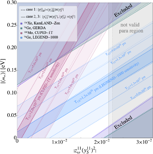
We show the contour with the effective neutrino mass |mee||\langle m_{ee}\rangle| in the unit of eV{\rm{eV}} and the couplings |zω11(yS11)2||z_{\omega}^{11}(y_{S}^{11})^{2}| in Fig. 4 and Fig. 5. The purple and green regions (upper and lower corners) are excluded by the 0νββ0\nu\beta\beta decay experiments KamLAND-Zen [9] and GERDA [10]. The red and blue regions correspond to the survival areas for the experiments CUPID-1T [11] and LEGEND-1000 [12] if we assume that no signals are found and set the half-lifetime to T1/2>5.0×1025T_{1/2}>5.0\times 10^{25} yrs (CUPID) and 5.0×10265.0\times 10^{26} yrs (LEGEND), whereas the inner darker areas relate to the sensitivities. We show all the three cases in Fig. 4, with the assumption |y1SL11|=|y1SR11||y_{1SL}^{\prime 11}|=|y_{1SR}^{11}| for case 1. Under this assumption, the term that contains ϵ1,2RRL\epsilon_{1,2}^{RRL} and ϵν\epsilon_{\nu} dominants in the inverse half-life expression. Due to the cancellation between the standard light neutrino exchange contribution and the new physics contribution, the 0νββ0\nu\beta\beta decay could be hidden when the relations are linear or almost linear,

(yS11)2zω11300×νβ1β2/4meeeV×(1.5TeVμ)(MS1.5TeV)4(Mω8TeV)2,\displaystyle(y_{S}^{*11})^{2}z_{\omega}^{11}\simeq 300\times\dfrac{\mathcal{M}_{\nu}}{\beta_{1}-\beta_{2}/4}\dfrac{\langle m_{ee}\rangle}{\rm{eV}}\times\left(\dfrac{1.5~{}{\rm{TeV}}}{\mu}\right)\left(\dfrac{M_{S}}{1.5~{}{\rm{TeV}}}\right)^{4}\left(\dfrac{M_{\omega}}{8~{}{\rm{TeV}}}\right)^{2}\,, (51)

where the specific value of ν/(β1β2/4)\mathcal{M}_{\nu}/(\beta_{1}-\beta_{2}/4) varies from isotope to isotope. For the current experiments, the relation can be realized successfully due to the similar ratio value of ν/(β1β2/4)\mathcal{M}_{\nu}/(\beta_{1}-\beta_{2}/4) in Ge76{}^{76}{\rm{Ge}} and Xe136{}^{136}{\rm{Xe}} isotopes. Things will be different and intriguing when the next-generation experiments with Mo100{}^{100}{\rm{Mo}} isotope, e.g. AMoRE-II [85] and CUPID-1T, push the half-life to be order of 1026yrs10^{26}~{}{\rm{yrs}}. The slope of the band with Mo100{}^{100}{\rm{Mo}} is different from Ge76{}^{76}{\rm{Ge}} or Xe136{}^{136}{\rm{Xe}}, leading to the overlap of survival areas being narrowed. With the high sensitivity of the future CUPID-1T and LEGEND-1000 experiments, the survival band can be examined comprehensively. If there is no signal of 0νββ0\nu\beta\beta decays, the survival region will be reduced to the overlap area. On the other hand, if we see the signals in one experiment, the corresponding contour lines will be suitable. The other experiment can help us search for the appropriate region of the lines.

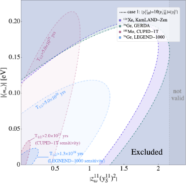
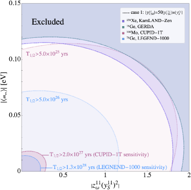
We show the contour of case 1 with assumption |y1SL11||y1SR11||yS11||y_{1SL}^{\prime 11}|\ll|y_{1SR}^{11}|\equiv|y_{S}^{11}| in Fig. 5. This assumption is natural as the allowed regions have ten times difference, and the influence on the neutrino mass is negligible. The survival region is elliptical instead. The left panel refers to |y1SR11|=10|y1SL11||y_{1SR}^{11}|=10|y_{1SL}^{\prime 11}|. One can find that the constraint on the effective Majorana neutrino mass can be larger than the one with only standard neutrino exchange considered |mee|0.2eV|\langle m_{ee}\rangle|\lesssim 0.2~{}{\rm{eV}}. The experiment with Mo100{}^{100}{\rm{Mo}} isotopes can help to reduce the survival area which is similar to what we discussed before. The right panel refers to |y1SR11|=50|y1SL11||y_{1SR}^{11}|=50|y_{1SL}^{\prime 11}| and the effect of the combined analysis with different experiments is not apparent. The bound on the couplings given by experiments KamLAND-Zen and GERDA are

|zω11(yS11)2|<1.8×(1.5TeVμ)(MS1.5TeV)4(Mω8TeV)2.\displaystyle|z_{\omega}^{11}(y_{S}^{11})^{2}|<1.8\times\left(\dfrac{1.5~{}{\text{TeV}}}{\mu}\right)\left(\dfrac{M_{S}}{1.5~{}\text{TeV}}\right)^{4}\left(\dfrac{M_{\omega}}{8~{}\text{TeV}}\right)^{2}\,. (52)

The limits will be more stringent in next generation 0νββ0\nu\beta\beta decay experiments, which have the potential to restrict |zω11(yS11)2||z_{\omega}^{11}(y_{S}^{11})^{2}| at 𝒪(101)\mathcal{O}({10^{-1}}) scale.

IV Summary

In this paper, we have discussed the neutrinoless double beta decay in the colored Zee-Babu model. We study all three cases for the colored Zee-Babu model with a leptoquark and a diquark. The tiny neutrino masses are generated at two-loop level, and neutrinoless double beta decay gets additional contribution from the leptoquarks. We set some texture zeros for the Yukawa coupling matrices to evade constraints from various lepton flavor violation processes. We obtain the allowed regions of parameters after considering the constraints given by tree-level flavor violation processed and charged lepton anomalous magnetic moment.

We have discussed the short-range and standard neutrino exchange mechanisms of neutrinoless double beta decay for each case. The short-range contribution can be realized at tree-level. The general formula of the short-range contributions via the effective field theory approach is briefly reviewed. We adopt the values of nuclear matrix elements calculated with the microscopic interacting boson model and consider the leading order QCD running correction. We give numerical analysis for the three cases with the current experimental results and sensitivities of next-generation experiments. We find that the neutrinoless double beta decay can be hidden with a linear relation in all the cases under certain conditions. The relation can be examined by future 0νββ0\nu\beta\beta decay experiments. The complementary analysis of the different isotope experiments can help reduce the overlap area of the survival region.

Acknowledgements. This work is supported in part by the National Science Foundation of China (12175082, 11775093).

References

  • Cheng and Li [1980] T. P. Cheng and L.-F. Li, Phys. Rev. D 22, 2860 (1980).
  • Petcov and Toshev [1984] S. T. Petcov and S. T. Toshev, Phys. Lett. B 143, 175 (1984).
  • Zee [1986] A. Zee, Nucl. Phys. B 264, 99 (1986).
  • Babu [1988] K. S. Babu, Phys. Lett. B 203, 132 (1988).
  • Babu and Julio [2010] K. S. Babu and J. Julio, Nucl. Phys. B 841, 130 (2010), eprint 1006.1092.
  • Angel et al. [2013] P. W. Angel, Y. Cai, N. L. Rodd, M. A. Schmidt, and R. R. Volkas, JHEP 10, 118 (2013), [Erratum: JHEP 11, 092 (2014)], eprint 1308.0463.
  • Aristizabal Sierra et al. [2015] D. Aristizabal Sierra, A. Degee, L. Dorame, and M. Hirsch, JHEP 03, 040 (2015), eprint 1411.7038.
  • Cao et al. [2018] Q.-H. Cao, S.-L. Chen, E. Ma, B. Yan, and D.-M. Zhang, Phys. Lett. B 779, 430 (2018), eprint 1707.05896.
  • Gando et al. [2016] A. Gando et al. (KamLAND-Zen), Phys. Rev. Lett. 117, 082503 (2016), [Addendum: Phys.Rev.Lett. 117, 109903 (2016)], eprint 1605.02889.
  • Agostini et al. [2020] M. Agostini et al. (GERDA), Phys. Rev. Lett. 125, 252502 (2020), eprint 2009.06079.
  • Armatol et al. [2022] A. Armatol et al. (CUPID) (2022), eprint 2203.08386.
  • Abgrall et al. [2021] N. Abgrall et al. (LEGEND) (2021), eprint 2107.11462.
  • Prezeau et al. [2003] G. Prezeau, M. Ramsey-Musolf, and P. Vogel, Phys. Rev. D 68, 034016 (2003), eprint hep-ph/0303205.
  • del Aguila et al. [2012] F. del Aguila, A. Aparici, S. Bhattacharya, A. Santamaria, and J. Wudka, JHEP 06, 146 (2012), eprint 1204.5986.
  • Cirigliano et al. [2017] V. Cirigliano, W. Dekens, J. de Vries, M. L. Graesser, and E. Mereghetti, JHEP 12, 082 (2017), eprint 1708.09390.
  • Deppisch et al. [2018] F. F. Deppisch, L. Graf, J. Harz, and W.-C. Huang, Phys. Rev. D 98, 055029 (2018), eprint 1711.10432.
  • Cirigliano et al. [2018] V. Cirigliano, W. Dekens, J. de Vries, M. L. Graesser, and E. Mereghetti, JHEP 12, 097 (2018), eprint 1806.02780.
  • Gráf et al. [2022] L. Gráf, M. Lindner, and O. Scholer (2022), eprint 2204.10845.
  • Pas et al. [1998] H. Pas, M. Hirsch, S. G. Kovalenko, and H. V. Klapdor-Kleingrothaus, Prog. Part. Nucl. Phys. 40, 283 (1998), eprint hep-ph/9712361.
  • Pas et al. [1999] H. Pas, M. Hirsch, H. V. Klapdor-Kleingrothaus, and S. G. Kovalenko, Phys. Lett. B 453, 194 (1999).
  • Helo et al. [2016] J. C. Helo, M. Hirsch, and T. Ota, JHEP 06, 006 (2016), eprint 1602.03362.
  • Kotila et al. [2021] J. Kotila, J. Ferretti, and F. Iachello (2021), eprint 2110.09141.
  • Pas et al. [2001] H. Pas, M. Hirsch, H. V. Klapdor-Kleingrothaus, and S. G. Kovalenko, Phys. Lett. B 498, 35 (2001), eprint hep-ph/0008182.
  • Graf et al. [2018] L. Graf, F. F. Deppisch, F. Iachello, and J. Kotila, Phys. Rev. D 98, 095023 (2018), eprint 1806.06058.
  • Bonnet et al. [2013] F. Bonnet, M. Hirsch, T. Ota, and W. Winter, JHEP 03, 055 (2013), [Erratum: JHEP 04, 090 (2014)], eprint 1212.3045.
  • Chen et al. [2021] P.-T. Chen, G.-J. Ding, and C.-Y. Yao, JHEP 12, 169 (2021), eprint 2110.15347.
  • Helo et al. [2013] J. C. Helo, M. Hirsch, H. Päs, and S. G. Kovalenko, Phys. Rev. D 88, 073011 (2013), eprint 1307.4849.
  • Deppisch et al. [2020] F. F. Deppisch, L. Graf, F. Iachello, and J. Kotila, Phys. Rev. D 102, 095016 (2020), eprint 2009.10119.
  • Kohda et al. [2013] M. Kohda, H. Sugiyama, and K. Tsumura, Phys. Lett. B 718, 1436 (2013), eprint 1210.5622.
  • Nomura and Okada [2016] T. Nomura and H. Okada, Phys. Rev. D 94, 075021 (2016), eprint 1607.04952.
  • Chang et al. [2016] W.-F. Chang, S.-C. Liou, C.-F. Wong, and F. Xu, JHEP 10, 106 (2016), eprint 1608.05511.
  • Guo et al. [2018] S.-Y. Guo, Z.-L. Han, B. Li, Y. Liao, and X.-D. Ma, Nucl. Phys. B 928, 435 (2018), eprint 1707.00522.
  • Ding et al. [2018] R. Ding, Z.-L. Han, L. Huang, and Y. Liao, Chin. Phys. C 42, 103101 (2018), eprint 1802.05248.
  • Datta et al. [2019] A. Datta, D. Sachdeva, and J. Waite, Phys. Rev. D 100, 055015 (2019), eprint 1905.04046.
  • Saad [2020] S. Saad, Phys. Rev. D 102, 015019 (2020), eprint 2005.04352.
  • Babu et al. [2021] K. S. Babu, P. S. B. Dev, S. Jana, and A. Thapa, JHEP 03, 179 (2021), eprint 2009.01771.
  • Hirsch et al. [1996a] M. Hirsch, H. V. Klapdor-Kleingrothaus, and S. G. Kovalenko, Phys. Lett. B 378, 17 (1996a), eprint hep-ph/9602305.
  • Hirsch et al. [1996b] M. Hirsch, H. V. Klapdor-Kleingrothaus, and S. G. Kovalenko, Phys. Rev. D 54, R4207 (1996b), eprint hep-ph/9603213.
  • Davies and He [1991] A. J. Davies and X.-G. He, Phys. Rev. D 43, 225 (1991).
  • Doršner et al. [2016] I. Doršner, S. Fajfer, A. Greljo, J. F. Kamenik, and N. Košnik, Phys. Rept. 641, 1 (2016), eprint 1603.04993.
  • Sirunyan et al. [2019a] A. M. Sirunyan et al. (CMS), Phys. Rev. D 99, 052002 (2019a), eprint 1811.01197.
  • Aad et al. [2020] G. Aad et al. (ATLAS), JHEP 10, 112 (2020), eprint 2006.05872.
  • Aaboud et al. [2019] M. Aaboud et al. (ATLAS), Eur. Phys. J. C 79, 733 (2019), eprint 1902.00377.
  • Sirunyan et al. [2019b] A. M. Sirunyan et al. (CMS), Phys. Rev. D 99, 032014 (2019b), eprint 1808.05082.
  • Sirunyan et al. [2018] A. M. Sirunyan et al. (CMS), Eur. Phys. J. C 78, 707 (2018), eprint 1803.02864.
  • Chatrchyan et al. [2012] S. Chatrchyan et al. (CMS), JHEP 12, 055 (2012), eprint 1210.5627.
  • Sirunyan et al. [2020] A. M. Sirunyan et al. (CMS), JHEP 05, 033 (2020), eprint 1911.03947.
  • Babu and Macesanu [2003] K. S. Babu and C. Macesanu, Phys. Rev. D 67, 073010 (2003), eprint hep-ph/0212058.
  • Abe et al. [2021] K. Abe et al. (Super-Kamiokande), Phys. Rev. D 103, 012008 (2021), eprint 2012.02607.
  • Chang and Chang [1980] L. N. Chang and N. P. Chang, Phys. Lett. B 92, 103 (1980).
  • Kuo and Love [1980] T.-K. Kuo and S. T. Love, Phys. Rev. Lett. 45, 93 (1980).
  • Rao and Shrock [1982] S. Rao and R. Shrock, Phys. Lett. B 116, 238 (1982).
  • Rao and Shrock [1984] S. Rao and R. E. Shrock, Nucl. Phys. B 232, 143 (1984).
  • Caswell et al. [1983] W. E. Caswell, J. Milutinovic, and G. Senjanovic, Phys. Lett. B 122, 373 (1983).
  • Buchoff and Wagman [2016] M. I. Buchoff and M. Wagman, Phys. Rev. D 93, 016005 (2016), [Erratum: Phys.Rev.D 98, 079901 (2018)], eprint 1506.00647.
  • Rinaldi et al. [2019] E. Rinaldi, S. Syritsyn, M. L. Wagman, M. I. Buchoff, C. Schroeder, and J. Wasem, Phys. Rev. D 99, 074510 (2019), eprint 1901.07519.
  • Oosterhof et al. [2019] F. Oosterhof, B. Long, J. de Vries, R. G. E. Timmermans, and U. van Kolck, Phys. Rev. Lett. 122, 172501 (2019), eprint 1902.05342.
  • Fridell et al. [2021] K. Fridell, J. Harz, and C. Hati, JHEP 11, 185 (2021), eprint 2105.06487.
  • Takenaka et al. [2020] A. Takenaka et al. (Super-Kamiokande), Phys. Rev. D 102, 112011 (2020), eprint 2010.16098.
  • Aoki et al. [2017] Y. Aoki, T. Izubuchi, E. Shintani, and A. Soni, Phys. Rev. D 96, 014506 (2017), eprint 1705.01338.
  • Yoo et al. [2022] J.-S. Yoo, Y. Aoki, P. Boyle, T. Izubuchi, A. Soni, and S. Syritsyn, Phys. Rev. D 105, 074501 (2022), eprint 2111.01608.
  • Capozzi et al. [2018] F. Capozzi, E. Lisi, A. Marrone, and A. Palazzo, Prog. Part. Nucl. Phys. 102, 48 (2018), eprint 1804.09678.
  • Esteban et al. [2020] I. Esteban, M. C. Gonzalez-Garcia, M. Maltoni, T. Schwetz, and A. Zhou, JHEP 09, 178 (2020), eprint 2007.14792.
  • de Salas et al. [2018] P. F. de Salas, D. V. Forero, C. A. Ternes, M. Tortola, and J. W. F. Valle, Phys. Lett. B 782, 633 (2018), eprint 1708.01186.
  • de Salas et al. [2021] P. F. de Salas, D. V. Forero, S. Gariazzo, P. Martínez-Miravé, O. Mena, C. A. Ternes, M. Tórtola, and J. W. F. Valle, JHEP 02, 071 (2021), eprint 2006.11237.
  • Davidson et al. [1994] S. Davidson, D. C. Bailey, and B. A. Campbell, Z. Phys. C 61, 613 (1994), eprint hep-ph/9309310.
  • Leurer [1994a] M. Leurer, Phys. Rev. D 49, 333 (1994a), eprint hep-ph/9309266.
  • Leurer [1994b] M. Leurer, Phys. Rev. D 50, 536 (1994b), eprint hep-ph/9312341.
  • Carpentier and Davidson [2010] M. Carpentier and S. Davidson, Eur. Phys. J. C 70, 1071 (2010), eprint 1008.0280.
  • Bona et al. [2008] M. Bona et al. (UTfit), JHEP 03, 049 (2008), eprint 0707.0636.
  • Abi et al. [2021] B. Abi et al. (Muon g-2), Phys. Rev. Lett. 126, 141801 (2021), eprint 2104.03281.
  • Queiroz and Shepherd [2014] F. S. Queiroz and W. Shepherd, Phys. Rev. D 89, 095024 (2014), eprint 1403.2309.
  • Kotila and Iachello [2012] J. Kotila and F. Iachello, Phys. Rev. C 85, 034316 (2012), eprint 1209.5722.
  • Azzolini et al. [2018] O. Azzolini et al. (CUPID-0), Phys. Rev. Lett. 120, 232502 (2018), eprint 1802.07791.
  • Armengaud et al. [2021] E. Armengaud et al. (CUPID), Phys. Rev. Lett. 126, 181802 (2021), eprint 2011.13243.
  • Arnaboldi et al. [2003] C. Arnaboldi et al., Phys. Lett. B 557, 167 (2003), eprint hep-ex/0211071.
  • Adams et al. [2021] D. Q. Adams et al. (CUORE) (2021), eprint 2104.06906.
  • Helo et al. [2015] J. C. Helo, M. Hirsch, T. Ota, and F. A. Pereira dos Santos, JHEP 05, 092 (2015), eprint 1502.05188.
  • Mahajan [2014] N. Mahajan, Phys. Rev. Lett. 112, 031804 (2014), eprint 1310.1064.
  • González et al. [2016] M. González, M. Hirsch, and S. G. Kovalenko, Phys. Rev. D 93, 013017 (2016), [Erratum: Phys.Rev.D 97, 099907 (2018)], eprint 1511.03945.
  • Arbeláez et al. [2016] C. Arbeláez, M. González, M. Hirsch, and S. Kovalenko, Phys. Rev. D 94, 096014 (2016), [Erratum: Phys.Rev.D 97, 099904 (2018)], eprint 1610.04096.
  • Arbeláez et al. [2017] C. Arbeláez, M. González, S. Kovalenko, and M. Hirsch, Phys. Rev. D 96, 015010 (2017), eprint 1611.06095.
  • González et al. [2018] M. González, M. Hirsch, and S. Kovalenko, Phys. Rev. D 97, 115005 (2018), eprint 1711.08311.
  • Ayala et al. [2020] C. Ayala, G. Cvetic, and L. Gonzalez, Phys. Rev. D 101, 094003 (2020), eprint 2001.04000.
  • Lee [2020] M. H. Lee (AMoRE), JINST 15, C08010 (2020), eprint 2005.05567.