The neutrino force in neutrino backgrounds: Spin dependence and parity-violating effects

When both propagators in Eq. (12) take the vacuum part, the integral gives the vacuum contribution to the neutrino force:

	$\displaystyle I_{0}^{\mu\nu}$	$\displaystyle=-\frac{{\rm i}}{8}\int\frac{{\rm d}^{4}k}{\left(2\pi\right)^{4}}\frac{{\rm Tr}\left[\gamma^{\mu}\left(1-\gamma_{5}\right)\left(\not{k}+\not{q}\right)\gamma^{\nu}\left(1-\gamma_{5}\right)\not{k}\right]}{k^{2}\left(k+q\right)^{2}}$
		$\displaystyle=-\frac{1}{144\pi^{2}}\left[5+3\Delta_{\rm E}+3\log\left(\frac{\mu^{2}}{-q^{2}}\right)\right]\left(q^{\mu}q^{\nu}-q^{2}g^{\mu\nu}\right)\;,$		(15)

where we have neglected the tiny neutrino mass for simplicity, $\mu$ is the renormalization scale and $\Delta_{\rm E}\equiv 1/\epsilon-\gamma_{\rm E}+\log\left(4\pi\right)$ with $\gamma_{\rm E}\approx 0.557$ the Euler-Mascheroni constant. (For the complete expression of the parity-violating neutrino force in vacuum, which includes finite neutrino masses and lepton flavor mixing, see Ref. Ghosh:2019dmi ). The term proportional to $g^{00}$ in Eq. (2.1) leads to the spin-independent potential of the neutrino force:

$\displaystyle V_{0}^{\rm SI}(r)=g_{V}^{\chi_{1}}g_{V}^{\chi_{2}}V_{0}(r)\;,$

(16)

with $V_{0}(r)$ given by Eq. (2). Note that the terms depending on $\mu$ and $1/\epsilon$ vanish after taking the Fourier transform since they do not have a branch cut on the complex plane of $q$. The $g^{ii},(i=1,2,3)$ and $q^{\mu}q^{\nu}$ terms in Eq. (2.1), using the results of Fourier transform in Appendix A, give rise to a spin-dependent parity-conserving (SD-PC) contribution to the potential:

$\displaystyle V_{0}^{\text{SD-PC}}({\bf r})=\frac{1}{2}g_{A}^{\chi_{1}}g_{A}^{\chi_{2}}\left[5\left(\boldsymbol{\sigma}_{1}\cdot\bf{\hat{r}}\right)\left(\boldsymbol{\sigma}_{2}\cdot\bf{\hat{r}}\right)-3\left(\boldsymbol{\sigma}_{1}\cdot\boldsymbol{\sigma}_{2}\right)\right]V_{0}(r)\;,$

(17)

with ${\bf\hat{r}}\equiv{\bf r}/r$. Note that in Eq. (17) $\boldsymbol{\sigma}_{1}$ and $\boldsymbol{\sigma}_{2}$ are axial vectors and ${\bf\hat{r}}$ is a vector. Each term contains an even number of axial vectors, implying that the potential is invariant under parity transformation.

Here, we would like to clarify the connection between spin dependence and parity violation. A force being spin-dependent does not necessarily mean that it is parity-violating, but a parity-violating force is always spin-dependent. The latter is labeled as SD-PV throughout this work.

In the vacuum case, the SD-PV part of the force comes from the sub-leading term in $v$ of the contraction between $W_{\mu\nu}$ and the $g^{\mu\nu}$ term in Eq. (2.1). This part has been calculated in Ref. Ghosh:2019dmi ,

	$\displaystyle V_{0}^{\text{SD-PV}}({\bf r})=$	$\displaystyle\left[H_{11}\left(\boldsymbol{\sigma}_{1}\cdot\boldsymbol{v}_{1}\right)+H_{12}\left(\boldsymbol{\sigma}_{1}\cdot\boldsymbol{v}_{2}\right)+H_{21}\left(\boldsymbol{\sigma}_{2}\cdot\boldsymbol{v}_{1}\right)+H_{22}\left(\boldsymbol{\sigma}_{2}\cdot\boldsymbol{v}_{2}\right)\right.$
		$\displaystyle\left.+C\left(\boldsymbol{\sigma}_{1}\times\boldsymbol{\sigma}_{2}\right)\cdot\nabla\right]V_{0}(r)\;,$		(18)

where

$\displaystyle H_{11}=-H_{12}=2g_{V}^{\chi_{2}}g_{A}^{\chi_{1}}\;,\quad H_{22}=-H_{21}=2g_{V}^{\chi_{1}}g_{A}^{\chi_{2}}\;,\quad C=\frac{g_{V}^{\chi_{1}}g_{A}^{\chi_{2}}}{m_{1}}+\frac{g_{V}^{\chi_{2}}g_{A}^{\chi_{1}}}{m_{2}}\;.$

(19)

Compared to Eq. (17), Eq. (2.1) is suppressed by either the velocities of external particles, $\left|\boldsymbol{v}_{i}\right|$ (for $i=1,2$), or by the variation of the velocities

$\displaystyle\frac{\nabla}{m_{i}}\sim\frac{{\bf q}}{m_{i}}\sim\left|\boldsymbol{v}_{i}^{\prime}-\boldsymbol{v}_{i}\right|\;,$

(20)

where $\boldsymbol{v}_{i}$ and $\boldsymbol{v}_{i}^{\prime}$ denote the incident and outgoing velocity of $\chi_{i}$, respectively. Throughout this paper, we refer to the suppression in either way as the velocity suppression.

The total neutrino force in vacuum is then obtained by adding Eqs. (16)-(2.1) together:

$\displaystyle V_{0}\left({\bf r}\right)=V_{0}^{{\rm SI}}(r)+V_{0}^{\text{SD-PC}}({\bf r})+V_{0}^{\text{SD-PV}}({\bf r})\;.$

(21)

The first two terms are of order ${\cal O}(v^{0})$, the third term is of order ${\cal O}(v)$, and we have neglected higher-ordered terms ${\cal O}(v^{2})$. There are no first-order corrections to the first two terms, because any term proportional to ${\cal O}(v)$ violates parity and belongs to the third term, see Eqs. (130)-(133).

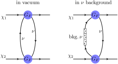
We turn to the study of background corrections to the spin-dependent neutrino force. First, we note that there is no effect from the term when both propagators take the background part. The result is proportional to the product of two $\delta$-functions which have different arguments, and it vanishes. This can be understood as follows: If both neutrinos in Fig. 2 are on-shell, then both of them come from the background. As a result, there is no neutrino exchanged between $\chi_{1}$ and $\chi_{2}$, and therefore, there is no force between them.

The background term comes from the cross terms in Eq. (12), i.e., one propagator takes the vacuum part, and the other takes the background part (see the right panel of Fig. 2). We find that, in general, the background integral can be decomposed into two parts,

$\displaystyle I_{\rm bkg}^{\mu\nu}\left({\bf q}\right)=I_{\rm PC}^{\mu\nu}\left({\bf q}\right)+I_{\rm PV}^{\mu\nu}\left({\bf q}\right)\;,$

(22)

where

$\displaystyle I_{\rm PC}^{\mu\nu}\left({\bf q}\right)=-\int{\rm d}\widetilde{\bf k}\int{\rm d}\widetilde{k}^{0}\left\{\frac{2k^{\mu}k^{\nu}+k^{\mu}q^{\nu}+k^{\nu}q^{\mu}-g^{\mu\nu}\left(m_{\nu}^{2}-{\bf k}\cdot{\bf q}\right)}{2{\bf k}\cdot{\bf q}+{\bf q}^{2}}+\left(q\to-q\right)\right\}\;,$

(23)

and

$\displaystyle I_{\rm PV}^{\mu\nu}\left({\bf q}\right)={\rm i}\epsilon^{\mu\nu\rho\sigma}q_{\sigma}\int{\rm d}\widetilde{\bf k}\int{\rm d}\widetilde{k}^{0}\left[\frac{k_{\rho}}{2{\bf k}\cdot{\bf q}+{\bf q}^{2}}+\left(q\to-q\right)\right]\;.$

(24)

Here $\epsilon^{\mu\nu\rho\sigma}$ is the Levi-Civita tensor, and we have used the following notations:

	$\displaystyle\int{\rm d}\widetilde{\bf k}$	$\displaystyle\equiv\int\frac{{\rm d}^{3}{\bf k}}{\left(2\pi\right)^{3}}\frac{1}{2E_{\bf k}}\;,$
	$\displaystyle\int{\rm d}\widetilde{k}^{0}$	$\displaystyle\equiv\int_{-\infty}^{\infty}{\rm d}k^{0}\left[\delta\left(k^{0}-E_{\bf k}\right)\Theta\left(k^{0}\right)n_{+}({\bf k})+\delta\left(k^{0}+E_{\bf k}\right)\Theta\left(-k^{0}\right)n_{-}({\bf k})\right]\;,$		(25)

with $E_{\bf k}\equiv\sqrt{{\bf k}^{2}+m_{\nu}^{2}}$. Due to the effective violation of Lorentz invariance by the neutrino background, the term proportional to $\epsilon^{\mu\nu\rho\sigma}$ is no longer vanishing as in the vacuum scenario. In fact, one can verify that (see Appendix B for more details)

$\displaystyle I_{\rm PC}^{\mu\nu}\left(-{\bf q}\right)=I_{\rm PC}^{\mu\nu}\left({\bf q}\right)\;,\quad I_{\rm PV}^{\mu\nu}\left(-{\bf q}\right)=-I_{\rm PV}^{\mu\nu}\left({\bf q}\right)\;.$

(26)

In vacuum, the parity-violating neutrino force only comes from the wave-function part in Eq. (8). Technically, this is due to the fact that the vacuum loop integral in Eq. (2.1) is invariant under the momentum reflection, i.e., $I_{0}^{\mu\nu}(-{\bf q})=I_{0}^{\mu\nu}({\bf q})$. However, unlike in the vacuum case, the loop integral (24) in the background is not invariant under the momentum reflection. This leads to additional contributions to the parity-violating neutrino force, as shown below. Similarly, we can also decompose the wave functions (8) into two parts,

$\displaystyle W_{\mu\nu}\left({\bf p}_{i}\right)=W_{\mu\nu}^{\rm PC}\left({\bf p}_{i}\right)+W_{\mu\nu}^{\rm PV}\left({\bf p}_{i}\right)\;.$

(27)

For the specific forms of $W_{\mu\nu}^{\rm PC}$ and $W_{\mu\nu}^{\rm PV}$, we refer to Appendix B. Under reflection of the external momentum ${\bf p}_{i}\to-{\bf p}_{i}$, the first term is invariant while the second term changes sign

$\displaystyle W^{\rm PC}_{\mu\nu}\left(-{\bf p}_{i}\right)=W^{\rm PC}_{\mu\nu}\left({\bf p}_{i}\right)\;,\quad W^{\rm PV}_{\mu\nu}\left(-{\bf p}_{i}\right)=-W^{\rm PV}_{\mu\nu}\left({\bf p}_{i}\right)\;.$

(28)

We note that $W^{\rm PV}_{\mu\nu}$ is suppressed by the velocities of the external particles compared with $W^{\rm PC}_{\mu\nu}$. This is the reason the parity-violating neutrino force in vacuum, Eq. (2.1), is velocity suppressed, since in vacuum the only source of parity violation comes from $W_{\mu\nu}^{\rm PV}$.

The components of $I_{\rm bkg}^{\mu\nu}$ and $W_{\mu\nu}$ have been explicitly computed in Appendix B. The $(0,0)$ components of $I^{\mu\nu}_{\rm PC}$ and $W_{\mu\nu}^{\rm PC}$ give the spin-independent background amplitude,

$\displaystyle{\cal A}_{\rm bkg}^{\rm SI}({\bf q})=-4G_{F}^{2}I_{\rm PC}^{00}W_{00}^{\rm PC}=8G_{F}^{2}g_{V}^{\chi_{1}}g_{V}^{\chi_{2}}\int{\rm d}\widetilde{\bf k}\left[n_{+}({\bf k})+n_{-}({\bf k})\right]K_{0}\;,$

(29)

where

$\displaystyle K_{0}=\frac{\left(2{\bf k}^{2}+m_{\nu}^{2}\right){\bf q}^{2}-2\left({\bf k}\cdot{\bf q}\right)^{2}}{{\bf q}^{4}-4\left({\bf k}\cdot{\bf q}\right)^{2}}\;.$

(30)

The amplitude in Eq. (29) is parity conserving and has been analyzed in Ref. Ghosh:2022nzo . The parity-conserving and spin-dependent background amplitude is given, to leading order in the velocity of external particles, by

	$\displaystyle{\cal A}_{{\rm bkg}}^{\text{SD-PC}}({\bf q})=$	$\displaystyle-4G_{F}^{2}\left(I_{{\rm PC}}^{ij}W_{ij}^{{\rm PC}}+I_{{\rm PC}}^{0i}W_{0i}^{{\rm PC}}+I_{{\rm PC}}^{i0}W_{i0}^{{\rm PC}}\right)$
	$\displaystyle=$	$\displaystyle+8G_{F}^{2}g_{A}^{\chi_{1}}g_{A}^{\chi_{2}}\boldsymbol{\sigma}_{1}^{i}\boldsymbol{\sigma}_{2}^{j}\int{\rm d}\widetilde{{\bf k}}\left[n_{+}({\bf k})+n_{-}({\bf k})\right]K_{+}^{ij}$
		$\displaystyle-16G_{F}^{2}\left(g_{V}^{\chi_{1}}g_{A}^{\chi_{2}}\boldsymbol{\sigma}_{2}^{i}+g_{V}^{\chi_{2}}g_{A}^{\chi_{1}}\boldsymbol{\sigma}_{1}^{i}\right)\int{\rm d}\widetilde{{\bf k}}\left[n_{+}({\bf k})-n_{-}({\bf k})\right]K_{-}^{i}\;,$		(31)

where

	$\displaystyle K_{+}^{ij}$	$\displaystyle=\frac{2k^{i}k^{j}{\bf q}^{2}-2\left(k^{i}q^{j}+k^{j}q^{i}\right)\left({\bf k}\cdot{\bf q}\right)+\delta^{ij}\left[2\left({\bf k}\cdot{\bf q}\right)^{2}+m_{\nu}^{2}{\bf q}^{2}\right]}{{\bf q}^{4}-4\left({\bf k}\cdot{\bf q}\right)^{2}}\;,$		(32)
	$\displaystyle K_{-}^{i}$	$\displaystyle=E_{{\bf k}}\frac{k^{i}{\bf q}^{2}-q^{i}\left({\bf k}\cdot{\bf q}\right)}{{\bf q}^{4}-4\left({\bf k}\cdot{\bf q}\right)^{2}}\;.$		(33)

Note that the $K_{-}$ term is suppressed by the neutrino-antineutrino asymmetry of the background, and it vanishes when the background is isotropic.

The parity-violating background amplitude turns out to be

$\displaystyle{\cal A}_{\rm bkg}^{\text{SD-PV}}\left({\bf q}\right)=-4G_{F}^{2}\left(I_{\rm PV}^{\mu\nu}W_{\mu\nu}^{\rm PC}+I_{\rm PC}^{\mu\nu}W_{\mu\nu}^{\rm PV}\right)\;,$

(34)

where the relevant components are given in Eqs. (120)-(133). We can split the parity-violating amplitude into two parts, according to the order of the velocity of external particles:

$\displaystyle{\cal A}_{\rm bkg}^{\text{SD-PV}}\left({\bf q}\right)={\cal A}_{\rm bkg,0}^{\text{SD-PV}}\left({\bf q}\right)+{\cal A}_{\rm bkg,1}^{\text{SD-PV}}\left({\bf q}\right)\;.$

(35)

The first term in Eq. (35) does not depend on the velocity:

	$\displaystyle{\cal A}_{\rm bkg,0}^{\text{SD-PV}}\left({\bf q}\right)=$	$\displaystyle-4G_{F}^{2}I_{\rm PV}^{\mu\nu}W_{\mu\nu}^{\rm PC}$
	$\displaystyle=$	$\displaystyle+8{\rm i}\,G_{F}^{2}g_{A}^{\chi_{1}}g_{A}^{\chi_{2}}\epsilon^{ijk}\boldsymbol{\sigma}_{1}^{i}\boldsymbol{\sigma}_{2}^{j}\int{\rm d}\widetilde{\bf k}\left[n_{+}({\bf k})-n_{-}({\bf k})\right]E_{\bf k}\frac{q^{k}{\bf q}^{2}}{{\bf q}^{4}-4\left({\bf k}\cdot{\bf q}\right)^{2}}$
		$\displaystyle+8{\rm i}\,G_{F}^{2}\left(g_{V}^{\chi_{1}}g_{A}^{\chi_{2}}\boldsymbol{\sigma}_{2}-g_{V}^{\chi_{2}}g_{A}^{\chi_{1}}\boldsymbol{\sigma}_{1}\right)^{i}\int{\rm d}\widetilde{\bf k}\left[n_{+}({\bf k})+n_{-}({\bf k})\right]\frac{\epsilon^{ijk}k^{j}q^{k}{\bf q}^{2}}{{\bf q}^{4}-4\left({\bf k}\cdot{\bf q}\right)^{2}}\;.$		(36)

We note that for neutrino-antineutrino symmetric distributions ($n_{+}=n_{-}$), the first term of Eq. (2.2) vanishes, while the second term proportional to $(n_{+}+n_{-})$ vanishes if $n_{\pm}$ are invariant under ${\bf k}\to-{\bf k}$.

The second term in Eq. (35) is velocity suppressed:

	$\displaystyle{\cal A}_{{\rm bkg},1}^{\text{SD-PV}}\left({\bf q}\right)=$	$\displaystyle-4G_{F}^{2}I_{{\rm PC}}^{\mu\nu}W_{\mu\nu}^{{\rm PV}}$
	$\displaystyle=$	$\displaystyle+16G_{F}^{2}\int{\rm d}\widetilde{{\bf k}}\left[n_{+}({\bf k})+n_{-}({\bf k})\right]\left[g_{V}^{\chi_{2}}g_{A}^{\chi_{1}}\left(\boldsymbol{\sigma}_{1}^{i}\boldsymbol{v}_{1}^{i}K_{0}+\boldsymbol{\sigma}_{1}^{i}\tilde{\boldsymbol{v}}_{2}^{j}K_{+}^{ij}\right)+1\leftrightarrow 2\right]$
		$\displaystyle-32G_{F}^{2}\int{\rm d}\widetilde{{\bf k}}\left[n_{+}({\bf k})-n_{-}({\bf k})\right]K_{-}^{i}\left[g_{V}^{\chi_{1}}g_{V}^{\chi_{2}}\tilde{\boldsymbol{v}}_{1}^{i}+g_{A}^{\chi_{1}}g_{A}^{\chi_{2}}\left(\boldsymbol{\sigma}_{1}\cdot\boldsymbol{v}_{1}\right)\boldsymbol{\sigma}_{2}^{i}+1\leftrightarrow 2\right]\;,$		(37)

where $1\leftrightarrow 2$ denotes terms that exchange the index 1 and 2 for external particles, the reduced velocities are defined as

$\displaystyle\tilde{\boldsymbol{v}}_{1}\equiv\boldsymbol{v}_{1}+{\rm i}\frac{\boldsymbol{\sigma}_{1}\times{\bf q}}{2m_{1}}\;,\quad\tilde{\boldsymbol{v}}_{2}\equiv\boldsymbol{v}_{2}-{\rm i}\frac{\boldsymbol{\sigma}_{2}\times{\bf q}}{2m_{2}}\;,$

(38)

while $K_{0}$, $K_{+}$ and $K_{-}$ are given in Eqs. (30), (32), and (33), respectively. Note that the first term in Eq. (37) is not suppressed by the neutrino-antineutrino asymmetry, while the second term vanishes for isotropic neutrino backgrounds.

The expressions in Eqs. (29), (31), (2.2), and (37) are the comprehensive formulae we derived for the amplitude of the neutrino force in a general neutrino background. They are the main result of this work. Finally, the complete background neutrino force is given by

	$\displaystyle V_{\rm bkg}\left({\bf r}\right)$	$\displaystyle=V_{\rm bkg}^{\rm SI}\left(r\right)+V_{\rm bkg}^{\rm SD-PC}\left({\bf r}\right)+V_{\rm bkg,0}^{\rm SD-PV}\left({\bf r}\right)+V_{\rm bkg,1}^{\rm SD-PV}\left({\bf r}\right)$
		$\displaystyle=-\int\frac{{\rm d}^{3}{\bf q}}{\left(2\pi\right)^{3}}e^{{\rm i}{\bf q}\cdot{\bf r}}\left[{\cal A}_{\rm bkg}^{\rm SI}\left({\bf q}\right)+{\cal A}_{\rm bkg}^{\text{SD-PC}}\left({\bf q}\right)+{\cal A}_{\rm bkg,0}^{\text{SD-PV}}\left({\bf q}\right)+{\cal A}_{\rm bkg,1}^{\text{SD-PV}}\left({\bf q}\right)\right]\;,$		(39)

where each part of the potential is determined by the Fourier transform of the corresponding amplitude.

In particular, for isotropic backgrounds $n_{\pm}({\bf k})=n_{\pm}(\kappa)$, where $\kappa\equiv\left|{\bf k}\right|$, we can first integrate the angular part and obtain the following compact expressions:

	$\displaystyle V_{\rm bkg}^{\rm SI}\left(r\right)$	$\displaystyle=-\frac{G_{F}^{2}g_{V}^{\chi_{1}}g_{V}^{\chi_{2}}}{4\pi^{3}r^{5}}{\cal J}_{a}\;,$		(40)
	$\displaystyle V_{\rm bkg}^{\text{SD-PC}}\left({\bf r}\right)$	$\displaystyle=-\frac{G_{F}^{2}g_{A}^{\chi_{1}}g_{A}^{\chi_{2}}}{4\pi^{3}r^{5}}\left[\left(\boldsymbol{\sigma}_{1}\cdot\boldsymbol{\sigma}_{2}\right){\cal J}_{b}+\left(\boldsymbol{\sigma}_{1}\cdot{\bf\hat{r}}\right)\left(\boldsymbol{\sigma}_{2}\cdot{\bf\hat{r}}\right){\cal J}_{c}\right]\;,$		(41)
	$\displaystyle V_{\rm bkg,0}^{\text{SD-PV}}\left({\bf r}\right)$	$\displaystyle={\hat{\bf r}}\cdot\left(\boldsymbol{\sigma}_{1}\times\boldsymbol{\sigma}_{2}\right)\frac{G_{F}^{2}g_{A}^{\chi_{1}}g_{A}^{\chi_{2}}}{4\pi^{3}r^{5}}{\cal J}_{d}\;,$		(42)
	$\displaystyle V_{\rm bkg,1}^{\text{SD-PV}}\left({\bf r}\right)$	$\displaystyle=-\frac{G_{F}^{2}g_{V}^{\chi_{2}}g_{A}^{\chi_{1}}}{2\pi^{3}r^{5}}\left[\left(\boldsymbol{\sigma}_{1}\cdot\boldsymbol{v}_{1}\right){\cal J}_{a}+\left(\boldsymbol{\sigma}_{1}\cdot\tilde{\boldsymbol{v}}_{2}\right){\cal J}_{b}+\left(\boldsymbol{\sigma}_{1}\cdot{\bf\hat{r}}\right)\left(\tilde{\boldsymbol{v}}_{2}\cdot{\bf\hat{r}}\right){\cal J}_{c}\right]+1\leftrightarrow 2\;.$		(43)

One should keep in mind that in the reduced velocity $\tilde{\boldsymbol{v}}_{i}$ in Eq. (43), ${\bf q}$ should be replaced by $-{\rm i}\nabla$. The dimensionless ${\cal J}$-factors depend on the specific form of the background and can be computed as follows:

	$\displaystyle{\cal J}_{a}$	$\displaystyle=r\int_{0}^{\infty}{\rm d}\kappa\frac{n_{+}(\kappa)+n_{-}(\kappa)}{\sqrt{\kappa^{2}+m_{\nu}^{2}}}\kappa\left[\left(1+m_{\nu}^{2}r^{2}\right)\sin\left(2\kappa r\right)-2\kappa r\cos\left(2\kappa r\right)\right]\;,$		(44)
	$\displaystyle{\cal J}_{b}$	$\displaystyle=r\int_{0}^{\infty}{\rm d}\kappa\frac{n_{+}(\kappa)+n_{-}(\kappa)}{\sqrt{\kappa^{2}+m_{\nu}^{2}}}\kappa\left\{2\kappa r\cos\left(2\kappa r\right)+\left[\left(2\kappa^{2}+m_{\nu}^{2}\right)r^{2}-1\right]\sin\left(2\kappa r\right)\right\}\;,$		(45)
	$\displaystyle{\cal J}_{c}$	$\displaystyle=2r\int_{0}^{\infty}{\rm d}\kappa\frac{n_{+}(\kappa)+n_{-}(\kappa)}{\sqrt{\kappa^{2}+m_{\nu}^{2}}}\kappa\left[\left(1-\kappa^{2}r^{2}\right)\sin\left(2\kappa r\right)-2\kappa r\cos\left(2\kappa r\right)\right]\;,$		(46)
	$\displaystyle{\cal J}_{d}$	$\displaystyle=2r^{2}\int_{0}^{\infty}{\rm d}\kappa\left[n_{+}(\kappa)-n_{-}(\kappa)\right]\kappa\left[\sin\left(2\kappa r\right)-\kappa r\cos\left(2\kappa r\right)\right]\;.$		(47)

Eqs. (40)-(47) are applicable to any isotropic backgrounds. To derive them, we used the Fourier transforms shown in Appendix A. We provide the calculation details in Appendix C.

In the following two sections, we apply the general formulae derived in this section to studying several specific neutrino backgrounds: the cosmic neutrino background (C$\nu$B), the degenerate neutrino gas, and the directional neutrino beams.

The cosmic neutrino background (C$\nu$B) is ubiquitous in the universe and relatively dense compared to artificial neutrino sources.²²2The comparison is in terms of the number of neutrinos per volume: the C$\nu$B number density for each flavor is $56\nu/{\rm cm}^{3}$+$56\overline{\nu}/{\rm cm}^{3}$ assuming Dirac neutrinos Workman:2022ynf , while the reactor neutrino flux at 1 km from a 2.9 GW nuclear power plant is only $5\times 10^{9}/{\rm cm}^{2}/{\rm s}$ Kopeikin:2012zz , corresponding to $0.17$ antineutrinos in a volume of 1 ${\rm cm}^{3}$. The C$\nu$B is approximately isotropic. Assuming the standard cosmological evolution, it can be approximated by the Fermi-Dirac distribution:

$\displaystyle n_{\pm}\left({\bf k}\right)=\frac{1}{e^{\left(\kappa\mp\mu\right)/T}+1}\;,$

(48)

where $\mu$ and $T$ are the chemical potential and temperature of C$\nu$B, respectively. In the standard cosmology, $T\approx 1.9$ K and $\mu/T\ll 1$. Note that in Eq. (48), $T$ should not be interpreted as a temperature but as a quantity that is rescaled from the temperature of neutrino decoupling in the early universe. Hence for massive neutrinos, Eq. (48) is a non-thermal distribution due to $\kappa/T$ instead of $E_{{\bf k}}/T$ occurring in the exponential.

Under certain conditions (to be discussed later), one can use the Maxwell-Boltzmann distribution to approximate the Fermi-Dirac distribution:

$\displaystyle n_{\pm}\left({\bf k}\right)=\exp\left[\left(\pm\mu-\kappa\right)/T\right]\;.$

(49)

This approximation has been frequently used in cosmological calculations for thermal species due to the simplicity of analytically computing various integrals Gondolo:1990dk . And it is known that using Eq. (49) instead of Eq. (48) typically causes $\sim 10\%$ deviations from the true values—see e.g. Eq. (3.6) in EscuderoAbenza:2020cmq or Tab. III in Luo:2020sho . Therefore, in Secs. 3.1.1-3.1.3, our results are obtained assuming the Maxwell-Boltzmann distribution. The differences caused by using the quantum statistics are discussed in Sec. 3.1.4.

References

• (1) H. Bethe and R. A. Bacher, Rev. Mod. Phys. 8, 201 (1936); D. Iwanenko and A. Sokolow, Z. Physik 102, 119 (1936); G. Gamow and E. Teller, Phys. Rev. 51, 289 (1937).
• (2) G. Feinberg and J. Sucher, Long-Range Forces from Neutrino-Pair Exchange, Phys. Rev. 166 (1968) 1638–1644.
• (3) R. P. Feynman, Feynman Lectures on Gravitation, section 2.3. Addison-Wesley, Reading, MA, 1995.
• (4) G. Feinberg, J. Sucher, and C. K. Au, The Dispersion Theory of Dispersion Forces, Phys. Rept. 180 (1989) 83.
• (5) S. D. H. Hsu and P. Sikivie, Long range forces from two neutrino exchange revisited, Phys. Rev. D 49 (1994) 4951–4953, [hep-ph/9211301].
• (6) J. A. Grifols, E. Masso, and R. Toldra, Majorana neutrinos and long range forces, Phys. Lett. B 389 (1996) 563–565, [hep-ph/9606377].
• (7) M. Lusignoli and S. Petrarca, Remarks on the forces generated by two-neutrino exchange, Eur. Phys. J. C 71 (2011) 1568, [1010.3872].
• (8) Q. Le Thien and D. E. Krause, Spin-Independent Two-Neutrino Exchange Potential with Mixing and CPCP-Violation, Phys. Rev. D 99 (2019), no. 11 116006, [1901.05345].
• (9) A. Segarra and J. Bernabéu, Absolute neutrino mass and the Dirac/Majorana distinction from the weak interaction of aggregate matter, Phys. Rev. D 101 (2020), no. 9 093004, [2001.05900].
• (10) Y. V. Stadnik, Probing Long-Range Neutrino-Mediated Forces with Atomic and Nuclear Spectroscopy, Phys. Rev. Lett. 120 (2018), no. 22 223202, [1711.03700].
• (11) M. Ghosh, Y. Grossman, and W. Tangarife, Probing the two-neutrino exchange force using atomic parity violation, Phys. Rev. D 101 (2020), no. 11 116006, [1912.09444].
• (12) P. D. Bolton, F. F. Deppisch, and C. Hati, Probing new physics with long-range neutrino interactions: an effective field theory approach, JHEP 07 (2020) 013, [2004.08328].
• (13) A. Costantino and S. Fichet, The Neutrino Casimir Force, JHEP 09 (2020) 122, [2003.11032].
• (14) X.-j. Xu and B. Yu, On the short-range behavior of neutrino forces beyond the Standard Model: from 1/r5 to 1/r4, 1/r2, and 1/r, JHEP 02 (2022) 008, [2112.03060].
• (15) V. A. Dzuba, V. V. Flambaum, and P. Munro-Laylim, Long-range parity-nonconserving electron-nucleon interaction, Phys. Rev. A 106 (2022), no. 1 012817, [2205.02569].
• (16) P. Munro-Laylim, V. A. Dzuba, and V. V. Flambaum, Effects of the long-range neutrino-mediated force in atomic phenomena, 2207.07325.
• (17) M. Ghosh, Y. Grossman, W. Tangarife, X.-J. Xu, and B. Yu, Neutrino forces in neutrino backgrounds, JHEP 02 (2023) 092, [2209.07082].
• (18) D. Blas, I. Esteban, M. C. Gonzalez-Garcia, and J. Salvado, On neutrino-mediated potentials in a neutrino background, JHEP 04 (2023) 039, [2212.03889].
• (19) K. Van Tilburg, Wake Forces, 2401.08745.
• (20) E. Fischbach, Long range forces and neutrino mass, Annals Phys. 247 (1996) 213–291, [hep-ph/9603396].
• (21) A. Y. Smirnov and F. Vissani, Long range neutrino forces and the lower bound on neutrino mass, hep-ph/9604443.
• (22) A. Abada, M. B. Gavela, and O. Pene, To rescue a star, Phys. Lett. B 387 (1996) 315–319, [hep-ph/9605423].
• (23) M. Kachelriess, Neutrino selfenergy and pair creation in neutron stars, Phys. Lett. B 426 (1998) 89–94, [hep-ph/9712363].
• (24) K. Kiers and M. H. G. Tytgat, Neutrino ground state in a dense star, Phys. Rev. D 57 (1998) 5970–5981, [hep-ph/9712463].
• (25) A. Abada, O. Pene, and J. Rodriguez-Quintero, Finite size effects on multibody neutrino exchange, Phys. Rev. D 58 (1998) 073001, [hep-ph/9802393].
• (26) J. Arafune and Y. Mimura, Finiteness of multibody neutrino exchange potential energy in neutron stars, Prog. Theor. Phys. 100 (1998) 1083–1088, [hep-ph/9805395].
• (27) N. Orlofsky and Y. Zhang, Neutrino as the dark force, Phys. Rev. D 104 (2021), no. 7 075010, [2106.08339].
• (28) R. Coy, X.-J. Xu, and B. Yu, Neutrino forces and the Sommerfeld enhancement, JHEP 06 (2022) 093, [2203.05455].
• (29) P. Brax, S. Fichet, and G. Pignol, Bounding quantum dark forces, Phys. Rev. D 97 (2018), no. 11 115034, [1710.00850].
• (30) S. Fichet, Quantum forces from dark matter and where to find them, Phys. Rev. Lett. 120 (2018), no. 13 131801, [1705.10331].
• (31) A. Costantino, S. Fichet, and P. Tanedo, Exotic spin-dependent forces from a hidden sector, JHEP 03 (2020) 148, [1910.02972].
• (32) H. Banks and M. Mccullough, Charting the fifth force landscape, Phys. Rev. D 103 (2021), no. 7 075018, [2009.12399].
• (33) P. Brax and S. Fichet, Scalar-mediated quantum forces between macroscopic bodies and interferometry, Phys. Dark Univ. 42 (2023) 101294, [2203.01342].
• (34) M. Bauer and G. Rostagni, Fifth Forces from QCD Axions Scale Differently, Phys. Rev. Lett. 132 (2024), no. 10 101802, [2307.09516].
• (35) S. Barbosa and S. Fichet, Background-Induced Forces from Dark Relics, 2403.13894.
• (36) N. P. Landsman and C. G. van Weert, Real and Imaginary Time Field Theory at Finite Temperature and Density, Phys. Rept. 145 (1987) 141.
• (37) D. Notzold and G. Raffelt, Neutrino Dispersion at Finite Temperature and Density, Nucl. Phys. B 307 (1988) 924–936.
• (38) M. Quiros, Finite temperature field theory and phase transitions, in ICTP Summer School in High-Energy Physics and Cosmology, pp. 187–259, 1, 1999. hep-ph/9901312.
• (39) J. I. Kapusta and C. Gale, Finite-temperature field theory: Principles and applications. Cambridge Monographs on Mathematical Physics. Cambridge University Press, 2011.
• (40) M. Laine and A. Vuorinen, Basics of Thermal Field Theory, vol. 925. Springer, 2016.
• (41) Particle Data Group Collaboration, R. L. Workman and Others, Review of Particle Physics, PTEP 2022 (2022) 083C01.
• (42) V. I. Kopeikin, Flux and spectrum of reactor antineutrinos, Phys. Atom. Nucl. 75 (2012) 143–152.
• (43) P. Gondolo and G. Gelmini, Cosmic abundances of stable particles: Improved analysis, Nucl. Phys. B 360 (1991) 145–179.
• (44) M. Escudero Abenza, Precision early universe thermodynamics made simple: NeffN_{\rm eff} and neutrino decoupling in the Standard Model and beyond, JCAP 05 (2020) 048, [2001.04466].
• (45) X. Luo, W. Rodejohann, and X.-J. Xu, Dirac neutrinos and NeffN_{{\rm eff}}, JCAP 06 (2020) 058, [2005.01629].
• (46) C. J. Horowitz and J. T. Pantaleone, Long range forces from the cosmological neutrinos background, Phys. Lett. B 319 (1993) 186–190, [hep-ph/9306222].
• (47) F. Ferrer, J. A. Grifols, and M. Nowakowski, Long range forces induced by neutrinos at finite temperature, Phys. Lett. B 446 (1999) 111–116, [hep-ph/9806438].
• (48) F. Ferrer, J. A. Grifols, and M. Nowakowski, Long range neutrino forces in the cosmic relic neutrino background, Phys. Rev. D 61 (2000) 057304, [hep-ph/9906463].
• (49) M. Alford, A. Harutyunyan, and A. Sedrakian, Bulk viscosity of baryonic matter with trapped neutrinos, Phys. Rev. D 100 (2019), no. 10 103021, [1907.04192].
• (50) M. S. Safronova, D. Budker, D. DeMille, D. F. J. Kimball, A. Derevianko, and C. W. Clark, Search for New Physics with Atoms and Molecules, Rev. Mod. Phys. 90 (2018), no. 2 025008, [1710.01833].
• (51) C. Wieman and A. Derevianko, Atomic parity violation and the standard model, 1904.00281.
• (52) P. S. B. Dev, W. Rodejohann, X.-J. Xu, and Y. Zhang, Searching for Z’ bosons at the P2 experiment, JHEP 06 (2021) 039, [2103.09067].
• (53) A. Y. Smirnov and X.-J. Xu, Wolfenstein potentials for neutrinos induced by ultra-light mediators, JHEP 12 (2019) 046, [1909.07505].