The Name of the Title is Hope

(2018)

Abstract.

Graphs are ubiquitous in many applications and graph neural networks (GNN) are the state-of-the-art method for predictive tasks on graphs. However, prediction accuracy is not the only objective and fairness needs to be traded off for accuracy. Although there are extensive studies on fair GNN, the generalizability of the accuracy-fairness trade-off from training to test graphs is less studied. In this paper, we focus on node classification on bipartite graphs, which have wide applications in spam detection and recommendation systems. We propose to balance the two objectives (accuracy and fairness) on the unseen test graph, using a novel focal fairness loss and data augmentation. We show that although each of the techniques can improve one objective, they can either pay the price of sacrificing one of the multiple objectives, or do not generalize the fairness-accuracy trade-off to the population distribution. The proposed integrated focal loss and data augmentation lead to generalizable well-balanced trade-offs. We verify that the method is agnostic about the underlying GNN architectures and can work both on vanilla GNN and edge-weighted GNNGuard.

datasets, neural networks, gaze detection, text tagging

^†^†copyright: acmcopyright^†^†journalyear: 2018^†^†doi: 10.1145/1122445.1122456^†^†conference: Woodstock ’18: ACM Symposium on Neural Gaze Detection; June 03–05, 2018; Woodstock, NY^†^†booktitle: Woodstock ’18: ACM Symposium on Neural Gaze Detection, June 03–05, 2018, Woodstock, NY^†^†price: 15.00^†^†isbn: 978-1-4503-XXXX-X/18/06^†^†ccs: Computer systems organization Embedded systems^†^†ccs: Computer systems organization Redundancy^†^†ccs: Computer systems organization Robotics^†^†ccs: Networks Network reliability

1. Introduction

Existing fake reviews severely undermine the trustworthiness of online commerce websites that host the reviews (luca2016reviews). People have studied many detection methods to identify those reviews accurately. Among all methods, graph-based approaches (rayana2015collective; li2019spam) have shown great promise. However, most of the prior methods (dou2020enhancing; wu2020graph; wang2019semi; dou2020robust) focused exclusively on either accuracy or robustness of the fraud detectors, ignoring the detection fairness. Although several existing works studied fairness issues on graph-based classifiers against sensitive attributes, such as gender, age, and race (kang2020inform; ijcai2019p456; li2021dyadic; ma2021subgroup; dai2021say; agarwal2021towards). Restricted by the anonymity of the spammers, we have no access to the profile of users’ attributes to study any fairness problems towards traditional sensitive attributes. In fact, graph-based spam detectors suffer from another fairness problem: reviewers will receive unfavorable detection based on the number of historical posts (equal to the degree of the reviewer nodes). Existing reviewers and spammers receive slack regulations since their few spams are discreetly hidden behind loads of normal content. In contrast to that, new reviewers who have very few posts face a higher risk of false detection and strict regulation. Such discrimination harms user trust and leads to less engagement in online commerce activities. Formally, this type of fairness issue is caused by the variant graph topologies (burkholder2021certification). Growing efforts have been dedicated to enhancing fairness towards topological bias (burkholder2021certification; li2021dyadic; spinelli2021fairdrop; dai2021say; agarwal2021towards), yet few works of graph-based spam detection task prompt fairness against topological property.

Fig. 1 gives an example of our review graph (luca2016reviews; rayana2015collective) which contains user, review, and product nodes. Edges represent the events that a user post reviews on some products. We define users who post fewer reviews than a certain threshold as the “protected” users, denoted by the sensitive attribute $A=1$ . Other users are the ”favored” ones, denoted by $A=0$ . Comparing the computational graphs of spams $R_{1}$ and $R_{2}$ , many non-spams help dilute the information about the suspiciousness of $R_{2}$ after messages passing from the bottom up by GNN’s aggregation operation in Eq. (1). In this case, existing users with many reviews can reduce suspiciousness and evade detection, which is unfair to new users.

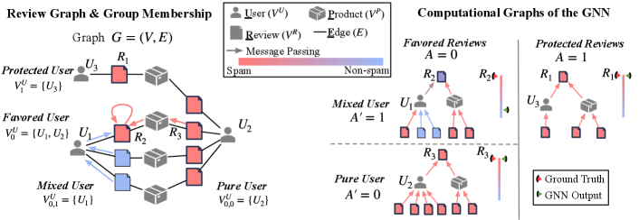
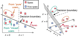
Refer to caption — Figure 1. Problem setting and challenges. Left: a toy example of the review graph $\mathcal{G}$ and group membership. GNN infers the suspiciousness of reviews (e.g., $R_{2}$ ) by passing and aggregating the messages from its neighbors. Right: computational graphs of GNN on spam reviews from different groups and subgroups. GNN unfairly assigns a low suspiciousness to spam $R_{2}$ posted by mixed user $U_{1}$ , due to the aggregation of messages coming from other non-spams posted by $U_{1}$ .

In fact, maintaining fairness between groups of users categorized only by node degree is imprecise. The detection fairness essentially depends on if two users have the same capability to hide their spamming reviews from their normal reviews. Two “favored” users can receive different treatment from the detector due to their heterogeneous behaviors, i.e., the various proportions of spams to non-spams across users. As for “protected” users, they post only a few reviews but belong to the same class, reflecting homogeneous user behaviors, whose reviews are treated equally by the detector. In order to ensure fairness in spam detection, the heterogeneous behavior of “favored” users must be accurately described by an additional sensitive attribute $A^{\prime}$ to indicate if their reviews are from the same class. In Fig. 1, user $U_{1}$ , named as the “mixed” user, denoted by $A^{\prime}=1$ , posts both spams and non-spams where spams deceive the detector by aggregating messages from non-spams. $U_{2}$ , named as the “pure” user, denoted by $A^{\prime}=0$ , posts only spams and thus receives no messages from non-spams to lower the suspiciousness calculated by the GNN model.. In order to get higher accuracy on the favored group, GNN will unfairly target spam reviews posted by pure users like $U_{2}$ since they are easier to detect. Once we let the spams from “mixed” users are easy to be caught as well, GNN will have better performance on detecting spams from “mixed” users without harming the detection accuracy of spams from “pure” user. As a result, distinguishing mixed users from pure users is crucial. Solving this problem involves three main challenges:

Define the subgroup structure. Most of the previous work studied the fairness problem with well-defined sensitive attributes. Studies including (ustun2019fairness; kearns2018preventing) utilize observable sensitive attributes and their combinations to divide the dataset into various groups. Others (celis2021fair; awasthi2020equalized; mehrotra2021mitigating) consider the fairness problem with unobserved or noisy sensitive attributes. In (chen2019fairness), researchers built probabilistic models to approximate the value of any well-defined sensitive attribute by using proxy information. For example, it infers race from the last name and geolocation. All of these methods are implemented on the I.I.D vector data with well-defined sensitive attributes. Unlike the above works, we enhance fairness by discovering a novel structural-based sensitive attribute $A^{\prime}$ and its approximation. Additionally, sensitive attributes in previous works (dwork2012fairness; hardt2016equality; zemel2013learning) have been treated as data characteristics, which are not determined by ground truth labels. We are looking for an undefined sensitive attribute $A^{\prime}$ that is both specific to graph-based spam detection and related to the ground truth of reviews.

Infer unknown subgroup membership. We hypothesize that inferring $A^{\prime}$ helps resolve the unfairness among groups. Indicating a user’s heterogeneous behavior by the subgroup indicator $A^{\prime}$ , either mixed or pure, helps clarify what users from the “favored” group genuinely benefit from their non-spams. In this case, GNN can use the inferred indicator $A^{\prime}$ to strike a more equitable detection on spams posted by users from the “favored” group and then promote group fairness. (See Fig. 2). Nevertheless, the indicator $A^{\prime}$ relates to the ground truth labels, which are unobservable for the test data and need to be inferred. Even for the training data, labeling sufficient data and precisely identifying spams are great challenges that are expensive and time-consuming (qiu2020adaptive; tan2013unik; tian2020non).
Promote group fairness through subgroup information. Considering fairness towards multiple sensitive attributes, the related works (kearns2018preventing; ustun2019fairness) formulated the optimization problem with several fairness constraints for each group of combinations. These sensitive attributes must be precise and discrete in order to categorize data and ensure that those being discriminated against are fairly treated. However, these premises are inapplicable to our inferred subgroup membership indicator $A^{\prime}$ , which is probabilistic rather than deterministic. Meanwhile, constraints derived from thresholding noisy sensitive attributes can deteriorate optimization algorithms. Fairness optimization is highly sensitive to group separation, so we avoid setting an uncertain threshold for converting membership from a probability to a concrete group.

The main contributions of this work are as follows:

[leftmargin=*]
•

In addition to well-known sensitive attributes, i.e., user node degree (burkholder2021certification) or node attributes (bose2019compositional; dai2021say; wu2021learning), we first define a new structural-based and label-related sensitive attribute $A^{\prime}$ in the fair spam detection task on graph.
•

We propose another GNN $g_{\bt}$ to infer the probability distribution of $A^{\prime}$ for the test users who have unlabelled reviews (i.e., unobserved user behaviors). Due to the insufficient training examples for the “favored” group and the “mixed” subgroup, we propose two fairness-aware data augmentation methods to synthesize nodes and edges. GNN will generate less biased representations of the minority groups and subgroups by using the re-balanced training datasets.
•

Rather than converting the estimated probability distribution of $A^{\prime}$ into concrete groups by any uncertain threshold, a joint training method is designed to let the detector $f_{\bw}$ directly use the inferred $A^{\prime}$ . Our proposed method is evaluated on three real-world Yelp datasets. The results demonstrate the unfairness inside the “favored” group and show group fairness can be enhanced by introducing the subgroup membership indicator $A^{\prime}$ . We show that regardless of what thresholds are used to split the group regarding $A$ , our joint method promotes group fairness by accurately inferring the distribution of $A^{\prime}$ during model training.

2. Preliminaries

2.1. Spam detection based on GNN

Our spam detection is on the review-graph defined as $\mathcal{G}=(\mathcal{V},\mathcal{E})$ , where $\mathcal{V}=\{v_{1},\dots,v_{N}\}$ denotes the set of nodes and $\mathcal{E}\subseteq\mathcal{V}\times\mathcal{V}$ denotes the set of undirected edges. Each node $v_{i}\in\mathcal{V}$ has a feature vector $\mathbf{x}_{i}$ with node index $i$ . $\mathcal{G}$ contains three types of nodes: user, review, and product, where each node is from only one of the three types (see the example in Fig. 1 left). Let $\mathcal{V}^{U},\mathcal{V}^{R}$ and $\mathcal{V}^{P}$ denote the sets of user, review, and product nodes, respectively. $v_{i}$ has a set of neighboring nodes denoted by $\mathcal{N}(i)=\{v_{j}\in\mathcal{V}|e_{i,j}\in\mathcal{E}\}$ . The work focuses on detecting spammy users and reviews, and the task is essentially a node classification problem. GNN (kipf2016semi) is the state-of-the-art method for node classification (wu2020comprehensive). For our GNN detector $f_{\bw}(\cdot)$ , let $\mathbf{h}_{i}^{(l)}$ be the learned representation of node $v_{i}$ at layer $l$ , where $l=1,\dots L$ :

(1)

\mathbf{h}_{i}^{(l)}=\text{UPDATE}\left(\text{AGGREGATE}\left(\left\{\mathbf{h}_{i}^{(l-1)}\right\}\bigcup\left\{{\mathbf{h}_{j}^{(l-1)}\mid j\in\mathcal{N}(i)}\right\}\right),\bw^{(l)}\right),

where AGGREGATE takes the mean over $\mathbf{h}_{i}^{(l)}$ and messages passed from its neighboring nodes. UPDATE contains an affine mapping with parameters $\boldsymbol{W}^{(l)}$ followed by a nonlinear mapping (ReLU in $l=1,\dots,L-1$ and Sigmoid in $l=L$ ). The input vector $\mathbf{x}_{i}=\mathbf{h}_{i}^{(0)}$ is the representation at layer 0. $\hat{y}_{i}=\mathbf{h}_{i}^{(L)}\in\mathbb{R}$ denotes the prediction probability of $v_{i}$ being spam. We minimize the cross-entropy loss for the training node set $\mathcal{V}^{\text{Tr}}$ :

(2)

\mathcal{L}(\boldsymbol{W};\mathcal{G})=\frac{1}{|\mathcal{V}^{\text{Tr}}|}\sum_{v_{i}\in\mathcal{V}^{\text{Tr}}}\left(-y_{i}\cdot\log\hat{y}_{i}-(1-y_{i})\cdot\log(1-\hat{y}_{i})\right),

where $y_{i}\in\{0,1\}$ is the class for $v_{i}$ . $\bw$ represents a collection of parameters in all the layers $L$ . The main notations are in Table 1.

2.2. Fairness regularizer

Group. We split users $\mathcal{V}^{U}$ into the protected group $\mathcal{V}^{U}_{1}$ whose degree is smaller than the $p$ -th percentile of all the users’ degrees, and the favored group $\mathcal{V}^{U}_{0}$ for the remaining users (see Fig. 1 left). The subscript denotes the value of $A$ . The review nodes $\mathcal{V}^{R}$ are divided into $\mathcal{V}^{R}_{1}$ and $\mathcal{V}^{R}_{0}$ following the group of their associated users. The fairness of the GNN detector is evaluated by the detection accuracies between two groups of spams $\mathcal{V}^{R}_{0}$ and $\mathcal{V}_{1}^{R}$ .

Fairness regularizer. Ranking-based metrics like NDCG are appropriate to evaluate the detector’s accuracy, as the highly skewed class distribution: most reviews are genuine. A larger NDCG score indicates that spams are ranked higher than non-spams, and a detector is more precise. NDCG can also be evaluated on the two groups $\mathcal{V}^{R}_{0}$ and $\mathcal{V}^{R}_{1}$ , separately. Hence, the group fairness can be evaluated by the NDCG gap between $\mathcal{V}^{R}_{0}$ and $\mathcal{V}^{R}_{1}$ , denoted as $\Delta_{\text{NDCG}}$ . In fact, NDCG on the “favored” group $\mathcal{V}^{R}_{0}$ is always lower than that on the $\mathcal{V}^{R}_{1}$ , since the detector performs preciser on group $\mathcal{V}^{R}_{1}$ . For reducing $\Delta_{\text{NDCG}}$ by promoting the NDCG of $\mathcal{V}^{R}_{0}$ without hurting that of $\mathcal{V}^{R}_{1}$ , our detector $f_{\boldsymbol{W}}(\cdot)$ starts with a fairness regularizer $\mathcal{R}_{\text{fair}}$ which takes negative NDCG of $\mathcal{V}^{R}_{0}$ . We adopt a differentiable surrogate NDCG (burkholder2021certification) for $\mathcal{R}_{\text{fair}}$

(3)		$\displaystyle\mathcal{R}_{\text{fair}}(\boldsymbol{W};\mathcal{G})$	$\displaystyle=-\frac{1}{Z_{0}}\sum_{i,j:y_{i}<y_{j}\atop v_{i},v_{j}\in\mathcal{V}^{R}_{0}\cap\mathcal{V}^{\text{Tr}}}\log\left(1+\exp\left(\mathbf{h}_{j}^{(L)}-\mathbf{h}_{i}^{(L)}\right)\right),$
(4)		$\displaystyle\mathcal{L}_{\text{GNN}}(\boldsymbol{W};\mathcal{G})$	$\displaystyle=\mathcal{L}(\boldsymbol{W};\mathcal{G})+\lambda\cdot\mathcal{R}_{\text{fair}}(\boldsymbol{W};\mathcal{G}),$

where $Z_{0}$ is the total number of pairs of spams and non-spams in the training $\mathcal{V}^{R}_{0}$ . $\mathcal{L}_{\text{GNN}}$ is the objective function for training $f_{\boldsymbol{W}}(\cdot)$ by adding $\mathcal{R}_{\text{fair}}$ to $\mathcal{L}(\boldsymbol{W};\mathcal{G})$ in Eq. (2). $\lambda>0$ is the importance of the fairness regularizer. Note that the fairness regularizer $\mathcal{R}_{\text{fair}}$ regularizes all the models referred to in this paper below.

Table 1. Notations and definitions.

Graph notations
Notations	Definitions
$\mathcal{G}$	Review graph
$\mathcal{V},\mathcal{E}$	Nodes and Edges of graph $\mathcal{G}$
$\mathbf{x}_{i},y_{i}$	Feature and label of node $v_{i}$
$\mathcal{N}(i)$	Set of direct neighbors of $v_{i}$
$\|\mathcal{V}\|$	Cardinality of a set $\mathcal{V}$
$\mathcal{V}^{\text{Tr}},\mathcal{V}^{\text{Te}}$	Training nodes and test nodes
$\mathcal{V}^{U},\mathcal{V}^{R},\mathcal{V}^{P}$	User, review, and product nodes
Group notations
$A,A^{\prime}$	Binary sensitive attributes (0/1)
$\mathcal{V}^{R}_{a},\mathcal{V}^{U}_{a}$	Review and user nodes from group of $A=a$
$\mathcal{V}^{R}_{a,a^{\prime}},\mathcal{V}^{U}_{a,a^{\prime}}$	Review and user nodes from group of $A=a$ and $A^{\prime}=a^{\prime}$
Model notations
$f_{\boldsymbol{W}}(\cdot),g_{\boldsymbol{\theta}}(\cdot)$	GNNs with parameters $\boldsymbol{W}$ and $\boldsymbol{\theta}$
$\hat{y}_{i},\hat{A}^{\prime}_{i}$	Output of $f_{\boldsymbol{W}}(\cdot),g_{\boldsymbol{\theta}}(\cdot)$ for $v_{i}$
$\textbf{h}_{i}^{(l)}$	Representation of $v_{i}$ on layer $l$
$\tilde{\mathbf{x}}_{ij}$	Synthetic node by mixing-up $v_{i}$ and $v_{j}$
$\tilde{y}_{ij}$	Label for the synthetic node $\tilde{\mathbf{x}}_{ij}$

3. EXPERIMENTS

We seek to answer the following research questions:
RQ1: Do fairness issues exist between the “favored” and the “protected” groups, and between the “mixed” and the “pure” groups when using a GNN spam detector? Will the inferred $A^{\prime}$ improve the group fairness?
RQ2: How to infer the subgroup memberships $A^{\prime}$ defined in Eq. (LABEL:eq._definition_for_A') with a shortage of training examples?
RQ3: Can the joint training method simultaneously promote the AUC of predicted $A^{\prime}$ and group fairness?
RQ4: Does the accuracy of predicting $A^{\prime}$ contribute to the improvement in group fairness?

3.1. Experimental Settings

Datasets. We used three Yelp review datasets (“Chi”, “NYC”, and “Zip” for short, see Table 2) which are commonly used in previous spam detection tasks (burkholder2021certification; dou2020enhancing). For the cutoff degree of user nodes ( $p$ -th percentile in Section 2.2), we treat $p\in\{20,15,10\}$ as a hyper-parameter distinguishing favored (top $p\%$ high-degree users, $A=0$ ) from protected groups (the remaining users, $A=1$ ). Reviews have the same value of $A$ as their associated users. The favored users are further split into pure ( $A^{\prime}=0$ ) and mixed ( $A^{\prime}=1$ ) users following Eq. (LABEL:eq._definition_for_A'). Users are divided into training ( $30\%$ ), validation ( $10\%$ ), and test ( $60\%$ ) sets with their associated reviews.

Table 2. Statistics of the datasets. We list the numbers of products, reviews, and users with the proportion of favored users/reviews (

\%\mathcal{V}_{0}^{U}

\%\mathcal{V}_{0}^{R}

) and mixed users/reviews (

\%\mathcal{V}_{0,1}^{U}

\%\mathcal{V}_{0,1}^{R}

) under 20-th, 15-th, and 10-th percentile (PC) of cutoff degree of the user groups. The last column gives the ratio of spam in the group of

A=0

A=1

\multirow2*Name	Data Statistics						\multirow2* $\frac{P(Y=1\|A=0)}{P(Y=1\|A=1)}$
	$\|\mathcal{V}^{P}\|$	$\|\mathcal{V}^{R}\|$			$\|\mathcal{V}^{U}\|$
\multirow5*Chi	\multirow5* $201$	$67,395$			$38,063$
		PC	$\%\mathcal{V}^{R}_{0}$	$\%\mathcal{V}^{R}_{0,1}$	$\%\mathcal{V}^{U}_{0}$	$\%\mathcal{V}^{U}_{0,1}$
		20th	$13.581\%$	$0.116\%$	$1.781\%$	$0.011\%$	$0.0438$
		15th	$18.687\%$	$0.129\%$	$3.003\%$	$0.026\%$	$0.0125$
		10th	$27.003\%$	$0.224\%$	$5.735\%$	$0.058\%$	$0.0282$
\multirow5*NYC	\multirow5* $923$	$358,911$			$160,220$
		PC	$\%\mathcal{V}^{R}_{0}$	$\%\mathcal{V}^{R}_{0,1}$	$\%\mathcal{V}^{U}_{0}$	$\%\mathcal{V}^{U}_{0,1}$
		20th	$12.665\%$	$0.193\%$	$0.760\%$	$0.009\%$	$0.0479$
		15th	$16.264\%$	$0.258\%$	$1.171\%$	$0.018\%$	$0.0289$
		10th	$23.096\%$	$0.360\%$	$2.260\%$	$0.034\%$	$0.0420$
\multirow5*Zip	\multirow5* $5,044$	$608,598$			$260,277$
		PC	$\%\mathcal{V}^{R}_{0}$	$\%\mathcal{V}^{R}_{0,1}$	$\%\mathcal{V}^{U}_{0}$	$\%\mathcal{V}^{U}_{0,1}$
		20th	$6.859\%$	$0.050\%$	$0.272\%$	$0.002\%$	$0.0426$
		15th	$15.658\%$	$0.145\%$	$1.020\%$	$0.009\%$	$0.0139$
		10th	$22.342\%$	$0.278\%$	$1.968\%$	$0.018\%$	$0.0241$

Evaluation Metrics. (1) NDCG is to evaluate the detector’s accuracy, where a higher NDCG means that the detector tends to assign a higher suspiciousness to spams than non-spams. (2) To evaluate the ranking of spams within the group of $A=0$ , a metric called “Average False Ranking Ratio” is proposed to measure the average of relative ranking between spams from mixed and pure users

(5)

\text{AFRR}_{A^{\prime}}=\frac{1}{Z}\sum_{y_{j}=1\atop v_{j}\in\mathcal{V}^{R}_{0,A^{\prime}}}\frac{\sum_{i=1}^{|\mathcal{V}^{R}_{0}|}\mathbbm{1}\left[\hat{y}_{i}>\hat{y}_{j},y_{i}=0\right]}{\sum_{i=1}^{|\mathcal{V}^{R}_{0}|}\mathbbm{1}[y_{i}=0]},\quad A^{\prime}\in\{0,1\}

where $A^{\prime}\in\{0,1\}$ denotes the subgroup membership. $Z$ is the number of spams from a subgroup. $\mathcal{V}^{R}_{0,A^{\prime}}$ denotes the reviews from a subgroup users. The ratio in the above equation calculates the proportion of non-spams ranked higher than spams over all the non-spams from the group of $A=0$ . The lower the AFRR, the fewer non-spams ranked higher than spams. Compared to NDCG, AFRR considers the non-spams across different subgroups and ignores the relative ranking of spams from the other subgroup. (3) AUC is to evaluate the performance of $g_{\bt}$ in predicting $A^{\prime}$ . The larger the AUC value, the more accurate $A^{\prime}$ given by $g_{\bt}$ .

Methods compared. Joint+GNN- $\mathbf{S_{1}^{\textbf{Tr}}}$ denotes our method: Joint is the joint training for two GNNs ( $f_{\bw}$ and $g_{\bt}$ in Section LABEL:sec_3.3:_joint_training), GNN- $\mathbf{S_{1}^{\textbf{Tr}}}$ is a GNN with our mixup method in Eq. (LABEL:eq:_mixup_second_node). “a+b” denotes a setting: “a” is one of a method for obtaining the value of $A^{\prime}$ ; “b” is a spam detector.

Baselines for obtaining the value of $A^{\prime}$ (selections for “a”):

[leftmargin=*]
•

w/o: has no definition of $A^{\prime}$ .
•

Random: randomly assigns $1/0$ to $A^{\prime}$ .
•

GT: assigns the ground truth of $A^{\prime}$ for users, which is the ideal case, as $A^{\prime}$ is unknown.
•

Pre-trained: is a variant of Joint that pre-training $g_{\boldsymbol{\theta}}$ to infer $A^{\prime}$ and fixes the inferred $A^{\prime}$ when training $f_{\boldsymbol{W}}$ .

Baselines for the spam detectors (selections for “b”):

[leftmargin=*]
•

FairGNN (dai2021say): is an adversarial method to get fair predictions for all groups defined by the known $A$ .
•

EDITS (dong2022edits): modifies the node attribute and the graph structure to debias the graph. FairGNN and EDITS consider $A$ as a known sensitive attribute and exclude any information about $A^{\prime}$ defined by our work.
•

GNN: is the vanilla GNN.
•

GNN- $\mathbf{S_{0}^{\textbf{Te}}}$ is a GNN with the mixup Case 2 in Eq. (LABEL:eq:_mixup_second_node).
•

GNN- $\mathbf{S_{1}^{\textbf{Te}}}$ is a GNN with the mixup Case 3 in Eq. (LABEL:eq:_mixup_second_node).

We set $T=300$ , $\lambda=5$ , $\beta_{1}=\beta_{2}=0.001$ , weight decay $=0.0001$ for both $f_{\boldsymbol{W}}$ and $g_{\boldsymbol{\theta}}$ in Algorithm LABEL:alg:_joint_train, mixup weight $\alpha=0.8$ . We have 10 training-validation-test splits of the three datasets. The following results are based on the aggregated performance on all splits.

Table 3. NDCG values for the outputs of spam detectors on three Yelp datasets with

20

-percentile of user degree as a cutoff for group of

A

. Shown are the mean and standard deviation of

\Delta_{\text{NDCG}}

over all 10 splits. “*” denotes our method. The lower the

\Delta_{\text{NDCG}}

, the fairer the model.

Detector	Metrics(%)	Chi			NYC			Zip
\multirow3*FairGNN (dai2021say)	NDCG( $\mathcal{V}^{R}$ )	86.2 $\pm$ 0.1			85.9 $\pm$ 0.0			89.6 $\pm$ 0.5
	NDCG( $\mathcal{V}^{R}_{1}$ )	86.2 $\pm$ 0.1			86.0 $\pm$ 0.0			89.6 $\pm$ 0.4
\rowcolorgray!20 \cellcolorwhite	$\Delta_{\text{NDCG}}$	53.7 $\pm$ 2.1			20.7 $\pm$ 1.1			36.4 $\pm$ 4.6
\multirow3*EDITS (dong2022edits)	NDCG( $\mathcal{V}^{R}$ )	84.3 $\pm$ 0.3			84.9 $\pm$ 0.1			89.2 $\pm$ 0.0
	NDCG( $\mathcal{V}^{R}_{1}$ )	84.3 $\pm$ 0.3			85.1 $\pm$ 0.1			89.3 $\pm$ 0.0
\rowcolorgray!20 \cellcolorwhite	$\Delta_{\text{NDCG}}$	50.9 $\pm$ 2.3			32.7 $\pm$ 1.5			39.4 $\pm$ 10.6
\multirow2*Detector	\multirow2*Metrics(%)	GNN $(g_{\boldsymbol{\theta}})$			GNN $(g_{\boldsymbol{\theta}})$			GNN $(g_{\boldsymbol{\theta}})$
		w/o	Pre-trained	Joint*	w/o	Pre-trained	Joint*	w/o	Pre-trained	Joint*
\multirow3*GNN	NDCG( $\mathcal{V}^{R}$ )	84.5 $\pm$ 0.9	83.2 $\pm$ 1.5	83.3 $\pm$ 2.2	85.2 $\pm$ 0.8	85.1 $\pm$ 0.8	85.2 $\pm$ 0.5	88.4 $\pm$ 1.4	87.6 $\pm$ 1.5	88.6 $\pm$ 1.0
	NDCG( $\mathcal{V}^{R}_{1}$ )	84.7 $\pm$ 0.9	83.5 $\pm$ 1.3	83.6 $\pm$ 2.1	85.1 $\pm$ 0.8	85.3 $\pm$ 0.8	85.2 $\pm$ 0.5	88.4 $\pm$ 1.4	87.6 $\pm$ 1.5	88.6 $\pm$ 1.0
\rowcolorgray!20 \cellcolorwhite	$\Delta_{\text{NDCG}}$	51.2 $\pm$ 2.1	51.0 $\pm$ 3.0	50.7 $\pm$ 3.5	21.9 $\pm$ 7.0	21.8 $\pm$ 7.8	21.3 $\pm$ 8.9	36.3 $\pm$ 10.4	34.3 $\pm$ 10.8	34.8 $\pm$ 11.1
\multirow3GNN- $\mathbf{S_{1}^{\textbf{Tr}}}$	NDCG( $\mathcal{V}^{R}$ )	85.6 $\pm$ 0.7	85.8 $\pm$ 0.5	85.6 $\pm$ 0.8	85.8 $\pm$ 0.1	85.9 $\pm$ 0.0	85.9 $\pm$ 0.0	89.7 $\pm$ 0.2	89.7 $\pm$ 0.1	89.6 $\pm$ 0.1
	NDCG( $\mathcal{V}^{R}_{1}$ )	85.6 $\pm$ 0.7	85.8 $\pm$ 0.5	85.7 $\pm$ 0.8	85.9 $\pm$ 0.0	86.0 $\pm$ 0.0	86.0 $\pm$ 0.0	89.7 $\pm$ 0.2	89.7 $\pm$ 0.1	89.6 $\pm$ 0.1
\rowcolorgray!20 \cellcolorwhite	$\Delta_{\text{NDCG}}$	51.6 $\pm$ 0.9	50.3 $\pm$ 1.0	50.1 $\pm$ 1.0	19.1 $\pm$ 5.5	19.0 $\pm$ 5.2	17.9 $\pm$ 6.1	38.7 $\pm$ 7.2	36.0 $\pm$ 9.0	34.3 $\pm$ 11.5
\multirow3*GNN- $\mathbf{S_{0}^{\textbf{Te}}}$	NDCG( $\mathcal{V}^{R}$ )	85.1 $\pm$ 0.7	85.3 $\pm$ 1.4	85.2 $\pm$ 1.4	85.3 $\pm$ 0.6	85.4 $\pm$ 0.5	85.4 $\pm$ 0.4	89.4 $\pm$ 0.6	89.6 $\pm$ 0.1	89.0 $\pm$ 0.06
	NDCG( $\mathcal{V}^{R}_{1}$ )	85.2 $\pm$ 0.8	83.4 $\pm$ 1.3	83.5 $\pm$ 1.3	85.2 $\pm$ 0.6	85.5 $\pm$ 0.4	85.5 $\pm$ 0.4	89.4 $\pm$ 0.06	89.0 $\pm$ 0.01	89.1 $\pm$ 0.06
\rowcolorgray!20 \cellcolorwhite	$\Delta_{\text{NDCG}}$	51.2 $\pm$ 1.5	50.9 $\pm$ 2.4	50.9 $\pm$ 2.3	21.9 $\pm$ 6.9	21.9 $\pm$ 6.3	20.9 $\pm$ 9.4	38.9 $\pm$ 7.6	36.9 $\pm$ 9.5	34.9 $\pm$ 11.0
\multirow3*GNN- $\mathbf{S_{1}^{\textbf{Te}}}$	NDCG( $\mathcal{V}^{R}$ )	84.7 $\pm$ 1.3	83.7 $\pm$ 0.9	83.1 $\pm$ 0.9	85.7 $\pm$ 0.1	85.8 $\pm$ 0.1	85.8 $\pm$ 0.2	89.6 $\pm$ 0.3	89.6 $\pm$ 0.1	89.5 $\pm$ 0.3
	NDCG( $\mathcal{V}^{R}_{1}$ )	84.8 $\pm$ 1.3	83.9 $\pm$ 0.9	83.4 $\pm$ 0.9	85.8 $\pm$ 0.1	85.8 $\pm$ 0.1	85.8 $\pm$ 0.1	89.6 $\pm$ 0.3	89.6 $\pm$ 0.1	89.5 $\pm$ 0.3
\rowcolorgray!20 \cellcolorwhite	$\Delta_{\text{NDCG}}$	51.3 $\pm$ 0.6	50.8 $\pm$ 0.6	50.2 $\pm$ 1.0	21.0 $\pm$ 5.4	19.8 $\pm$ 5.4	19.3 $\pm$ 6.8	38.7 $\pm$ 7.2	36.2 $\pm$ 9.5	34.6 $\pm$ 11.4

Table 4. NDCG values for the outputs of detectors on Yelp datasets with

15

-percentile of user degree as a cutoff for group of

A

Detector	Metrics(%)	Chi			NYC			Zip
\multirow3*FairGNN (dai2021say)	NDCG( $\mathcal{V}^{R}$ )	86.2 $\pm$ 0.2			85.9 $\pm$ 0.1			89.9 $\pm$ 0.0
	NDCG( $\mathcal{V}^{R}_{1}$ )	86.3 $\pm$ 0.2			86.0 $\pm$ 0.1			90.0 $\pm$ 0.0
\rowcolorgray!20 \cellcolorwhite	$\Delta_{\text{NDCG}}$	45.8 $\pm$ 1.7			20.0 $\pm$ 2.4			31.0 $\pm$ 2.7
\multirow3*EDITS (dong2022edits)	NDCG( $\mathcal{V}^{R}$ )	84.3 $\pm$ 0.2			85.0 $\pm$ 0.1			89.2 $\pm$ 0.0
	NDCG( $\mathcal{V}^{R}_{1}$ )	84.4 $\pm$ 0.2			85.1 $\pm$ 0.1			89.3 $\pm$ 0.0
\rowcolorgray!20 \cellcolorwhite	$\Delta_{\text{NDCG}}$	43.8 $\pm$ 2.6			32.4 $\pm$ 1.5			34.4 $\pm$ 3.5
\multirow2*Detector	\multirow2*Metrics(%)	GNN $(g_{\boldsymbol{\theta}})$			GNN $(g_{\boldsymbol{\theta}})$			GNN $(g_{\boldsymbol{\theta}})$
		w/o	Pre-trained	Joint*	w/o	Pre-trained	Joint*	w/o	Pre-trained	Joint*
\multirow3*GNN	NDCG( $\mathcal{V}^{R}$ )	84.3 $\pm$ 1.3	84.3 $\pm$ 0.9	84.4 $\pm$ 0.9	85.7 $\pm$ 0.2	84.5 $\pm$ 0.4	84.6 $\pm$ 0.5	89.5 $\pm$ 0.2	88.9 $\pm$ 0.6	88.9 $\pm$ 0.6
	NDCG( $\mathcal{V}^{R}_{1}$ )	84.6 $\pm$ 1.1	84.7 $\pm$ 0.7	84.8 $\pm$ 0.7	85.8 $\pm$ 0.2	84.6 $\pm$ 0.4	84.6 $\pm$ 0.5	89.5 $\pm$ 0.2	88.9 $\pm$ 0.6	88.9 $\pm$ 0.7
\rowcolorgray!20 \cellcolorwhite	$\Delta_{\text{NDCG}}$	41.8 $\pm$ 2.4	40.9 $\pm$ 3.7	40.9 $\pm$ 4.0	16.3 $\pm$ 3.9	15.8 $\pm$ 2.7	15.2 $\pm$ 6.1	26.1 $\pm$ 3.4	26.6 $\pm$ 2.5	25.9 $\pm$ 2.7
\multirow3GNN- $\mathbf{S_{1}^{\textbf{Tr}}}$	NDCG( $\mathcal{V}^{R}$ )	86.0 $\pm$ 0.4	85.9 $\pm$ 0.3	85.9 $\pm$ 0.2	85.9 $\pm$ 0.1	85.9 $\pm$ 0.1	85.9 $\pm$ 0.1	89.7 $\pm$ 0.1	89.9 $\pm$ 0.0	87.9 $\pm$ 2.1
	NDCG( $\mathcal{V}^{R}_{1}$ )	86.0 $\pm$ 0.4	86.0 $\pm$ 0.3	86.0 $\pm$ 0.2	85.9 $\pm$ 0.1	85.9 $\pm$ 0.1	85.9 $\pm$ 0.1	89.8 $\pm$ 0.1	89.9 $\pm$ 0.0	87.9 $\pm$ 2.1
\rowcolorgray!20 \cellcolorwhite	$\Delta_{\text{NDCG}}$	43.2 $\pm$ 2.0	41.9 $\pm$ 5.8	40.5 $\pm$ 5.1	16.5 $\pm$ 3.8	15.6 $\pm$ 2.9	15.6 $\pm$ 3.6	26.4 $\pm$ 3.3	27.0 $\pm$ 3.2	22.7 $\pm$ 4.2
\multirow3*GNN- $\mathbf{S_{0}^{\textbf{Te}}}$	NDCG( $\mathcal{V}^{R}$ )	84.4 $\pm$ 1.5	84.3 $\pm$ 1.1	84.4 $\pm$ 0.9	85.8 $\pm$ 0.2	84.7 $\pm$ 0.4	84.7 $\pm$ 0.4	89.4 $\pm$ 0.2	89.1 $\pm$ 0.6	89.1 $\pm$ 0.6
	NDCG( $\mathcal{V}^{R}_{1}$ )	84.7 $\pm$ 1.1	84.6 $\pm$ 0.9	84.8 $\pm$ 0.	85.9 $\pm$ 0.2	84.7 $\pm$ 0.5	84.7 $\pm$ 0.5	89.5 $\pm$ 0.2	89.1 $\pm$ 0.6	89.2 $\pm$ 0.6
\rowcolorgray!20 \cellcolorwhite	$\Delta_{\text{NDCG}}$	43.4 $\pm$ 2.4	41.7 $\pm$ 4.6	41.1 $\pm$ 4.2	16.6 $\pm$ 4.1	15.7 $\pm$ 3.0	15.6 $\pm$ 3.6	26.2 $\pm$ 4.0	27.2 $\pm$ 3.2	25.3 $\pm$ 2.7
\multirow3*GNN- $\mathbf{S_{1}^{\textbf{Te}}}$	NDCG( $\mathcal{V}^{R}$ )	85.9 $\pm$ 0.5	85.8 $\pm$ 0.3	85.9 $\pm$ 0.3	85.8 $\pm$ 0.1	85.4 $\pm$ 0.3	85.5 $\pm$ 0.3	89.8 $\pm$ 0.1	89.9 $\pm$ 0.1	89.9 $\pm$ 0.1
	NDCG( $\mathcal{V}^{R}_{1}$ )	85.9 $\pm$ 0.5	85.9 $\pm$ 0.3	85.9 $\pm$ 0.3	85.9 $\pm$ 0.2	85.5 $\pm$ 0.3	85.5 $\pm$ 0.3	89.8 $\pm$ 0.1	89.9 $\pm$ 0.1	89.9 $\pm$ 0.1
\rowcolorgray!20 \cellcolorwhite	$\Delta_{\text{NDCG}}$	42.6 $\pm$ 2.8	40.7 $\pm$ 3.7	40.7 $\pm$ 3.7	16.0 $\pm$ 3.9	15.5 $\pm$ 3.0	15.6 $\pm$ 3.3	26.1 $\pm$ 3.5	27.1 $\pm$ 2.4	24.9 $\pm$ 2.7

Table 5. NDCG values for the outputs of detectors on Yelp datasets with

10

-percentile of user degree as a cutoff for group of

A

Detector	Metrics(%)	Chi			NYC			Zip
\multirow3*FairGNN (dai2021say)	NDCG( $\mathcal{V}^{R}$ )	86.2 $\pm$ 0.2			85.9 $\pm$ 0.1			89.9 $\pm$ 0.0
	NDCG( $\mathcal{V}^{R}_{1}$ )	86.4 $\pm$ 0.2			86.0 $\pm$ 0.1			90.0 $\pm$ 0.0
\rowcolorgray!20 \cellcolorwhite	$\Delta_{\text{NDCG}}$	33.8 $\pm$ 5.4			22.4 $\pm$ 1.9			24.8 $\pm$ 1.6
\multirow3*EDITS (dong2022edits)	NDCG( $\mathcal{V}^{R}$ )	84.3 $\pm$ 0.2			85.0 $\pm$ 0.1			89.2 $\pm$ 0.0
	NDCG( $\mathcal{V}^{R}_{1}$ )	84.5 $\pm$ 0.2			85.2 $\pm$ 0.1			89.4 $\pm$ 0.0
\rowcolorgray!20 \cellcolorwhite	$\Delta_{\text{NDCG}}$	37.1 $\pm$ 2.0			30.0 $\pm$ 1.2			28.9 $\pm$ 1.3
\multirow2*Detector	\multirow2*Metrics(%)	GNN $(g_{\boldsymbol{\theta}})$			GNN $(g_{\boldsymbol{\theta}})$			GNN $(g_{\boldsymbol{\theta}})$
		w/o	Pre-trained	Joint*	w/o	Pre-trained	Joint*	w/o	Pre-trained	Joint*
\multirow3*GNN	NDCG( $\mathcal{V}^{R}$ )	85.4 $\pm$ 0.5	84.7 $\pm$ 1.3	84.9 $\pm$ 1.4	84.8 $\pm$ 0.4	84.5 $\pm$ 0.3	84.6 $\pm$ 0.4	89.7 $\pm$ 0.3	89.6 $\pm$ 0.6	88.9 $\pm$ 0.6
	NDCG( $\mathcal{V}^{R}_{1}$ )	85.7 $\pm$ 0.4	85.3 $\pm$ 0.8	85.4 $\pm$ 0.9	84.8 $\pm$ 0.4	84.6 $\pm$ 0.3	84.7 $\pm$ 0.4	89.8 $\pm$ 0.3	89.6 $\pm$ 0.6	89.8 $\pm$ 0.4
\rowcolorgray!20 \cellcolorwhite	$\Delta_{\text{NDCG}}$	34.7 $\pm$ 1.5	33.9 $\pm$ 2.5	34.7 $\pm$ 1.5	19.7 $\pm$ 1.6	19.1 $\pm$ 1.6	18.7 $\pm$ 2.0	25.0 $\pm$ 1.8	23.7 $\pm$ 1.7	23.6 $\pm$ 1.7
\multirow3GNN- $\mathbf{S_{1}^{\textbf{Tr}}}$	NDCG( $\mathcal{V}^{R}$ )	85.9 $\pm$ 0.4	86.1 $\pm$ 0.2	86.1 $\pm$ 0.2	85.9 $\pm$ 0.1	85.9 $\pm$ 0.1	85.9 $\pm$ 0.1	89.7 $\pm$ 0.1	89.9 $\pm$ 0.0	89.9 $\pm$ 0.0
	NDCG( $\mathcal{V}^{R}_{1}$ )	85.9 $\pm$ 0.4	86.2 $\pm$ 0.2	86.2 $\pm$ 0.2	86.0 $\pm$ 0.1	86.0 $\pm$ 0.1	86.0 $\pm$ 0.1	89.8 $\pm$ 0.1	90.0 $\pm$ 0.0	90.0 $\pm$ 0.0
\rowcolorgray!20 \cellcolorwhite	$\Delta_{\text{NDCG}}$	34.1 $\pm$ 4.6	33.7 $\pm$ 3.0	33.2 $\pm$ 2.6	19.1 $\pm$ 1.9	16.8 $\pm$ 1.5	16.6 $\pm$ 1.9	25.1 $\pm$ 1.6	23.4 $\pm$ 1.6	23.3 $\pm$ 1.4
\multirow3*GNN- $\mathbf{S_{0}^{\textbf{Te}}}$	NDCG( $\mathcal{V}^{R}$ )	85.8 $\pm$ 0.5	86.1 $\pm$ 0.3	86.1 $\pm$ 0.2	85.9 $\pm$ 0.1	85.4 $\pm$ 0.3	85.4 $\pm$ 0.3	89.8 $\pm$ 0.1	90.0 $\pm$ 0.1	89.9 $\pm$ 0.1
	NDCG( $\mathcal{V}^{R}_{1}$ )	85.9 $\pm$ 0.5	86.2 $\pm$ 0.3	86.2 $\pm$ 0.2	86.0 $\pm$ 0.1	85.5 $\pm$ 0.3	85.5 $\pm$ 0.3	89.9 $\pm$ 0.1	90.0 $\pm$ 0.1	90.0 $\pm$ 0.1
\rowcolorgray!20 \cellcolorwhite	$\Delta_{\text{NDCG}}$	33.6 $\pm$ 4.4	34.1 $\pm$ 3.3	33.8 $\pm$ 3.0	19.7 $\pm$ 2.0	18.6 $\pm$ 1.5	18.6 $\pm$ 1.9	25.1 $\pm$ 1.6	23.7 $\pm$ 1.6	23.6 $\pm$ 1.4
\multirow3*GNN- $\mathbf{S_{1}^{\textbf{Te}}}$	NDCG( $\mathcal{V}^{R}$ )	85.6 $\pm$ 0.5	85.0 $\pm$ 1.2	85.0 $\pm$ 1.2	85.9 $\pm$ 0.1	84.7 $\pm$ 0.3	84.7 $\pm$ 0.3	89.6 $\pm$ 0.1	89.7 $\pm$ 0.5	89.5 $\pm$ 1.2
	NDCG( $\mathcal{V}^{R}_{1}$ )	85.7 $\pm$ 0.6	85.4 $\pm$ 0.8	85.5 $\pm$ 0.7	86.0 $\pm$ 0.1	84.8 $\pm$ 0.4	84.8 $\pm$ 0.4	89.7 $\pm$ 0.1	89.8 $\pm$ 0.5	89.2 $\pm$ 0.7
\rowcolorgray!20 \cellcolorwhite	$\Delta_{\text{NDCG}}$	34.0 $\pm$ 4.6	34.3 $\pm$ 3.0	34.2 $\pm$ 2.8	19.6 $\pm$ 1.9	18.7 $\pm$ 1.7	18.7 $\pm$ 2.1	25.1 $\pm$ 1.6	23.8 $\pm$ 1.7	24.2 $\pm$ 2.8

3.2. Results

3.2.1. Group Fairness.

To answer RQ1, we take the difference in the NDCGs of reviews from groups of $A=0$ and $A=1$ as the group fairness metric, denoted by $\Delta_{\text{NDCG}}$ . Table 3, 4, and 5 show the NDCG values for the outputs of spam detectors with $20$ -th, $15$ -th, and $10$ -th percentile of user node degree as a cutoff for groups of $A$ , respectively. Each table has rows for six detectors in two sections. FairGNN and EDITS in the upper section ignore the attribute $A^{\prime}$ that we define. The remaining four detectors use $A^{\prime}$ where the columns under each dataset column are methods for obtaining the value of $A^{\prime}$ . These tree tables report the NDCG of all test reviews NDCG( $\mathcal{V}^{R}$ ), the NDCG of test reviews from the protected group NDCG( $\mathcal{V}^{R}_{1}$ ), and $\Delta_{\text{NDCG}}$ .

Large values of $\Delta_{\text{NDCG}}$ for FairGNN, EDITS, and w/o+GNN show the pervasive unfairness existing in the GNN-based models. FairGNN and EDITS have larger $\Delta_{\text{NDCG}}$ when improving NDCGs for the favored groups, meaning they worsen the fairness: the NDCGs are increased more on the favored groups than the protected groups. For any spam detector in the lower section, the proposed Joint method has the smallest $\Delta_{\text{NDCG}}$ in most cases. Comparing to Pre-trained, $g_{\bt}$ in Joint receives the additional gradient of $\bt$ from $f_{\bw}$ (see Eq. (LABEL:eq:_update_theta)). However, for detectors without the review and user augmentation (i.e., Joint+GNN), the additional gradient may lead $g_{\bt}$ to infer $A^{\prime}$ hurting the performance of $f_{\bw}$ . For any method obtaining the value of $A^{\prime}$ , the detector with our augmentation GNN- $\text{S}_{1}^{\text{Tr}}$ has the smallest $\Delta_{\text{NDCG}}$ almost in all cases. Since Chi and Zip contain fewer mixed users, maintaining the original distribution while mixing up is more complicated.

Explanation of improved group fairness. Fig. 5 shows the test AFRRs of pure and mixed subgroups across four methods {w/o+GNN, Joint+GNN- $\text{S}_{1}^{\text{Tr}}$ , Joint+GNN- $\text{S}_{0}^{\text{Te}}$ , Joint+ GNN- $\text{S}_{1}^{\text{Te}}$ }. It demonstrates the effect of adding $A^{\prime}$ on spams from subgroups and explains the improved NDCG on the protected group. w/o+GNN shows that spams from the mixed users have larger AFRRs than the pure users for all datasets. In other words, inside the favored group, the basic GNN tends to rank spams from pure users higher than those from mixed users. By introducing $A^{\prime}$ and applying the augmentation methods, AFRR is decreased for mixed users and sometimes for pure users. Our method (rightmost) improves the NDCG for the protected group by mainly raising the rank of spams from mixed users and sometimes the spams from pure users.

3.2.2. Evaluation of the Joint method on improving the quality of $A^{\prime}$ .

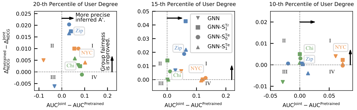
To answer RQ2 and RQ3, we study the relationship between the group fairness and the quality of inferred $A^{\prime}$ . Recall that in Table 3, 4, and 5, the Joint method has smaller $\Delta_{\text{NDCG}}$ than Pre-trained in most cases. To understand the advantage of Joint, Fig. 3 shows the AUC gap of $A^{\prime}$ given by $g_{\bt}$ ( $x$ -axis) in these two settings with corresponding $\Delta_{\text{NDCG}}$ difference ( $y$ -axis). Most models in the area I indicate that Joint simultaneously promotes the accuracy of $g_{\bt}$ and the fairness of $f_{\bw}$ . Since Joint updates $\bt$ using the gradient from $f_{\boldsymbol{W}}$ (see Eq. (LABEL:eq:_update_theta)), our mixup strategies can mitigate the overfitting for $g_{\boldsymbol{\theta}}$ with more gradients from the synthetic data.

3.2.3. Impact of the accurate $A^{\prime}$ on group fairness.

Since the quality of $A^{\prime}$ correlates with the group fairness, we further increase (i.e., Random method) or decrease (i.e., GT method) the noise in $A^{\prime}$ to see if this correlation holds to answer RQ4. Fig. 6 gives $\Delta_{\text{NDCG}}$ for detectors with different ways to assign value to $A^{\prime}$ which contain less and less noise moving from left to right in $x$ -axis. $\Delta_{\text{NDCG}}$ reduces as a detector receives a more accurate inference of the values of $A^{\prime}$ .

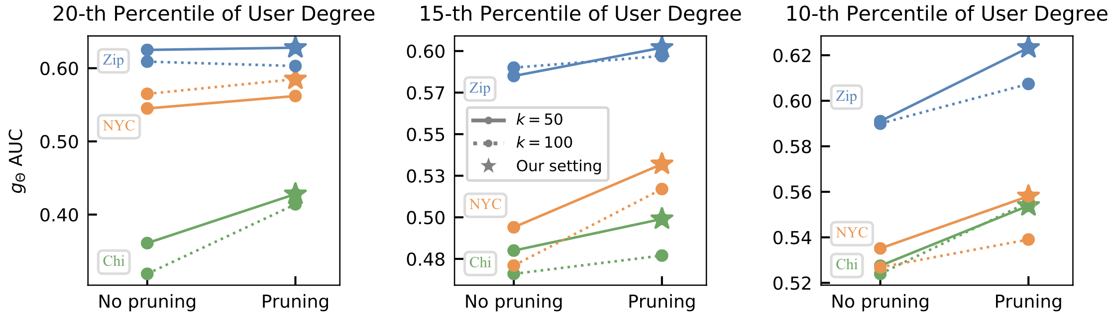
3.3. Sensitivity studies for the replication times $k$ and if pruning non-spam edges.

Fig. 4 shows the test AUCs of $g_{\boldsymbol{\theta}}$ with replications $k=\{50,100\}$ and if pruning non-spams (see Section LABEL:sec:minor_user_augmentation). Pruning has better AUCs than No pruning except when $k=100$ on Zip. Additionally, AUCs for Chi and Zip decrease as increasing the number of $k$ . Since Chi and Zip have few mixed users, forcing the synthesized data to mimic the original node distribution is complex and easy to cause $g_{\bt}$ overfitting. Based on the validation set, we get the optimal $k=100$ for NYC and $k=50$ for Chi and Zip.

Acknowledgements.

To Robert, for the bagels and explaining CMYK and color spaces.

The Name of the Title is Hope

Abstract.

1. Introduction

2. Preliminaries

2.1. Spam detection based on GNN

2.2. Fairness regularizer

3. EXPERIMENTS

3.1. Experimental Settings

3.2. Results

3.2.1. Group Fairness.

3.2.2. Evaluation of the Joint method on improving the quality of A′A^{\prime}.

3.2.3. Impact of the accurate A′A^{\prime} on group fairness.

3.3. Sensitivity studies for the replication times kk and if pruning non-spam edges.

Acknowledgements.

3.2.2. Evaluation of the Joint method on improving the quality of $A^{\prime}$ .

3.2.3. Impact of the accurate $A^{\prime}$ on group fairness.

3.3. Sensitivity studies for the replication times $k$ and if pruning non-spam edges.