The Most Metal-poor Stars in Omega Centauri (NGC 5139)111This paper includes data gathered with the 6.5 meter Magellan Telescopes located at Las Campanas Observatory, Chile.
Abstract
The most massive and complex globular clusters in the Galaxy are thought to have originated as the nuclear cores of now tidally disrupted dwarf galaxies, but the connection between globular clusters and dwarf galaxies is tenuous with the M54/Sagittarius system representing the only unambiguous link. The globular cluster Omega Centauri ( Cen) is more massive and chemically diverse than M 54, and is thought to have been the nuclear star cluster of either the Sequoia or Gaia-Enceladus galaxy. Local Group dwarf galaxies with masses equivalent to these systems often host significant populations of very metal-poor stars ([Fe/H] 2.5), and one might expect to find such objects in Cen. Using high resolution spectra from Magellan-M2FS, we detected 11 stars in a targeted sample of 395 that have [Fe/H] ranging from 2.30 to 2.52. These are the most metal-poor stars discovered in the cluster, and are 5 more metal-poor than Cen’s dominant population. However, these stars are not so metal-poor as to be unambiguously linked to a dwarf galaxy origin. The cluster’s metal-poor tail appears to contain two populations near [Fe/H] 2.1 and 2.4, which are very centrally concentrated but do not exhibit any peculiar kinematic signatures. Several possible origins for these stars are discussed.
1 Introduction
Omega Centauri ( Cen) possesses an elegant complexity that is unmatched by any other Galactic globular cluster. While most globular clusters exhibit metallicity dispersions of 0.05 dex or less (e.g., Carretta et al., 2009; Bailin, 2019), stars in Cen span at least a factor of 100 in [Fe/H]222[A/B] log(NA/NB)star log(NA/NB)☉ for elements A and B. and are distributed into at least 5 distinct populations with unique metallicities (e.g., Suntzeff & Kraft, 1996; Norris & Da Costa, 1995; Norris et al., 1996; Villanova et al., 2007; Johnson & Pilachowski, 2010; Marino et al., 2011; Pancino et al., 2011b). Each distinct metallicity group can be further partitioned into at least 2-3 sub-populations with variable light element chemistry, and Cen may host as many as 15 unique stellar populations (Bellini et al., 2017).
The origin and enrichment history of Cen is currently an open question, but several lines of evidence suggest that the cluster may be the remnant core of a now disrupted dwarf galaxy. For example, Cen is the brightest and most massive globular cluster in the Milky Way, but has a strong retrograde orbit (Dinescu et al., 1999) that may be associated with the capture and disruption of the “Sequoia” galaxy discussed in Myeong et al. (2019). Alternatively, Cen could have once been the nuclear star cluster of the more massive Gaia-Enceladus galaxy (Massari et al., 2019). Bekki & Freeman (2003) used dynamical models to show that a compact nuclear core like Cen could survive such a disruption event, and in fact the long tidal stream recently found by Ibata et al. (2019), which stretches several degrees along the cluster’s orbit, seems to support an accretion origin (see also Simpson et al., 2019). We also note that Cen shares many physical and chemical characteristics with M 54 (e.g., Carretta et al., 2010a), which is the most massive cluster in the Sagittarius dwarf galaxy that is currently being tidally destroyed by the Milky Way.
In terms of size and luminosity, Cen and M 54 lie at the intersection between globular clusters, nuclear star clusters, and Ultra Compact Dwarfs (e.g., Mackey & van den Bergh, 2005; Georgiev et al., 2009; Tolstoy et al., 2009), and may be prototypes for “iron-complex” clusters333Note that iron-complex clusters are generally the same as the “anomalous” and “Type II” clusters identified by Marino et al. (2015) and Milone et al. (2017), respectively. that host multiple generations of stars with different light and heavy element abundances (e.g., Yong et al., 2014; Johnson et al., 2015a; Marino et al., 2015; Da Costa, 2016; Milone et al., 2017). Although a definitive connection between iron-complex clusters and dwarf galaxy nuclei has not yet been established (e.g., see Da Costa, 2016), one possible investigation path is to search for cluster members that may have originally been part of the progenitor galaxy’s field star population. Such stars could be identified as having chemistry that is inconsistent with known globular cluster patterns.
For Cen, the two most likely populations to have originated as dwarf galaxy field stars are those at the highest ([Fe/H] 1) and lowest ([Fe/H] 2) metallicities. On the high metallicity end, stars exhibit relatively small light element abundance variations and critically show an O-Na correlation rather than the expected anti-correlation (Johnson & Pilachowski, 2010; Marino et al., 2011; Pancino et al., 2011a). However, several authors have noted that this particular pattern may be attributed to self-enrichment driven by an unusually long star formation history (Johnson & Pilachowski, 2010; D’Antona et al., 2011; Marino et al., 2011). The iron-complex clusters M 2 (Yong et al., 2014) and NGC 6273 (Johnson et al., 2015a, 2017) also contain minority populations of metal-rich stars with small star-to-star abundance variations, but in these cases no clear O-Na correlations are present. For all three clusters the origins of their metal-rich populations remain ambiguous, and it is not yet possible to differentiate whether these stars were captured from a progenitor galaxy or simply trace prolonged chemical enrichment.
The most metal-poor Cen stars have a greater potential to unambiguously link the cluster with a dwarf galaxy formation environment. For example, Milky Way and extragalactic globular cluster systems exhibit a clear metallicity floor of [Fe/H] 2.3 to 2.5 (e.g., Beasley et al., 2019), which suggests that any Cen stars more metal-poor than this limit likely did not originate in the cluster. The metallicity distribution function of the Sequoia galaxy, proposed by Myeong et al. (2019) as the progenitor system for Cen, is not currently well-constrained, but several estimates indicate that it likely had a mass in excess of 107 M⊙ (e.g., Bekki & Tsujimoto, 2019; Myeong et al., 2019). The dwarf galaxy mass-metallicity relation from Kirby et al. (2013) suggests that such a system should have a mean [Fe/H] 1.5, but if Cen formed in a 1010 M⊙ system, such as Gaia-Enceladus (Helmi et al., 2018), then the host galaxy’s mean metallicity may have been closer to [Fe/H] 0.5. In either case, the metallicity distribution functions of most existing dwarf galaxies exhibit long metal-poor tails that reach at least 1-2 dex lower than their mean [Fe/H] values (e.g., Starkenburg et al., 2010; Kirby et al., 2011; Leaman et al., 2013), which suggests that any dwarf galaxy massive enough to host Cen likely had 1-10 of its stars with [Fe/H] 2.5.
Previous analyses of Cen’s red giant branch (RGB) and subgiant branch (SGB) populations have so far failed to find any stars with [Fe/H] 2.25, which is still within the metallicity realm of Galactic globular clusters. Recent RR Lyrae investigations by Bono et al. (2019) and Magurno et al. (2019) found a small number of stars with [Fe/H] 2.5; however, the mean cluster metallicities of these studies are 0.2-0.3 dex lower than spectroscopic analyses of RGB stars (e.g., Johnson & Pilachowski, 2010), which suggests their true metallicity floor may be closer to [Fe/H] 2.3.
Broad-band color-magnitude diagram analyses alone are unlikely to find very low metallicity stars in Cen because the RGB evolutionary sequences of old populations become difficult to distinguish in color below [Fe/H] 2 (e.g., see Figure 7 of Simpson, 2018). Furthermore, the isochrones of very metal-poor RGB stars in Cen may overlap in color and magnitude space with asymptotic giant branch (AGB) sequences as well. Many of the bluer Cen stars, especially in regions where RGB and AGB stars of different metallicity can mix, do not yet have spectroscopic [Fe/H] determinations, and as a result the most metal-poor stars in the cluster may have been missed by previous surveys. Therefore, we derive spectroscopic [Fe/H] measurements for 395 of the bluest RGB stars in Cen to search for the cluster’s most metal-poor constituents that may link the system to formation in a dwarf galaxy environment.
2 Observations and Data Reduction
All spectroscopic data for this project were obtained using the Michigan-Magellan Fiber System (M2FS; Mateo et al., 2012) and MSpec spectrograph mounted on the Magellan-Clay 6.5m telescope at Las Campanas Observatory. The spectra were acquired in three runs via the M2FS queue that spanned 2015 February 19, 21, 22, 23, and 25 for the first set, 2015 March 01, 02, and 04 for the second set, and 2015 July 18 and 20 for the third set. Ten different fiber configurations were used for seven unique pointings, which are illustrated in the right panel of Figure 1. Three of the fields that overlapped with the cluster core included two separate fiber configurations in order to maximize the number of observed stars. The remaining 4 fields each only included a single fiber configuration.
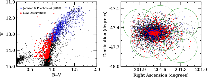
Target stars were selected using the photometry and coordinates from van Leeuwen et al. (2000). Only objects identified by van Leeuwen et al. (2000) as having membership probabilities 70 were targeted, and we prioritized stars on the blue half of the RGB with V magnitudes between about 13.5 and 14.5 (see Figure 1). Although most stars in our sample are first ascent RGB stars, we also included some AGB and red horizontal branch (HB) stars since the isochrones for very metal-poor RGB stars are difficult to distinguish from these later evolutionary stages in more metal-rich populations. Including all configurations, fibers were placed on 458 unique targets spanning a variety of cluster radii (see Figure 1; Table 1); however, we were only able to measure [Fe/H] values for 395 targets. The remaining 63 targets had poor S/N spectra, were heavily blended spectroscopic binaries, or were cases in which we could not converge to a stable model atmosphere solution.
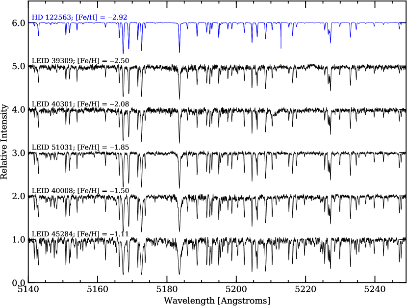
All observations utilized the “MgWide” filters that permit continuous wavelength coverage from approximately 5125-5410 Å. This particular setup was chosen because we are searching for stars with [Fe/H] 2.3 and the Fe lines in this region remain detectable in the spectra of Teff 5000 K RGB stars down to at least [Fe/H] = 4 (e.g., see Figure 1 of Frebel et al., 2015). The “red” and “blue” spectrographs employed identical configurations with 1 2 (dispersion spatial) CCD binning, 95m slits, a four amplifier slow readout, and provided a resolving power of R / 32,000. Since the MgWide filter spans four consecutive orders, we were only able to observe a maximum of 24 targets per spectrograph at a time. Each fiber configuration was observed for one hour with a set of 31200 second exposures.
The data reduction procedure generally followed the methods outlined in Johnson et al. (2015b). Briefly, the IRAF444IRAF is distributed by the National Optical Astronomy Observatory, which is operated by the Association of Universities for Research in Astronomy, Inc., under cooperative agreement with the National Science Foundation. CCDPROC routine was used to apply the bias corrections, trim the overscan regions, and subtract dark current for each amplifier image. The IMTRANSPOSE and IMJOIN routines were then used to align and combine the four amplifier images of every exposure to create sets of monolithic 2K4K images. The DOHYDRA task was utilized to handle aperture identification, aperture tracing, flat-fielding, wavelength calibration via ThAr comparison spectra, scattered light and cosmic ray removal, throughput corrections, and spectrum extraction. Median sky spectra were generated for each order on each night from the designated sky fiber data, and were subtracted from the appropriate science spectra. The sky subtracted data were then corrected for heliocentric velocity variations, continuum normalized, and median combined. Sample combined spectra for several stars with different [Fe/H] but similar temperature and surface gravity values are provided in Figure 2. Signal-to-noise (S/N) ratios for the combined spectra ranged from 20-50 per reduced pixel.
3 Data Analysis
3.1 Model Atmospheres
For consistency with the Johnson & Pilachowski (2010) temperature/gravity scale, model atmosphere parameters were determined for each star using dereddened B, V, and KS-band photometry from van Leeuwen et al. (2000) and the Two Micron All Sky Survey (2MASS; Skrutskie et al., 2006). Although several authors note the existence of minor ( 0.02 mag.) differential reddening near the cluster core (e.g., Calamida et al., 2005; van Loon et al., 2007; McDonald et al., 2009), we assumed a constant E(BV) = 0.11 (Calamida et al., 2005) across the cluster and also utilized the relation E(VKS)/E(BV) = 2.70 from McCall (2004). For target stars with clear 2MASS matches, effective temperatures (Teff) were determined using the VKTCS color-temperature relation from Alonso et al. (1999)555Note that the 2MASS KS-band photometry were transformed onto the KTCS system using the transformations listed in Johnson et al. (2005).. In the few cases where clear 2MASS matches could not be obtained we used the BV color-temperature relation from Alonso et al. (1999) to derive Teff values. The estimated Teff uncertainty is approximately 30 K for temperatures derived from VKTCS and 130 K for BV, based on the scatter of the empirical color-temperature relations in Alonso et al. (1999, see their Table 2).
Similar to Teff, surface gravity (log g) values were determined for each star using photometric temperatures and absolute bolometric magnitudes (Mbol.). The bolometric magnitude values were calculated using the corrections provided by Alonso et al. (1999) and a distance modulus of (mM)V = 13.7 (van de Ven et al., 2006). Final surface gravity values were determined using the relation,
| (1) | |||
where we assumed a mass of 0.8 M⊙ for all stars. Although a mass of 0.8 M⊙ is a reasonable assumption for most cluster RGB stars, Figure 1 shows that some of our targets may be lower mass AGB or red HB stars. McDonald et al. (2011) showed that Cen RGB stars lose 25 of their mass between the RGB and AGB sequences so a significant fraction of our targets may have masses closer to 0.6 M⊙. Fortunately, the photometric surface gravity estimate shown above is only sensitive to the log of the mass difference, and we have restricted the present analysis to only include Fe I lines, which are not strongly pressure sensitive in the stars targeted here. Assuming the difference between RGB and AGB masses does not exceed 0.2 M⊙, we adopt a log(g) uncertainty of 0.15 (cgs).
For most stars in our analysis, the available Fe I lines are too strong to tightly constrain the microturbulence (mic.). Therefore, we determined an empirical relation between Teff and mic. as,
| (2) |
using data from Johnson & Pilachowski (2010) that spanned the same Teff range as the stars presented here. The adopted microturbulence calibration has a dispersion of 0.17 km s-1.
Since the photometric color-temperature relation is dependent on metallicity and the surface gravity and microturbulence estimates require accurate temperature measurements, generating a global model atmosphere solution for each star is an iterative process. Therefore, we initially determined Teff, log(g), and mic. for each star assuming [Fe/H] = 1.7, and iteratively solved for all four parameters as the metallicity determination improved (see also 3.3). We interpolated within the ATLAS9 grid of model atmospheres from Castelli & Kurucz (2003), and in general a stable solution was reached after 3 iterations. The adopted model atmosphere parameters, [Fe/H] values, photometry, star identifiers, and coordinates are provided in Table 1.
3.2 Membership and Radial Velocities
Although cluster membership probabilities were provided by van Leeuwen et al. (2000) based on proper motion measurements, we verified membership using radial velocity measurements as well. Radial velocities were determined using the first exposure of each configuration and comparing it with a synthetic reference spectrum at rest velocity that matched the resolution and sampling of the data. The observed radial velocity values were determined using the XCSAO routine from Kurtz & Mink (1998), and heliocentric corrections were calculated using IRAF’s rvcor routine. The final heliocentric radial velocities and XCSAO error measurements for each star are provided in Table 1.
We found a mean heliocentric radial velocity of 232.5 km s-1 for Cen with a dispersion of 12.8 km s-1. These values are in good agreement with previous work (e.g., Reijns et al., 2006; Sollima et al., 2009). A direct comparison of stars in common between this work and Reijns et al. (2006) gives a mean velocity difference, in the sense of the present work minus the literature, of 1.0 km s-1 with a dispersion of 1.7 km s-1 (55 stars). A similar comparison with Sollima et al. (2009) gives a mean difference of 2.2 km s-1 and a dispersion of 2.9 km s-1 (215 stars). The data presented in Table 1 indicate a radial velocity range spanning 186.7 to 271.1 km s-1; however, given the cluster’s high radial velocity relative to the background and its large velocity dispersion, we designate all stars in our sample as cluster members666We reiterate that the targets have already been selected to have membership probabilities 70, based on the van Leeuwen et al. (2000) proper motion analysis..
3.3 [Fe/H] Determinations
Given the modest S/N ratios of the spectra and the small number of available Fe II lines, all iron abundance determinations were made using synthetic spectrum fits to Fe I features. We first selected a subset of 14 Fe I lines between 5140 and 5390 Å that were visible in a majority of our spectra but had typical equivalent widths lower than about 150 mÅ. The spectrum synthesis line lists were augmented to include significant lines within 5 Å of each Fe I feature listed in Table 2. Due to a paucity of high accuracy experimental log gf values for the features given in Table 2, empirical log gf values were determined for all lines by first adopting atomic data from the Vienna Atomic Line Database (Ryabchikova et al., 2015) compilation and then adjusting the log gf values until a satisfactory fit to an M2FS daylight solar spectrum was achieved. We adopted the Anders & Grevesse (1989) solar abundances for all elements777Note that the Anders & Grevesse (1989) solar abundances were used for consistency with Johnson & Pilachowski (2010).. Although MgH lines may be present at wavelengths bluer than 5200 Å, the roughly 4800 K temperatures and low metallicities of our stars inhibited significant molecular contamination. Furthermore, we only selected Fe I lines that were at least 0.5 Å away from significant molecular blends. As a result, the adopted line list only included atomic features. The adopted atomic parameters for all Fe I lines of interest are provided in Table 2.
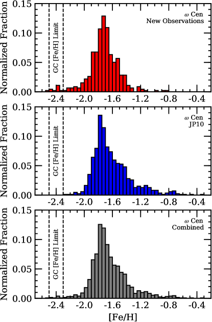
As mentioned previously, an initial estimate of Teff, log(g), and mic. was made for each star assuming [Fe/H] = 1.7. For the first iteration, the Teff, log(g), and mic. values were held fixed while model atmospheres and synthetic spectra were generated for [Fe/H] values ranging from 2.75 to 0.5, in 0.01 dex steps, using the LTE line analysis code MOOG (Sneden, 1973). The fits for each line were visually inspected to identify and remove lines affected by spectrum flaws, to set appropriate smoothing/broadening parameters, and to remove extreme outliers ( 0.3 dex from the mean). The [Fe/H] abundance that minimized the fitting residuals between the synthetic and observed spectra was selected as the new metallicity parameter, which enabled an update to the Teff, log(g), and mic. values. This process was repeated until the difference in mean [Fe/H] between consecutive runs decreased to 0.03 dex, and then a final iteration was performed. The adopted [Fe/H] abundances for each star are provided in Table 1 and also summarized as a histogram in Figure 3.
The targets were selected to have minimal overlap with other high resolution spectroscopic studies; however, the present sample does have 8 stars in common with Marino et al. (2011). A comparison between the two studies indicates good agreement with a mean offset in [Fe/H] of 0.0 dex and a dispersion of 0.13 dex, which is comparable to the mean line-to-line [Fe/H] dispersion reported in Table 1 for our analysis. We also have 52 stars in common with the low resolution (R 2000) spectroscopic analysis by An et al. (2017) that shows a mean offset, in the sense of the present work minus the literature value, of 0.12 dex and a dispersion of 0.15 dex. We attribute the worse agreement to the order of magnitude lower resolution in the An et al. (2017) data.
The [Fe/H] error values ([Fe/H]) provided in Table 1 take into account several factors added in quadrature, including the standard error of the mean [Fe/H] value and uncertainties related to temperature (Teff = 100 K), surface gravity (log(g) = 0.15 cgs), model atmosphere metallicity ([M/H] = 0.15 dex), and microturbulence (mic. = 0.13 km s-1) errors. However, since we exclusively used Fe I lines the error budget is dominated by the Teff, mic., and measurement uncertainties, which also includes log gf and continuum normalization and/or fitting errors. Typical uncertainties are approximately 0.14 dex in [Fe/H]. Since corrections for departures from local thermodynamic equilibrium (LTE) are not available for several of the lines used here, all [Fe/H] measurements assume LTE. Fortunately, calculations from several authors (Bergemann et al., 2012; Lind et al., 2012; Mashonkina et al., 2016) indicate that absolute Fe I non-LTE corrections should be 0.05-0.10 dex in magnitude for the parameter space analyzed here. Relative differences between stars with similar temperatures should be even smaller.
4 Results and Discussion
As mentioned in 1, one of Cen’s most intriguing properties is its large metallicity spread. Numerous authors have used large sample spectroscopic (Norris & Da Costa, 1995; Norris et al., 1996; Suntzeff & Kraft, 1996; Villanova et al., 2007; Johnson et al., 2008; Johnson & Pilachowski, 2010; Marino et al., 2011; Pancino et al., 2011b, a; Villanova et al., 2014; An et al., 2017; Mucciarelli et al., 2018) and photometric (Lee et al., 1999; Hilker & Richtler, 2000; Pancino et al., 2000; Rey et al., 2004; Sollima et al., 2005; Calamida et al., 2009; Bellini et al., 2010; Calamida et al., 2017) surveys to show that the cluster has at least 5-6 populations with unique [Fe/H] values. Peaks in the metallicity distribution function are generally found near [Fe/H] 1.75, 1.50, 1.20, and 0.70 (see also Figure 3), and tend to cluster on well-defined RGB sequences. Pancino et al. (2011b) claim to find a more metal-poor population, rather than simply a metal-poor tail, near [Fe/H] 2, which suggests that additional minority populations of very metal-poor stars may still be awaiting discovery.
Finding cluster members with [Fe/H] 2.3 would be important for linking Cen’s formation to a dwarf galaxy environment because such stars are not expected in globular clusters. A nearly universal globular cluster metallicity floor exists near [Fe/H] 2.3 to 2.5 for Local Group galaxies (e.g., Beasley et al., 2019) as well as the Milky Way (e.g., Simpson, 2018), and Cen’s retrograde, but confined to the plane (e.g., Majewski et al., 2012), orbit precludes capturing metal-poor stars from the Galactic halo. Therefore, very metal-poor stars found in Cen today would likely have originated as a field population in the cluster’s progenitor system. If Cen formed in an environment similar to the dwarf galaxies observed today, then knowledge of the cluster’s [Fe/H] floor could help place constraints on the metallicity distribution function of its host galaxy.
4.1 Very Metal-poor Stars in Cen
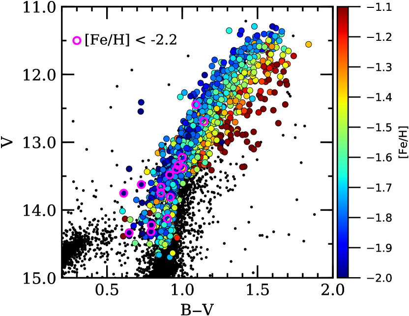
In Figure 3 we compare the biased metallicity distribution function derived here against the relatively unbiased distribution found by Johnson & Pilachowski (2010). The new observations clearly confirm the presence of the dominant metal-poor population near [Fe/H] 1.7 and the intermediate metallicity group at [Fe/H] 1.5, and as expected from our selection procedure we find far fewer stars with [Fe/H] 1.3. Figure 4 further shows that our [Fe/H] determinations follow the expected correlation between metallicity and RGB color, and that most of the stars in our sample with [Fe/H] 1.3 lie on the AGB or red HB sequences.
We find a possible metal-poor population near [Fe/H] 2.1 that appears separate from the dominant group at [Fe/H] 1.7 (see also 4.1.1), and we suspect that these RGB stars are part of the same metal-poor faction identified by Pancino et al. (2011b) on the SGB. Interestingly, we also find a new population of 11 stars with metallicities below the [Fe/H] = 2.26 limit set by Johnson & Pilachowski (2010). These stars represent 2.8 of our sample and span from [Fe/H] = 2.30 to 2.52. Figure 4 further shows that these very metal-poor stars generally fall on the blue edge of the cluster RGB, as expected, but 2-3 of the targets could be AGB or HB stars. The very metal-poor stars identified here are close to the empirically determined globular cluster metallicity floor noted in Beasley et al. (2019).
The existence of a metal-poor tail in Cen is already a unique trait among iron-complex clusters. The metallicity distribution functions for all iron-complex clusters except Cen possess a sharp rise at low metallicity, one or more populations at higher metallicity, and occasionally a metal-rich tail. The only other compelling case for a cluster hosting a metal-poor tail or a minor population at low metallicity is Terzan 5, which has a dominant population near [Fe/H] 0.3, a secondary population at [Fe/H] 0.25, and a minority ( 6) metal-poor group at [Fe/H] 0.8 (Origlia et al., 2013; Massari et al., 2014). However, the various Terzan 5 sub-populations do not possess the complex light element variations observed in Cen.
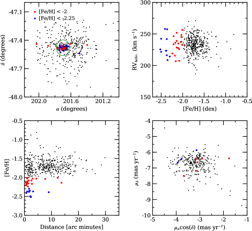
Other than metallicity, do the most metal-poor stars in Cen possess any unusual properties? Figure 5 compares the radial and spatial distributions, radial velocities, and Gaia DR2 proper motions for the stars analyzed in the present study. Visual inspection of the two left panels in Figure 5 indicate that: (1) stars with [Fe/H] 2 span a broad range in right ascension but only populate a narrow range in declination and (2) the most metal-poor stars may be very centrally concentrated. First addressing the spatial distribution, we note that the dispersion in declination for stars with [Fe/H] 2 is 0.128 degrees while the dispersions for stars with 2.25 [Fe/H] 2 and [Fe/H] 2.25 are 0.023 and 0.029 degrees, respectively. Similarly, two-sided Kolmogorov-Smirnov (KS) tests comparing the declination distributions of all stars versus first those with [Fe/H] 2 and then those with [Fe/H] 2.25 returned -values888We adopt the common convention that a -value 0.05 is sufficient to reject the null hypothesis. of 0.002 and 0.095, respectively. From these data we can conclude that there is marginal evidence indicating that the most metal-poor Cen stars may be confined to a more narrow plane than the majority of cluster stars. However, a larger sample size is required to draw any strong conclusions.
Regarding the radial distributions, Figure 5 shows that nearly all of the stars with [Fe/H] 2 are projected within 12 of the cluster core and 84 are within 3. Similarly, all of the stars with [Fe/H] 2.25 are within 10 and 81 are inside of 3. These results match previous observations by Johnson & Pilachowski (2010) who noted that 88 of the stars in their sample with [Fe/H] 2 were found within 5 of the cluster core. The combination of the present work with the larger sample of Johnson & Pilachowski (2010) hints that the most metal-poor stars in Cen may be mostly confined to within a half-light radius (5). A two-sided KS test comparing the radial distributions of stars with [Fe/H] 2 against those with [Fe/H] 2 returned a -value of 2.9110-10 while a similar test comparing the radial distributions of stars with [Fe/H] 2 and [Fe/H] 2.25 returned a -value of 8.6610-5. The extremely low -values indicate a low probability that stars with [Fe/H 2 follow the same radial distribution as their higher metallicity counterparts. We did not detect any further differences between the most metal-poor stars and any other populations when examining radial velocity or proper motion distributions; however, larger sample sizes are required to draw any firm conclusions.
4.1.1 Do the Very Metal-poor Stars Form Distinct Populations?
An important question when examining the metallicity distribution function of Cen is whether the stars with [Fe/H] 2 form distinct populations or simply an extended tail. As noted previously, the binned distributions shown in Figure 3 indicate possible “peaks” near [Fe/H] 2.1 and 2.4, but the sample sizes are small. To help determine whether the most metal-poor stars are separate populations, we utilize the Gaussian mixture model (GMM) method described in Ashman et al. (1994) via the implementation outlined in Muratov & Gnedin (2010) to examine: (1) if the peak near [Fe/H] = 2.1 is distinct from the dominant population near [Fe/H] = 1.7; and (2) if the groups at [Fe/H] = 2.1 and 2.4 are separate or part of a broad unimodal population.
The modality analysis described in Muratov & Gnedin (2010) includes an algorithm for a likelihood ratio test that determines whether the sum of two Gaussian profiles provides an improvement over fitting a unimodal Gaussian distribution. Note that we have adopted the homoschedastic case (equal variance) for all GMM tests, which is a reasonable assumption if the [Fe/H] spread within each population is dominated by equivalent measurement errors. Since the likelihood ratio test assumes Gaussian distributions, Ashman et al. (1994) and Muratov & Gnedin (2010) also include a dimensionless mode separation statistic defined as,
| (3) |
where D 2 is required for a clear separation between two modes when the mean () and dispersion () values for two populations are known. Muratov & Gnedin (2010) also note that a negative kurtosis is a “necessary but not sufficient condition of bimodality”. However, since the number of very metal-poor stars in our sample is small, especially relative to the dominant population at [Fe/H] 1.7, we do not include kurtosis measurements here.
For the first case listed above, we compiled a list of stars with 2.25 [Fe/H] 1.60 from Table 1 and ran the Muratov & Gnedin (2010) algorithm to determine whether a bimodal distribution was an improvement over fitting a single Gaussian profile. The Muratov & Gnedin (2010) test found that the data were better fit assuming two Gaussian distributions with means of [Fe/H] = 2.07 and 1.76 ( = 0.09 dex) over a single Gaussian with a mean of [Fe/H] = 1.78 and a larger dispersion ( = 0.11 dex) at more than the 99.9 level. A bootstrap analysis yielded a separation statistic of D = 3.38 0.41, which provides a high level of confidence that the peak at [Fe/H] = 2.07 represents a legitimate population rather than a metal-poor tail for the [Fe/H] = 1.76 group.
For the second case, we examined the [Fe/H] distribution for all stars in Table 1 with [Fe/H] 2 to determine if these objects form two narrow populations or one broad distribution. We determined that a unimodal distribution was ruled out at the more than 99.6 level, and that two populations were preferred having means of [Fe/H] = 2.4 and 2.1 with dispersions of 0.07 dex. The bootstrap mode separation statistic was calculated to be D = 4.37 0.8, which suggests that if two populations are present below [Fe/H] = 2 then their mean metallicities are well-separated.
4.2 Origin of the Very Metal-poor Stars
If the stars in Cen with [Fe/H] 2, and especially those with [Fe/H] 2.25, are truly distinct from the other cluster populations, then their presence may reveal important details about the cluster’s early formation history. The available evidence suggests several possible origins for Cen’s very metal-poor stars, including: (1) early star formation in the unenriched primordial cloud, (2) the capture of surrounding field stars, assuming the cluster formed in a dwarf galaxy, or (3) an early merger between Cen and a pre-existing but metal-poor sub-structure.
4.2.1 Early Star Formation
The primordial cloud scenario is the most straight-forward, and would imply that the very metal-poor stars trace the original composition of the molecular cloud from which Cen formed. Data from Johnson & Pilachowski (2010) and Pancino et al. (2011b) indicate that stars with [Fe/H] 2 may have reduced light element abundance variations compared to their more metal-rich counterparts, which might be consistent with an early proto-cluster environment that had not yet been polluted by sources such as intermediate mass AGB stars. However, if Cen actually has two populations of very metal-poor stars at [Fe/H] 2.1 and 2.4, as is suggested in Figure 3 and 4.1.1, then the cluster could have experienced at least two early small bursts of star formation. Detailed light and heavy element abundance measurements for the [Fe/H] 2.4 stars identified here would help determine if the two groups are chemically similar.
Examining the published metallicity distribution functions of other iron-complex clusters, we note that aside from Terzan 5 only M 54 appears as a possible candidate to host a metal-poor tail. However, the most metal-poor stars in this system were clearly polluted, as evidenced by their large (anti-)correlated light element abundance variations (e.g., Carretta et al., 2010b), and would therefore not represent a pristine population. Similarly, we note that monometallic clusters have significant populations of “primordial” stars that appear to be almost entirely polluted by supernovae, but these stars do not have different [Fe/H] abundances from other cluster members. Therefore, either Cen and Terzan 5 were unique in their ability to retain stars that formed before the first major star formation and light element enrichment episode, or their very metal-poor populations have a different origin.
4.2.2 Captured Field Stars
The captured field star scenario is intriguing because it could provide a direct link between present day iron-complex clusters and dwarf galaxies. However, if Cen formed within a dwarf galaxy should we expect such a system to host many very metal-poor stars? We can draw two reasonable conclusions based on Cen’s properties alone. First, Cen’s mass of 4106 M☉ (D’Souza & Rix, 2013) means that its host galaxy must have had a mass of at least 107-108 M☉ (see also Bekki & Tsujimoto, 2019; Myeong et al., 2019). Second, the dwarf galaxy mass-metallicity relation from Kirby et al. (2013) implies that the cluster’s host galaxy likely had a mean metallicity of at least [Fe/H] = 1.5 to 1. A comparatively high metallicity field star population is qualitatively in agreement with the M 54/Sagittarius system where the mean metallicity of M 54 ([Fe/H] 1.6) is several times lower than the Sagittarius field (e.g., Carretta et al., 2010b). Nevertheless, dwarf galaxies tend to have long metal-poor tails (e.g., Leaman et al., 2013), and even cases such as Sagittarius that have a majority of stars with [Fe/H] 1 contain stars with metallicities as low as 2.2 (Chiti & Frebel, 2019). It therefore remains plausible that Cen could have existed in an environment that also hosted very metal-poor field stars.
The ability of Cen to capture very metal-poor stars might depend not only on the metallicity distribution of its host galaxy, but also the cluster’s typical galactocentric radius and the galaxy’s star formation history before tidal disruption. Existing Local Group dwarf galaxies generally exhibit negative metallicity gradients such that the mean metallicity decreases at larger galactocentric distances (e.g., Harbeck et al., 2001; Battaglia et al., 2006; Faria et al., 2007; Carrera et al., 2008; Kirby et al., 2011; Kacharov et al., 2017). If Cen resided in the core of its host galaxy and a significant fraction of the cluster’s metal-poor stars were captured, then Cen’s host galaxy might have had an unusually metal-poor core. Alternatively, the cluster’s host galaxy could have had an inverted metallicity gradient (e.g., Wang et al., 2019).
Although Cen is the most massive cluster associated with the Sequoia (Myeong et al., 2019) or Gaia-Enceladus (Massari et al., 2019) merger events, that does not necessarily mean the cluster always (or ever) resided in its host galaxy’s center. For example, M 54 is the most massive cluster associated with Sagittarius and presently lies near the galaxy’s core, but the cluster could have formed outside the galaxy nucleus and drifted to the center via dynamical friction (e.g., Bellazzini et al., 2008). Furthermore, the Fornax dwarf galaxy has five globular clusters (Shapley, 1938; Hodge, 1961) and all except one (Fornax 4), including the most massive and metal-poor cluster Fornax 3 (de Boer & Fraser, 2016), reside well outside the core radius. One might expect that if Cen were in a configuration similar to that of Fornax 3 it would have a reasonable chance of capturing metal-poor field stars.
Regardless of where Cen may have resided within a host galaxy, it could not capture metal-poor field stars unless they were present in significant numbers. Combining the present sample with Johnson & Pilachowski (2010), 3.9 of stars in Cen have [Fe/H] 2 and about 1 have [Fe/H] 2.3. For comparison, Starkenburg et al. (2010) showed that the fractions of stars with [Fe/H] 2.5 were 1, 8, 8, and 33 for the Fornax, Carina, Sculptor, and Sextans Local Group dwarf galaxies, respectively.
These observations suggest that Cen’s host galaxy probably had a higher fraction of metal-poor stars than Fornax, especially if all Cen stars with [Fe/H] 2 were captured. In contrast, the metallicity distribution of Sextans may be too metal-poor since we did not find any stars with [Fe/H] 2.5. However, we investigated the color-color distribution of stars in Cen using recent Sky Mapper (Wolf et al., 2018) photometry and found a small number of stars that may have [Fe/H] 2.5 to 3. A galaxy like Sculptor, but with the globular cluster specific frequency of Fornax, may serve as a reasonable model of Cen’s host galaxy since it has: (1) a mean [Fe/H] value that is higher than Cen, (2) a small but significant population of field stars down to [Fe/H] 3.0, and (3) few stars with [Fe/H] 1 (e.g., Kirby et al., 2009; Starkenburg et al., 2010). The small ( 10 km s-1) velocity dispersion of Fornax globular clusters and field stars (e.g., Hendricks et al., 2014) would also provide a model that is conducive to tidal capture, but it remains to be seen whether such a scenario could be reconciled with the observed central concentration of very metal-poor stars in Cen.
4.2.3 Merging Sub-clumps
Globular clusters are likely the end results of complicated hierarchical merging processes (e.g., Bonnell et al., 2003; Smilgys & Bonnell, 2017), and in this sense the rarity of very metal-poor stars among iron-complex clusters could be a result of this stochastic process. Sub-clump and cluster-cluster mergers have been invoked to explain several globular cluster properties in the past (e.g., van den Bergh, 1996; Lee et al., 1999; Carretta et al., 2010c; Bekki & Tsujimoto, 2019), and we posit that such a model may explain the existence of the metal-poor populations in Cen, and possibly Terzan 5, as well.
In this model, the early Cen environment would have been subject to intense star formation and molecular cloud and/or cluster mergers. As a result, the main Cen structure could have coalesced with a sub-structure that was either in the process of forming or already fully formed, but that had a very low metallicity and not enough time to experience significant light element self-enrichment. Since the most metal-poor stars in Cen do not reach below the empirical globular cluster limit of [Fe/H] 2.5 and Figure 3 hints at two different populations with [Fe/H] 2 rather than a continuous metal-poor tail, a merging sub-structure scenario may be favored over a field star capture model. If the merging sub-structures were also relatively massive, they might naturally fall to the cluster center and help explain the central concentration of stars with [Fe/H] 2 shown in Figure 5.
Although the stars with [Fe/H] 2 constitute only a small fraction of Cen’s mass, we did not detect any unusual kinematic properties for these populations. As a result, the sub-clump merger origin for very metal-poor stars may only be plausible if their initial kinematic signature was erased by dynamical evolution or was very similar to the existing Cen proto-cluster.
5 Summary
We present [Fe/H] measurements, based on high resolution M2FS spectra, for 395 giants in the massive globular cluster Cen. The targets were chosen to reside on the blue half of the RGB in an effort to find the most metal-poor stars in the cluster. Previous attempts identified a metal-poor population with [Fe/H] 2.1 but failed to find any stars with [Fe/H] 2.25. However, we have identified 11 new stars with metallicities ranging from [Fe/H] = 2.30 to 2.52, which places these stars near the empirical globular cluster metallicity floor observed among the Milky Way and other Local Group galaxies.
The metal-poor stars identified here and in previous studies appear to be very centrally concentrated, and may also be confined to a narrow declination plane. However, these stars do not appear to exhibit any peculiar kinematic properties that distinguish them from the more metal-rich populations in Cen. We examine three possible scenarios in which Cen could form or capture stars that are significantly more metal-poor than its dominant population at [Fe/H] 1.7. Specifically, the very metal-poor stars could: (1) trace very early star formation in the cluster, (2) have originated as captured field stars from Cen’s original host galaxy, or (3) represent an early merger event between Cen and metal-poor sub-clumps. Although none of these scenarios is clearly favored, the merging sub-clump model may have the greatest chance for describing the paucity of very metal-poor stars in other clusters, the possibly reduced light element spread for stars with [Fe/H] 2, and the observed central concentration of these populations.
References
- Afsar et al. (2016) Afsar, M., Sneden, C., Frebel, A., et al. 2016, ApJ, 819, 103, doi: 10.3847/0004-637X/819/2/103
- Alonso et al. (1999) Alonso, A., Arribas, S., & Martínez-Roger, C. 1999, A&AS, 140, 261, doi: 10.1051/aas:1999521
- An et al. (2017) An, D., Lee, Y. S., In Jung, J., et al. 2017, AJ, 154, 150, doi: 10.3847/1538-3881/aa8364
- Anders & Grevesse (1989) Anders, E., & Grevesse, N. 1989, Geochim. Cosmochim. Acta, 53, 197, doi: 10.1016/0016-7037(89)90286-X
- Ashman et al. (1994) Ashman, K. M., Bird, C. M., & Zepf, S. E. 1994, AJ, 108, 2348, doi: 10.1086/117248
- Bailin (2019) Bailin, J. 2019, arXiv e-prints, arXiv:1909.11731. https://arxiv.org/abs/1909.11731
- Battaglia et al. (2006) Battaglia, G., Tolstoy, E., Helmi, A., et al. 2006, A&A, 459, 423, doi: 10.1051/0004-6361:20065720
- Beasley et al. (2019) Beasley, M. A., Leaman, R., Gallart, C., et al. 2019, MNRAS, 487, 1986, doi: 10.1093/mnras/stz1349
- Bekki & Freeman (2003) Bekki, K., & Freeman, K. C. 2003, MNRAS, 346, L11, doi: 10.1046/j.1365-2966.2003.07275.x
- Bekki & Tsujimoto (2019) Bekki, K., & Tsujimoto, T. 2019, arXiv e-prints, arXiv:1909.11295. https://arxiv.org/abs/1909.11295
- Bellazzini et al. (2008) Bellazzini, M., Ibata, R. A., Chapman, S. C., et al. 2008, AJ, 136, 1147, doi: 10.1088/0004-6256/136/3/1147
- Bellini et al. (2010) Bellini, A., Bedin, L. R., Piotto, G., et al. 2010, AJ, 140, 631, doi: 10.1088/0004-6256/140/2/631
- Bellini et al. (2017) Bellini, A., Milone, A. P., Anderson, J., et al. 2017, ApJ, 844, 164, doi: 10.3847/1538-4357/aa7b7e
- Bergemann et al. (2012) Bergemann, M., Lind, K., Collet, R., Magic, Z., & Asplund, M. 2012, MNRAS, 427, 27, doi: 10.1111/j.1365-2966.2012.21687.x
- Bonnell et al. (2003) Bonnell, I. A., Bate, M. R., & Vine, S. G. 2003, MNRAS, 343, 413, doi: 10.1046/j.1365-8711.2003.06687.x
- Bono et al. (2019) Bono, G., Iannicola, G., Braga, V. F., et al. 2019, ApJ, 870, 115, doi: 10.3847/1538-4357/aaf23f
- Calamida et al. (2005) Calamida, A., Stetson, P. B., Bono, G., et al. 2005, ApJ, 634, L69, doi: 10.1086/498691
- Calamida et al. (2009) Calamida, A., Bono, G., Stetson, P. B., et al. 2009, ApJ, 706, 1277, doi: 10.1088/0004-637X/706/2/1277
- Calamida et al. (2017) Calamida, A., Strampelli, G., Rest, A., et al. 2017, AJ, 153, 175, doi: 10.3847/1538-3881/aa6397
- Carrera et al. (2008) Carrera, R., Gallart, C., Aparicio, A., et al. 2008, AJ, 136, 1039, doi: 10.1088/0004-6256/136/3/1039
- Carretta et al. (2009) Carretta, E., Bragaglia, A., Gratton, R., D’Orazi, V., & Lucatello, S. 2009, A&A, 508, 695, doi: 10.1051/0004-6361/200913003
- Carretta et al. (2010a) Carretta, E., Bragaglia, A., Gratton, R. G., et al. 2010a, ApJ, 714, L7, doi: 10.1088/2041-8205/714/1/L7
- Carretta et al. (2010b) —. 2010b, A&A, 520, A95, doi: 10.1051/0004-6361/201014924
- Carretta et al. (2010c) Carretta, E., Gratton, R. G., Lucatello, S., et al. 2010c, ApJ, 722, L1, doi: 10.1088/2041-8205/722/1/L1
- Castelli & Kurucz (2003) Castelli, F., & Kurucz, R. L. 2003, in IAU Symposium, Vol. 210, Modelling of Stellar Atmospheres, ed. N. Piskunov, W. W. Weiss, & D. F. Gray, A20. https://arxiv.org/abs/astro-ph/0405087
- Chiti & Frebel (2019) Chiti, A., & Frebel, A. 2019, ApJ, 875, 112, doi: 10.3847/1538-4357/ab0f9f
- Da Costa (2016) Da Costa, G. S. 2016, in IAU Symposium, Vol. 317, The General Assembly of Galaxy Halos: Structure, Origin and Evolution, ed. A. Bragaglia, M. Arnaboldi, M. Rejkuba, & D. Romano, 110–115, doi: 10.1017/S174392131500678X
- D’Antona et al. (2011) D’Antona, F., D’Ercole, A., Marino, A. F., et al. 2011, ApJ, 736, 5, doi: 10.1088/0004-637X/736/1/5
- de Boer & Fraser (2016) de Boer, T. J. L., & Fraser, M. 2016, A&A, 590, A35, doi: 10.1051/0004-6361/201527580
- Dinescu et al. (1999) Dinescu, D. I., Girard, T. M., & van Altena, W. F. 1999, AJ, 117, 1792, doi: 10.1086/300807
- D’Souza & Rix (2013) D’Souza, R., & Rix, H.-W. 2013, MNRAS, 429, 1887, doi: 10.1093/mnras/sts426
- Faria et al. (2007) Faria, D., Feltzing, S., Lundström, I., et al. 2007, A&A, 465, 357, doi: 10.1051/0004-6361:20065244
- Frebel et al. (2015) Frebel, A., Chiti, A., Ji, A. P., Jacobson, H. R., & Placco, V. M. 2015, ApJ, 810, L27, doi: 10.1088/2041-8205/810/2/L27
- Georgiev et al. (2009) Georgiev, I. Y., Hilker, M., Puzia, T. H., Goudfrooij, P., & Baumgardt, H. 2009, MNRAS, 396, 1075, doi: 10.1111/j.1365-2966.2009.14776.x
- Harbeck et al. (2001) Harbeck, D., Grebel, E. K., Holtzman, J., et al. 2001, AJ, 122, 3092, doi: 10.1086/324232
- Helmi et al. (2018) Helmi, A., Babusiaux, C., Koppelman, H. H., et al. 2018, Nature, 563, 85, doi: 10.1038/s41586-018-0625-x
- Hendricks et al. (2014) Hendricks, B., Koch, A., Walker, M., et al. 2014, A&A, 572, A82, doi: 10.1051/0004-6361/201424645
- Hilker & Richtler (2000) Hilker, M., & Richtler, T. 2000, A&A, 362, 895. https://arxiv.org/abs/astro-ph/0008500
- Hodge (1961) Hodge, P. W. 1961, AJ, 66, 83, doi: 10.1086/108378
- Ibata et al. (2019) Ibata, R. A., Bellazzini, M., Malhan, K., Martin, N., & Bianchini, P. 2019, Nature Astronomy, 3, 667, doi: 10.1038/s41550-019-0751-x
- Johnson et al. (2017) Johnson, C. I., Caldwell, N., Rich, R. M., et al. 2017, ApJ, 836, 168, doi: 10.3847/1538-4357/836/2/168
- Johnson et al. (2005) Johnson, C. I., Kraft, R. P., Pilachowski, C. A., et al. 2005, PASP, 117, 1308, doi: 10.1086/497435
- Johnson & Pilachowski (2010) Johnson, C. I., & Pilachowski, C. A. 2010, ApJ, 722, 1373, doi: 10.1088/0004-637X/722/2/1373
- Johnson et al. (2008) Johnson, C. I., Pilachowski, C. A., Simmerer, J., & Schwenk, D. 2008, ApJ, 681, 1505, doi: 10.1086/588634
- Johnson et al. (2015a) Johnson, C. I., Rich, R. M., Pilachowski, C. A., et al. 2015a, AJ, 150, 63, doi: 10.1088/0004-6256/150/2/63
- Johnson et al. (2015b) Johnson, C. I., McDonald, I., Pilachowski, C. A., et al. 2015b, AJ, 149, 71, doi: 10.1088/0004-6256/149/2/71
- Kacharov et al. (2017) Kacharov, N., Battaglia, G., Rejkuba, M., et al. 2017, MNRAS, 466, 2006, doi: 10.1093/mnras/stw3188
- Kirby et al. (2013) Kirby, E. N., Cohen, J. G., Guhathakurta, P., et al. 2013, ApJ, 779, 102, doi: 10.1088/0004-637X/779/2/102
- Kirby et al. (2009) Kirby, E. N., Guhathakurta, P., Bolte, M., Sneden, C., & Geha, M. C. 2009, ApJ, 705, 328, doi: 10.1088/0004-637X/705/1/328
- Kirby et al. (2011) Kirby, E. N., Lanfranchi, G. A., Simon, J. D., Cohen, J. G., & Guhathakurta, P. 2011, ApJ, 727, 78, doi: 10.1088/0004-637X/727/2/78
- Kurtz & Mink (1998) Kurtz, M. J., & Mink, D. J. 1998, PASP, 110, 934, doi: 10.1086/316207
- Leaman et al. (2013) Leaman, R., Venn, K. A., Brooks, A. M., et al. 2013, ApJ, 767, 131, doi: 10.1088/0004-637X/767/2/131
- Lee et al. (1999) Lee, Y. W., Joo, J. M., Sohn, Y. J., et al. 1999, Nature, 402, 55, doi: 10.1038/46985
- Lind et al. (2012) Lind, K., Bergemann, M., & Asplund, M. 2012, MNRAS, 427, 50, doi: 10.1111/j.1365-2966.2012.21686.x
- Mackey & van den Bergh (2005) Mackey, A. D., & van den Bergh, S. 2005, MNRAS, 360, 631, doi: 10.1111/j.1365-2966.2005.09080.x
- Magurno et al. (2019) Magurno, D., Sneden, C., Bono, G., et al. 2019, ApJ, 881, 104, doi: 10.3847/1538-4357/ab2e76
- Majewski et al. (2012) Majewski, S. R., Nidever, D. L., Smith, V. V., et al. 2012, ApJ, 747, L37, doi: 10.1088/2041-8205/747/2/L37
- Marino et al. (2011) Marino, A. F., Milone, A. P., Piotto, G., et al. 2011, ApJ, 731, 64, doi: 10.1088/0004-637X/731/1/64
- Marino et al. (2015) Marino, A. F., Milone, A. P., Karakas, A. I., et al. 2015, MNRAS, 450, 815, doi: 10.1093/mnras/stv420
- Mashonkina et al. (2016) Mashonkina, L. I., Sitnova, T. N., & Pakhomov, Y. V. 2016, Astronomy Letters, 42, 606, doi: 10.1134/S1063773716080028
- Massari et al. (2019) Massari, D., Koppelman, H. H., & Helmi, A. 2019, A&A, 630, L4, doi: 10.1051/0004-6361/201936135
- Massari et al. (2014) Massari, D., Mucciarelli, A., Ferraro, F. R., et al. 2014, ApJ, 795, 22, doi: 10.1088/0004-637X/795/1/22
- Mateo et al. (2012) Mateo, M., Bailey, J. I., Crane, J., et al. 2012, in Society of Photo-Optical Instrumentation Engineers (SPIE) Conference Series, Vol. 8446, Proc. SPIE, 84464Y, doi: 10.1117/12.926448
- McCall (2004) McCall, M. L. 2004, AJ, 128, 2144, doi: 10.1086/424933
- McDonald et al. (2011) McDonald, I., Johnson, C. I., & Zijlstra, A. A. 2011, MNRAS, 416, L6, doi: 10.1111/j.1745-3933.2011.01086.x
- McDonald et al. (2009) McDonald, I., van Loon, J. T., Decin, L., et al. 2009, MNRAS, 394, 831, doi: 10.1111/j.1365-2966.2008.14370.x
- Milone et al. (2017) Milone, A. P., Piotto, G., Renzini, A., et al. 2017, MNRAS, 464, 3636, doi: 10.1093/mnras/stw2531
- Mucciarelli et al. (2018) Mucciarelli, A., Salaris, M., Monaco, L., et al. 2018, A&A, 618, A134, doi: 10.1051/0004-6361/201833457
- Muratov & Gnedin (2010) Muratov, A. L., & Gnedin, O. Y. 2010, ApJ, 718, 1266, doi: 10.1088/0004-637X/718/2/1266
- Myeong et al. (2019) Myeong, G. C., Vasiliev, E., Iorio, G., Evans, N. W., & Belokurov, V. 2019, MNRAS, 488, 1235, doi: 10.1093/mnras/stz1770
- Norris & Da Costa (1995) Norris, J. E., & Da Costa, G. S. 1995, ApJ, 447, 680, doi: 10.1086/175909
- Norris et al. (1996) Norris, J. E., Freeman, K. C., & Mighell, K. J. 1996, ApJ, 462, 241, doi: 10.1086/177145
- Origlia et al. (2013) Origlia, L., Massari, D., Rich, R. M., et al. 2013, ApJ, 779, L5, doi: 10.1088/2041-8205/779/1/L5
- Pancino et al. (2000) Pancino, E., Ferraro, F. R., Bellazzini, M., Piotto, G., & Zoccali, M. 2000, ApJ, 534, L83, doi: 10.1086/312658
- Pancino et al. (2011a) Pancino, E., Mucciarelli, A., Bonifacio, P., Monaco, L., & Sbordone, L. 2011a, A&A, 534, A53, doi: 10.1051/0004-6361/201117378
- Pancino et al. (2011b) Pancino, E., Mucciarelli, A., Sbordone, L., et al. 2011b, A&A, 527, A18, doi: 10.1051/0004-6361/201016024
- Reijns et al. (2006) Reijns, R. A., Seitzer, P., Arnold, R., et al. 2006, A&A, 445, 503, doi: 10.1051/0004-6361:20053059
- Rey et al. (2004) Rey, S.-C., Lee, Y.-W., Ree, C. H., et al. 2004, AJ, 127, 958, doi: 10.1086/380942
- Ryabchikova et al. (2015) Ryabchikova, T., Piskunov, N., Kurucz, R. L., et al. 2015, Phys. Scr, 90, 054005, doi: 10.1088/0031-8949/90/5/054005
- Shapley (1938) Shapley, H. 1938, Nature, 142, 715, doi: 10.1038/142715b0
- Simpson (2018) Simpson, J. D. 2018, MNRAS, 477, 4565, doi: 10.1093/mnras/sty847
- Simpson et al. (2019) Simpson, J. D., Martell, S. L., Da Costa, G., et al. 2019, arXiv e-prints, arXiv:1911.01548. https://arxiv.org/abs/1911.01548
- Skrutskie et al. (2006) Skrutskie, M. F., Cutri, R. M., Stiening, R., et al. 2006, AJ, 131, 1163, doi: 10.1086/498708
- Smilgys & Bonnell (2017) Smilgys, R., & Bonnell, I. A. 2017, MNRAS, 472, 4982, doi: 10.1093/mnras/stx2396
- Sneden (1973) Sneden, C. 1973, ApJ, 184, 839, doi: 10.1086/152374
- Sollima et al. (2009) Sollima, A., Bellazzini, M., Smart, R. L., et al. 2009, MNRAS, 396, 2183, doi: 10.1111/j.1365-2966.2009.14864.x
- Sollima et al. (2005) Sollima, A., Ferraro, F. R., Pancino, E., & Bellazzini, M. 2005, MNRAS, 357, 265, doi: 10.1111/j.1365-2966.2005.08646.x
- Starkenburg et al. (2010) Starkenburg, E., Hill, V., Tolstoy, E., et al. 2010, A&A, 513, A34, doi: 10.1051/0004-6361/200913759
- Suntzeff & Kraft (1996) Suntzeff, N. B., & Kraft, R. P. 1996, AJ, 111, 1913, doi: 10.1086/117930
- Tolstoy et al. (2009) Tolstoy, E., Hill, V., & Tosi, M. 2009, ARA&A, 47, 371, doi: 10.1146/annurev-astro-082708-101650
- van de Ven et al. (2006) van de Ven, G., van den Bosch, R. C. E., Verolme, E. K., & de Zeeuw, P. T. 2006, A&A, 445, 513, doi: 10.1051/0004-6361:20053061
- van den Bergh (1996) van den Bergh, S. 1996, ApJ, 471, L31, doi: 10.1086/310331
- van Leeuwen et al. (2000) van Leeuwen, F., Le Poole, R. S., Reijns, R. A., Freeman, K. C., & de Zeeuw, P. T. 2000, A&A, 360, 472
- van Loon et al. (2007) van Loon, J. T., van Leeuwen, F., Smalley, B., et al. 2007, MNRAS, 382, 1353, doi: 10.1111/j.1365-2966.2007.12478.x
- Villanova et al. (2014) Villanova, S., Geisler, D., Gratton, R. G., & Cassisi, S. 2014, ApJ, 791, 107, doi: 10.1088/0004-637X/791/2/107
- Villanova et al. (2007) Villanova, S., Piotto, G., King, I. R., et al. 2007, ApJ, 663, 296, doi: 10.1086/517905
- Wang et al. (2019) Wang, X., Jones, T. A., Treu, T., et al. 2019, ApJ, 882, 94, doi: 10.3847/1538-4357/ab3861
- Wolf et al. (2018) Wolf, C., Onken, C. A., Luvaul, L. C., et al. 2018, PASA, 35, e010, doi: 10.1017/pasa.2018.5
- Yong et al. (2014) Yong, D., Roederer, I. U., Grundahl, F., et al. 2014, MNRAS, 441, 3396, doi: 10.1093/mnras/stu806
| LEID | RA | DEC | V | J | KS | Teff | log(g) | [Fe/H] | mic. | / | N | [Fe/H] | RVHelio. | Error |
|---|---|---|---|---|---|---|---|---|---|---|---|---|---|---|
| (degrees) | (degrees) | (mag.) | (mag.) | (mag.) | (K) | (cgs) | (dex) | (km s-1) | (dex) | (dex) | (km s-1) | (km s-1) | ||
| 4013 | 201.44247 | 47.18851 | 13.982 | 12.111 | 11.511 | 4960 | 2.03 | 1.49 | 1.46 | 0.05 | 14 | 0.12 | 220.6 | 0.4 |
| 4022 | 201.69444 | 47.18516 | 14.635 | 12.745 | 12.158 | 4953 | 2.28 | 1.43 | 1.46 | 0.03 | 14 | 0.12 | 220.1 | 0.6 |
| 6012 | 201.52474 | 47.20504 | 13.685 | 11.881 | 11.278 | 5035 | 1.94 | 1.95 | 1.41 | 0.05 | 12 | 0.14 | 232.2 | 0.3 |
| 7010 | 201.45608 | 47.21242 | 14.662 | 12.858 | 12.307 | 5097 | 2.36 | 1.72 | 1.37 | 0.03 | 12 | 0.14 | 236.9 | 0.7 |
| 7022 | 201.92768 | 47.20907 | 14.338 | 12.399 | 11.790 | 4874 | 2.12 | 1.85 | 1.51 | 0.06 | 12 | 0.14 | 205.1 | 0.4 |
| 8004 | 201.07113 | 47.22082 | 14.508 | 12.687 | 12.007 | 4928 | 2.22 | 1.48 | 1.48 | 0.02 | 13 | 0.12 | 244.3 | 0.3 |
| 8022 | 201.66668 | 47.21645 | 14.034 | 12.085 | 11.454 | 4840 | 1.99 | 1.74 | 1.53 | 0.05 | 13 | 0.14 | 244.9 | 0.3 |
| 8026 | 201.78482 | 47.21673 | 14.315 | 12.397 | 11.785 | 4894 | 2.12 | 1.77 | 1.50 | 0.04 | 13 | 0.14 | 229.3 | 0.5 |
| 8028 | 201.79297 | 47.21472 | 13.931 | 12.172 | 11.652 | 5191 | 2.10 | 1.44 | 1.31 | 0.06 | 10 | 0.13 | 222.4 | 0.9 |
| 9008 | 201.51840 | 47.22127 | 13.851 | 12.241 | 11.747 | 5418 | 2.16 | 1.79 | 1.16 | 0.05 | 11 | 0.14 | 237.8 | 0.4 |
| 10006 | 201.16314 | 47.23357 | 13.710 | 11.887 | 11.300 | 5031 | 1.95 | 1.90 | 1.41 | 0.05 | 12 | 0.14 | 239.8 | 0.3 |
| 10029 | 201.80897 | 47.22988 | 14.296 | 12.359 | 11.726 | 4851 | 2.10 | 1.79 | 1.53 | 0.04 | 13 | 0.14 | 225.4 | 0.3 |
| 11020 | 201.63017 | 47.24044 | 13.851 | 11.896 | 11.230 | 4797 | 1.89 | 1.52 | 1.56 | 0.03 | 13 | 0.14 | 229.9 | 0.4 |
| 12025 | 201.72957 | 47.24688 | 14.224 | 12.406 | 11.781 | 4993 | 2.13 | 1.64 | 1.43 | 0.05 | 11 | 0.14 | 235.4 | 1.1 |
| 13014 | 201.44182 | 47.25608 | 14.195 | 12.239 | 11.598 | 4822 | 2.04 | 1.48 | 1.55 | 0.03 | 12 | 0.12 | 226.2 | 0.7 |
| 13028 | 201.70258 | 47.25524 | 14.434 | 12.627 | 12.030 | 5039 | 2.24 | 1.67 | 1.41 | 0.03 | 11 | 0.14 | 218.7 | 0.3 |
| 14008 | 201.36780 | 47.26070 | 13.650 | 11.911 | 11.370 | 5190 | 1.99 | 1.33 | 1.31 | 0.04 | 12 | 0.12 | 252.9 | 0.4 |
| 14028 | 201.67091 | 47.26057 | 13.706 | 11.755 | 11.122 | 4836 | 1.85 | 1.75 | 1.54 | 0.05 | 12 | 0.14 | 226.5 | 0.3 |
| 14035 | 201.82702 | 47.26180 | 14.142 | 12.243 | 11.618 | 4901 | 2.06 | 1.46 | 1.49 | 0.03 | 12 | 0.12 | 221.6 | 0.9 |
| 14040 | 201.91045 | 47.26064 | 13.869 | 12.079 | 11.527 | 5114 | 2.05 | 1.70 | 1.36 | 0.04 | 10 | 0.14 | 239.5 | 0.3 |
| 14041 | 201.92318 | 47.26065 | 14.307 | 12.388 | 11.745 | 4859 | 2.10 | 1.61 | 1.52 | 0.05 | 13 | 0.14 | 237.0 | 0.3 |
| 14042 | 201.93956 | 47.26221 | 14.475 | 12.588 | 11.947 | 232.4 | 2.0 | |||||||
| 15012 | 201.40686 | 47.26967 | 14.251 | 12.411 | 11.778 | 4959 | 2.13 | 1.70 | 1.46 | 0.04 | 13 | 0.14 | 225.4 | 0.4 |
| 15018 | 201.67301 | 47.27263 | 13.782 | 11.987 | 11.402 | 5067 | 1.99 | 1.74 | 1.39 | 0.04 | 13 | 0.14 | 209.1 | 0.3 |
| 17025 | 201.60253 | 47.28719 | 13.809 | 12.073 | 11.509 | 5166 | 2.04 | 1.90 | 1.32 | 0.05 | 10 | 0.14 | 253.4 | 0.4 |
| 18021 | 201.50836 | 47.29494 | 13.530 | 11.682 | 11.063 | 4965 | 1.84 | 1.84 | 1.45 | 0.03 | 12 | 0.14 | 242.1 | 0.3 |
| 18028 | 201.65542 | 47.29263 | 13.768 | 11.830 | 11.176 | 4827 | 1.87 | 1.72 | 1.54 | 0.03 | 13 | 0.14 | 228.5 | 0.3 |
| 18050 | 201.86680 | 47.28925 | 14.232 | 12.626 | 12.125 | 5415 | 2.31 | 1.90 | 1.16 | 0.07 | 8 | 0.15 | 223.9 | 0.4 |
| 19031 | 201.63658 | 47.29775 | 13.915 | 12.058 | 11.443 | 4959 | 2.00 | 1.54 | 1.46 | 0.03 | 12 | 0.14 | 237.3 | 0.3 |
| 19037 | 201.71141 | 47.30118 | 14.420 | 12.583 | 11.975 | 4991 | 2.21 | 1.78 | 1.44 | 0.03 | 13 | 0.14 | 235.3 | 0.4 |
| 19048 | 201.83571 | 47.29851 | 14.183 | 12.325 | 11.719 | 4969 | 2.11 | 1.52 | 1.45 | 0.04 | 13 | 0.14 | 230.5 | 0.3 |
| 19055 | 201.89532 | 47.29739 | 13.592 | 11.794 | 11.163 | 5010 | 1.89 | 1.58 | 1.42 | 0.05 | 12 | 0.14 | 239.1 | 0.4 |
| 19065 | 202.01444 | 47.29983 | 14.539 | 12.641 | 12.004 | 4889 | 2.21 | 1.43 | 1.50 | 0.04 | 13 | 0.12 | 243.0 | 0.5 |
| 20015 | 201.41369 | 47.30916 | 14.284 | 12.494 | 11.904 | 5067 | 2.19 | 1.66 | 1.39 | 0.05 | 12 | 0.14 | 255.6 | 0.7 |
| 20017 | 201.43875 | 47.30781 | 14.064 | 12.253 | 11.610 | 4981 | 2.06 | 1.70 | 1.44 | 0.04 | 12 | 0.14 | 234.6 | 0.4 |
| 20026 | 201.54652 | 47.31119 | 14.351 | 12.533 | 11.924 | 5012 | 2.19 | 1.65 | 1.42 | 0.03 | 12 | 0.14 | 227.8 | 0.3 |
| 20036 | 201.70374 | 47.30357 | 14.117 | 12.275 | 11.640 | 4954 | 2.07 | 1.70 | 1.46 | 0.04 | 13 | 0.14 | 230.2 | 0.3 |
| 21029 | 201.60882 | 47.31443 | 14.046 | 12.452 | 11.925 | 5396 | 2.23 | 1.73 | 1.17 | 0.05 | 11 | 0.14 | 234.5 | 0.4 |
| 21036 | 201.65793 | 47.31665 | 14.488 | 12.690 | 12.073 | 5026 | 2.26 | 1.57 | 1.41 | 0.04 | 12 | 0.14 | 224.8 | 0.3 |
| 22030 | 201.61720 | 47.32318 | 14.479 | 12.695 | 12.094 | 5062 | 2.27 | 1.65 | 1.39 | 0.04 | 12 | 0.14 | 245.5 | 0.5 |
| 22035 | 201.65267 | 47.32575 | 14.410 | 12.570 | 11.933 | 4954 | 2.19 | 1.67 | 1.46 | 0.03 | 11 | 0.14 | 220.5 | 0.3 |
| 22062 | 201.98775 | 47.32039 | 14.320 | 12.426 | 11.815 | 4922 | 2.14 | 1.79 | 1.48 | 0.05 | 10 | 0.14 | 215.9 | 0.3 |
| 23041 | 201.62290 | 47.33342 | 14.121 | 12.400 | 11.688 | 5006 | 2.10 | 1.56 | 1.43 | 0.04 | 12 | 0.14 | 239.6 | 0.3 |
| 23051 | 201.71487 | 47.33170 | 14.355 | 12.466 | 11.839 | 4910 | 2.15 | 1.79 | 1.49 | 0.02 | 13 | 0.13 | 238.7 | 0.4 |
| 23054 | 201.75562 | 47.32885 | 13.815 | 12.124 | 11.555 | 5216 | 2.07 | 1.74 | 1.29 | 0.05 | 10 | 0.14 | 233.8 | 0.3 |
| 23064 | 201.89567 | 47.32890 | 14.096 | 12.129 | 11.493 | 4815 | 2.00 | 1.72 | 1.55 | 0.05 | 11 | 0.14 | 246.3 | 0.6 |
| 24042 | 201.63385 | 47.33654 | 13.553 | 11.651 | 10.971 | 4838 | 1.79 | 1.82 | 1.53 | 0.02 | 13 | 0.13 | 239.3 | 0.3 |
| 24069 | 201.84379 | 47.34082 | 13.695 | 11.905 | 11.315 | 5067 | 1.96 | 1.55 | 1.39 | 0.03 | 13 | 0.14 | 234.8 | 0.8 |
| 25044 | 201.66382 | 47.34868 | 14.442 | 12.608 | 11.974 | 4964 | 2.21 | 1.75 | 1.45 | 0.04 | 11 | 0.14 | 230.5 | 0.3 |
| 26040 | 201.62653 | 47.35031 | 13.907 | 12.079 | 11.460 | 4988 | 2.01 | 1.56 | 1.44 | 0.02 | 13 | 0.13 | 229.5 | 0.4 |
| 26052 | 201.66562 | 47.35633 | 14.165 | 12.359 | 11.723 | 4995 | 2.11 | 1.74 | 1.43 | 0.03 | 12 | 0.14 | 231.1 | 0.3 |
| 26061 | 201.68779 | 47.35565 | 14.425 | 12.562 | 11.959 | 4966 | 2.20 | 1.75 | 1.45 | 0.03 | 13 | 0.14 | 249.7 | 0.3 |
| 27016 | 201.41071 | 47.35936 | 14.622 | 12.848 | 12.267 | 5098 | 2.34 | 1.57 | 1.37 | 0.05 | 12 | 0.14 | 232.8 | 0.4 |
| 27040 | 201.59212 | 47.35953 | 13.797 | 11.861 | 11.199 | 4821 | 1.88 | 1.70 | 1.55 | 0.04 | 13 | 0.14 | 233.1 | 0.3 |
| 27043 | 201.59750 | 47.36325 | 14.092 | 12.284 | 11.664 | 5011 | 2.09 | 1.54 | 1.42 | 0.06 | 13 | 0.14 | 231.7 | 0.5 |
| 27066 | 201.73032 | 47.36012 | 14.394 | 12.874 | 12.389 | 5556 | 2.43 | 1.82 | 1.07 | 0.06 | 7 | 0.15 | 211.1 | 0.5 |
| 27102 | 201.95822 | 47.35650 | 14.269 | 12.628 | 12.153 | 229.5 | 0.6 | |||||||
| 28017 | 201.44673 | 47.36660 | 14.277 | 12.445 | 11.862 | 5025 | 2.17 | 1.58 | 1.41 | 0.04 | 12 | 0.14 | 233.8 | 0.4 |
| 28021 | 201.47546 | 47.37077 | 14.417 | 12.581 | 11.951 | 4967 | 2.20 | 1.73 | 1.45 | 0.04 | 13 | 0.14 | 232.5 | 0.3 |
| 28029 | 201.52547 | 47.37133 | 14.095 | 12.194 | 11.549 | 4877 | 2.03 | 1.52 | 1.51 | 0.04 | 13 | 0.14 | 236.7 | 0.4 |
| 28094 | 201.85231 | 47.37121 | 13.837 | 11.910 | 11.276 | 4860 | 1.92 | 1.75 | 1.52 | 0.04 | 12 | 0.14 | 249.2 | 0.9 |
| 28104 | 202.01604 | 47.36317 | 13.866 | 11.886 | 11.212 | 4762 | 1.88 | 1.61 | 1.58 | 0.04 | 12 | 0.14 | 229.4 | 0.6 |
| 29012 | 201.45369 | 47.37645 | 13.692 | 11.734 | 11.068 | 4794 | 1.83 | 1.81 | 1.56 | 0.02 | 12 | 0.13 | 230.3 | 0.3 |
| 29057 | 201.67804 | 47.37545 | 14.060 | 12.260 | 11.610 | 4985 | 2.07 | 1.80 | 1.44 | 0.04 | 12 | 0.14 | 246.0 | 0.3 |
| 29095 | 201.87980 | 47.37223 | 14.302 | 12.461 | 11.798 | 4924 | 2.13 | 1.75 | 1.48 | 0.04 | 12 | 0.14 | 240.2 | 0.7 |
| 29111 | 201.98572 | 47.37736 | 14.323 | 12.426 | 11.776 | 4876 | 2.12 | 1.70 | 1.51 | 0.05 | 11 | 0.14 | 224.8 | 0.9 |
| 30016 | 201.38634 | 47.38739 | 14.285 | 12.421 | 11.790 | 4934 | 2.13 | 1.50 | 1.47 | 0.04 | 13 | 0.14 | 235.9 | 0.4 |
| 30024 | 201.48549 | 47.38079 | 14.139 | 12.299 | 11.720 | 5021 | 2.11 | 1.57 | 1.42 | 0.04 | 12 | 0.14 | 222.2 | 0.4 |
| 30033 | 201.52477 | 47.38331 | 14.216 | 12.414 | 11.798 | 5022 | 2.14 | 1.53 | 1.42 | 0.05 | 11 | 0.14 | 232.2 | 0.4 |
| 30041 | 201.55331 | 47.38549 | 13.973 | 12.123 | 11.506 | 4965 | 2.02 | 1.71 | 1.45 | 0.03 | 12 | 0.14 | 224.3 | 0.3 |
| 30105 | 201.78461 | 47.38307 | 14.145 | 12.304 | 11.703 | 4994 | 2.10 | 1.69 | 1.43 | 0.04 | 12 | 0.14 | 209.7 | 0.4 |
| 31018 | 201.37651 | 47.39283 | 13.631 | 11.702 | 11.079 | 4870 | 1.84 | 1.67 | 1.51 | 0.04 | 13 | 0.14 | 217.0 | 1.1 |
| 31031 | 201.47083 | 47.38866 | 13.887 | 11.949 | 11.311 | 4844 | 1.93 | 1.68 | 1.53 | 0.04 | 11 | 0.14 | 240.9 | 0.4 |
| 31037 | 201.49467 | 47.39425 | 13.806 | 11.844 | 11.198 | 4810 | 1.88 | 1.60 | 1.55 | 0.02 | 13 | 0.13 | 230.1 | 0.4 |
| 31062 | 201.58966 | 47.38771 | 14.423 | 12.568 | 11.953 | 4962 | 2.20 | 1.21 | 1.45 | 0.04 | 12 | 0.12 | 217.9 | 0.6 |
| 31082 | 201.65619 | 47.39125 | 13.507 | 11.608 | 10.951 | 4866 | 1.79 | 1.70 | 1.52 | 0.04 | 13 | 0.14 | 255.1 | 0.3 |
| 31114 | 201.73152 | 47.38935 | 13.756 | 12.089 | 11.542 | 5274 | 2.07 | 1.76 | 1.25 | 0.04 | 10 | 0.14 | 221.1 | 1.8 |
| 32015 | 201.41028 | 47.40040 | 12.411 | 10.896 | 10.393 | 5538 | 1.63 | 1.98 | 1.08 | 0.04 | 9 | 0.14 | 226.9 | 1.1 |
| 32040 | 201.56659 | 47.39700 | 14.161 | 12.381 | 11.746 | 5026 | 2.12 | 1.71 | 1.41 | 0.04 | 11 | 0.14 | 244.1 | 0.4 |
| 32045 | 201.59365 | 47.39851 | 14.361 | 12.549 | 11.918 | 4993 | 2.19 | 1.43 | 1.43 | 0.03 | 13 | 0.12 | 230.8 | 0.4 |
| 33027 | 201.48522 | 47.40622 | 13.824 | 12.133 | 11.567 | 5220 | 2.07 | 1.87 | 1.29 | 0.04 | 11 | 0.14 | 208.0 | 0.5 |
| 33031 | 201.50705 | 47.40851 | 14.437 | 12.578 | 11.921 | 4910 | 2.18 | 1.37 | 1.49 | 0.03 | 12 | 0.12 | 225.1 | 0.4 |
| 33033 | 201.53108 | 47.40287 | 14.228 | 12.418 | 11.817 | 5030 | 2.15 | 1.69 | 1.41 | 0.03 | 10 | 0.14 | 227.1 | 0.3 |
| 33117 | 201.73694 | 47.40605 | 13.321 | 11.536 | 10.928 | 5052 | 1.80 | 1.92 | 1.40 | 0.07 | 9 | 0.15 | 232.2 | 0.4 |
| 33147 | 201.80917 | 47.40322 | 13.837 | 11.863 | 11.216 | 4796 | 1.88 | 1.87 | 1.56 | 0.04 | 13 | 0.14 | 235.9 | 0.5 |
| 34012 | 201.31212 | 47.41251 | 14.370 | 12.560 | 11.942 | 5011 | 2.20 | 1.51 | 1.42 | 0.04 | 13 | 0.14 | 222.7 | 0.4 |
| 34015 | 201.40628 | 47.41161 | 14.457 | 12.570 | 11.937 | 4906 | 2.19 | 1.85 | 1.49 | 0.03 | 12 | 0.14 | 235.0 | 0.7 |
| 34018 | 201.42983 | 47.41121 | 14.319 | 12.425 | 11.822 | 4931 | 2.14 | 1.75 | 1.47 | 0.04 | 11 | 0.14 | 240.9 | 0.3 |
| 34033 | 201.52815 | 47.41256 | 14.207 | 12.385 | 11.820 | 5059 | 2.16 | 1.64 | 1.39 | 0.03 | 9 | 0.14 | 215.4 | 0.4 |
| 34063 | 201.59383 | 47.41040 | 13.711 | 11.850 | 11.194 | 4909 | 1.89 | 1.68 | 1.49 | 0.04 | 13 | 0.14 | 221.2 | 0.6 |
| 34202 | 201.83066 | 47.41326 | 14.141 | 12.550 | 12.023 | 5400 | 2.27 | 1.78 | 1.17 | 0.04 | 10 | 0.14 | 229.9 | 0.3 |
| 35038 | 201.45658 | 47.41751 | 13.693 | 11.711 | 11.064 | 4788 | 1.82 | 1.86 | 1.57 | 0.04 | 11 | 0.14 | 242.5 | 0.5 |
| 35051 | 201.51153 | 47.41889 | 13.698 | 11.804 | 11.172 | 4899 | 1.88 | 1.62 | 1.50 | 0.03 | 13 | 0.14 | 214.7 | 0.3 |
| 35076 | 201.57772 | 47.41723 | 14.010 | 12.188 | 11.561 | 4986 | 2.05 | 1.52 | 1.44 | 0.05 | 13 | 0.14 | 211.4 | 0.4 |
| 35206 | 201.75761 | 47.41718 | 14.195 | 12.367 | 11.713 | 4949 | 2.10 | 1.86 | 1.46 | 0.04 | 12 | 0.14 | 247.7 | 1.1 |
| 35268 | 202.03099 | 47.42299 | 14.167 | 12.196 | 11.549 | 4800 | 2.02 | 1.72 | 1.56 | 0.04 | 11 | 0.14 | 232.7 | 0.6 |
| 36020 | 201.43352 | 47.42713 | 14.425 | 12.573 | 11.955 | 4962 | 2.20 | 1.56 | 1.45 | 0.03 | 13 | 0.14 | 236.9 | 0.3 |
| 36024 | 201.48592 | 47.42517 | 14.191 | 12.330 | 11.750 | 4995 | 2.12 | 1.39 | 1.43 | 0.03 | 13 | 0.12 | 225.9 | 0.4 |
| 36032 | 201.53233 | 47.43151 | 14.203 | 12.357 | 11.762 | 4995 | 2.13 | 1.56 | 1.43 | 0.05 | 11 | 0.14 | 254.9 | 0.5 |
| 36037 | 201.54602 | 47.43044 | 14.122 | 12.099 | 11.567 | 4865 | 2.03 | 1.81 | 1.52 | 0.04 | 12 | 0.14 | 244.5 | 0.4 |
| 36043 | 201.57655 | 47.42716 | 13.944 | 12.132 | 11.544 | 5043 | 2.05 | 1.53 | 1.40 | 0.05 | 12 | 0.14 | 214.1 | 0.3 |
| 36051 | 201.59115 | 47.42981 | 14.467 | 12.618 | 12.055 | 5029 | 2.25 | 1.52 | 1.41 | 0.04 | 9 | 0.14 | 238.8 | 0.8 |
| 36058 | 201.60027 | 47.42722 | 13.829 | 11.978 | 11.325 | 4924 | 1.94 | 1.71 | 1.48 | 0.04 | 12 | 0.14 | 222.5 | 0.5 |
| 36095 | 201.64704 | 47.42934 | 13.298 | 11.390 | 10.704 | 4826 | 1.68 | 1.74 | 1.54 | 0.03 | 13 | 0.14 | 219.7 | 0.3 |
| 36097 | 201.64935 | 47.42799 | 14.031 | 12.252 | 11.644 | 5059 | 2.09 | 1.93 | 1.39 | 0.05 | 9 | 0.14 | 221.2 | 0.9 |
| 36159 | 201.71318 | 47.42592 | 14.244 | 12.508 | 11.920 | 5137 | 2.21 | 1.47 | 1.34 | 0.03 | 12 | 0.12 | 213.2 | 1.1 |
| 36175 | 201.72638 | 47.42917 | 14.265 | 12.438 | 11.777 | 4942 | 2.13 | 1.81 | 1.47 | 0.05 | 11 | 0.14 | 235.5 | 0.6 |
| 36203 | 201.76517 | 47.42612 | 14.014 | 12.214 | 11.576 | 219.8 | 0.7 | |||||||
| 36243 | 201.83821 | 47.42440 | 14.251 | 12.345 | 11.694 | 4865 | 2.08 | 1.49 | 1.52 | 0.02 | 13 | 0.12 | 242.5 | 0.4 |
| 36255 | 201.85339 | 47.42474 | 14.251 | 12.384 | 11.766 | 4945 | 2.12 | 1.75 | 1.47 | 0.04 | 12 | 0.14 | 223.6 | 0.6 |
| 36258 | 201.85705 | 47.42666 | 14.315 | 12.397 | 11.743 | 4849 | 2.10 | 1.79 | 1.53 | 0.02 | 12 | 0.13 | 239.4 | 0.5 |
| 36276 | 201.90026 | 47.42541 | 14.137 | 12.284 | 11.658 | 4952 | 2.08 | 1.80 | 1.46 | 0.04 | 12 | 0.14 | 236.4 | 0.4 |
| 36278 | 201.91641 | 47.42488 | 13.820 | 12.067 | 11.505 | 5148 | 2.04 | 1.80 | 1.33 | 0.04 | 10 | 0.14 | 247.7 | 1.1 |
| 37023 | 201.44027 | 47.43511 | 14.443 | 12.615 | 12.061 | 5064 | 2.25 | 1.50 | 1.39 | 0.02 | 10 | 0.13 | 219.5 | 0.5 |
| 37027 | 201.45894 | 47.43578 | 14.228 | 12.403 | 11.812 | 5024 | 2.15 | 1.71 | 1.41 | 0.03 | 12 | 0.14 | 229.8 | 0.3 |
| 37038 | 201.50406 | 47.43944 | 14.456 | 12.580 | 11.948 | 4919 | 2.19 | 1.54 | 1.48 | 0.04 | 13 | 0.14 | 236.7 | 0.4 |
| 37043 | 201.53100 | 47.43611 | 14.380 | 12.570 | 11.959 | 5019 | 2.21 | 1.71 | 1.42 | 0.04 | 10 | 0.14 | 239.4 | 0.3 |
| 37044 | 201.53863 | 47.43623 | 14.230 | 12.450 | 11.867 | 5088 | 2.18 | 1.60 | 1.37 | 0.05 | 10 | 0.14 | 217.7 | 0.4 |
| 37048 | 201.55376 | 47.43404 | 14.186 | 12.377 | 11.779 | 5035 | 2.14 | 1.54 | 1.41 | 0.04 | 10 | 0.14 | 233.1 | 0.3 |
| 37059 | 201.58576 | 47.43315 | 13.930 | 12.111 | 11.461 | 4964 | 2.00 | 1.60 | 1.45 | 0.04 | 13 | 0.14 | 238.8 | 0.3 |
| 37072 | 201.60695 | 47.43960 | 14.347 | 12.824 | 12.320 | 5525 | 2.40 | 2.03 | 1.09 | 0.09 | 4 | 0.16 | 248.4 | 0.5 |
| 37099 | 201.63168 | 47.43614 | 14.002 | 12.555 | 11.888 | 5408 | 2.22 | 1.46 | 1.17 | 0.05 | 9 | 0.12 | 220.4 | 0.7 |
| 37104 | 201.63899 | 47.43193 | 14.192 | 12.342 | 11.762 | 231.2 | 1.1 | |||||||
| 37183 | 201.70897 | 47.43702 | 13.717 | 11.755 | 11.113 | 4814 | 1.85 | 1.70 | 1.55 | 0.05 | 12 | 0.14 | 211.2 | 0.3 |
| 37223 | 201.73871 | 47.43699 | 14.312 | 12.511 | 11.874 | 4999 | 2.17 | 1.86 | 1.43 | 0.05 | 12 | 0.14 | 231.0 | 0.4 |
| 37262 | 201.77927 | 47.43276 | 14.174 | 12.497 | 11.933 | 5240 | 2.22 | 1.61 | 1.27 | 0.04 | 12 | 0.14 | 255.0 | 0.4 |
| 37287 | 201.81556 | 47.43386 | 12.883 | 10.783 | 10.060 | 4597 | 1.40 | 1.80 | 1.69 | 0.03 | 13 | 0.14 | 226.6 | 0.3 |
| 38032 | 201.51473 | 47.44189 | 13.815 | 12.214 | 11.710 | 5417 | 2.15 | 1.75 | 1.16 | 0.04 | 10 | 0.14 | 229.9 | 1.2 |
| 38036 | 201.53299 | 47.44377 | 14.389 | 12.575 | 11.990 | 5044 | 2.22 | 1.67 | 1.40 | 0.04 | 10 | 0.14 | 247.8 | 0.3 |
| 38135 | 201.66470 | 47.44132 | 13.315 | 11.575 | 10.958 | 5096 | 1.82 | 1.75 | 1.37 | 0.04 | 12 | 0.14 | 232.6 | 0.3 |
| 38155 | 201.68262 | 47.44376 | 14.293 | 99.999 | 99.999 | 4905 | 2.12 | 1.91 | 1.49 | 0.04 | 11 | 0.14 | 229.6 | 0.4 |
| 38164 | 201.68948 | 47.43944 | 13.845 | 11.615 | 11.400 | 4984 | 1.98 | 1.61 | 1.44 | 0.03 | 10 | 0.14 | 238.9 | 0.6 |
| 38307 | 201.79761 | 47.44688 | 14.387 | 13.005 | 12.488 | 5711 | 2.48 | 0.81 | 0.97 | 0.05 | 13 | 0.11 | 249.3 | 0.5 |
| 38309 | 201.79846 | 47.44037 | 14.131 | 12.313 | 11.713 | 5022 | 2.11 | 0.97 | 1.42 | 0.08 | 8 | 0.13 | 237.5 | 0.4 |
| 38318 | 201.81336 | 47.44301 | 13.516 | 11.634 | 11.010 | 4921 | 1.82 | 1.97 | 1.48 | 0.05 | 11 | 0.14 | 255.9 | 0.6 |
| 38352 | 201.97004 | 47.44269 | 13.512 | 11.615 | 11.010 | 246.5 | 0.3 | |||||||
| 38358 | 202.02845 | 47.43972 | 14.382 | 12.865 | 12.387 | 5570 | 2.43 | 2.14 | 1.06 | 0.06 | 7 | 0.15 | 238.8 | 0.6 |
| 39020 | 201.29048 | 47.45508 | 13.741 | 11.835 | 11.197 | 4879 | 1.89 | 1.77 | 1.51 | 0.03 | 11 | 0.14 | 230.0 | 0.3 |
| 39030 | 201.39691 | 47.44988 | 14.191 | 12.469 | 11.890 | 5165 | 2.20 | 2.01 | 1.32 | 0.05 | 11 | 0.14 | 233.1 | 0.4 |
| 39046 | 201.51347 | 47.45357 | 13.042 | 11.261 | 10.687 | 5098 | 1.71 | 1.74 | 1.37 | 0.03 | 10 | 0.14 | 253.0 | 0.3 |
| 39054 | 201.53397 | 47.44775 | 14.487 | 13.072 | 12.662 | 5822 | 2.56 | 1.57 | 0.90 | 0.04 | 10 | 0.14 | 222.3 | 0.2 |
| 39114 | 201.61253 | 47.45104 | 14.299 | 12.839 | 12.352 | 233.8 | 0.9 | |||||||
| 39159 | 201.64595 | 47.45127 | 13.594 | 11.770 | 11.205 | 5056 | 1.91 | 1.58 | 1.39 | 0.03 | 10 | 0.14 | 230.1 | 1.0 |
| 39160 | 201.64740 | 47.44837 | 14.148 | 12.401 | 11.755 | 5053 | 2.13 | 1.42 | 1.40 | 0.04 | 12 | 0.12 | 252.8 | 0.8 |
| 39183 | 201.66459 | 47.45215 | 13.490 | 11.689 | 11.051 | 4998 | 1.84 | 1.96 | 1.43 | 0.05 | 9 | 0.14 | 230.8 | 0.6 |
| 39219 | 201.68658 | 47.44704 | 12.985 | 10.981 | 10.302 | 4733 | 1.51 | 1.60 | 1.60 | 0.04 | 13 | 0.14 | 233.3 | 1.9 |
| 39234 | 201.69320 | 47.45213 | 12.910 | 10.791 | 10.040 | 4561 | 1.39 | 2.00 | 1.71 | 0.02 | 11 | 0.13 | 245.0 | 0.4 |
| 39281 | 201.71736 | 47.45365 | 13.681 | 11.950 | 11.383 | 5169 | 1.99 | 1.51 | 1.32 | 0.05 | 12 | 0.14 | 234.8 | 0.3 |
| 39309 | 201.73811 | 47.45247 | 13.661 | 11.643 | 11.015 | 4770 | 1.80 | 2.50 | 1.58 | 0.05 | 11 | 0.14 | 242.4 | 0.4 |
| 39363 | 201.78667 | 47.45088 | 13.769 | 11.928 | 11.282 | 4943 | 1.93 | 1.78 | 1.47 | 0.04 | 10 | 0.14 | 203.4 | 0.3 |
| 39406 | 201.85778 | 47.44707 | 13.695 | 11.892 | 11.311 | 5062 | 1.95 | 1.87 | 1.39 | 0.04 | 10 | 0.14 | 240.2 | 0.7 |
| 40008 | 201.28278 | 47.45599 | 14.189 | 12.180 | 11.523 | 4750 | 2.00 | 1.50 | 1.59 | 0.02 | 13 | 0.13 | 251.1 | 0.3 |
| 40028 | 201.45841 | 47.46064 | 13.962 | 12.090 | 11.447 | 4911 | 1.99 | 1.91 | 1.49 | 0.04 | 10 | 0.14 | 224.9 | 0.3 |
| 40030 | 201.46704 | 47.45655 | 14.663 | 12.869 | 12.343 | 5141 | 2.38 | 1.62 | 1.34 | 0.04 | 13 | 0.14 | 229.4 | 0.6 |
| 40045 | 201.53151 | 47.45737 | 13.475 | 11.569 | 10.944 | 4893 | 1.79 | 1.68 | 1.50 | 0.04 | 13 | 0.14 | 224.4 | 0.3 |
| 40047 | 201.53223 | 47.46138 | 13.569 | 11.650 | 11.020 | 4873 | 1.82 | 1.53 | 1.51 | 0.04 | 12 | 0.14 | 220.2 | 0.3 |
| 40055 | 201.55656 | 47.45951 | 14.157 | 12.342 | 11.715 | 4994 | 2.11 | 1.74 | 1.43 | 0.05 | 10 | 0.14 | 201.6 | 0.4 |
| 40069 | 201.57362 | 47.46253 | 14.392 | 13.083 | 12.702 | 259.4 | 0.8 | |||||||
| 40129 | 201.63316 | 47.45951 | 14.074 | 12.256 | 11.578 | 4933 | 2.05 | 1.77 | 1.47 | 0.02 | 11 | 0.13 | 223.0 | 0.5 |
| 40175 | 201.65817 | 47.45646 | 13.381 | 11.273 | 10.329 | 4414 | 1.49 | 2.50 | 1.81 | 0.05 | 11 | 0.14 | 221.6 | 0.8 |
| 40180 | 201.66068 | 47.45642 | 14.375 | 12.472 | 11.775 | 220.8 | 1.9 | |||||||
| 40219 | 201.67663 | 47.46117 | 13.177 | 11.329 | 10.687 | 4939 | 1.69 | 1.74 | 1.47 | 0.04 | 11 | 0.14 | 218.3 | 0.5 |
| 40249 | 201.69299 | 47.45999 | 14.051 | 12.237 | 11.588 | 4970 | 2.05 | 1.86 | 1.45 | 0.03 | 11 | 0.14 | 248.8 | 0.4 |
| 40279 | 201.70587 | 47.45789 | 13.097 | 11.023 | 10.308 | 4629 | 1.50 | 1.85 | 1.67 | 0.01 | 12 | 0.13 | 210.1 | 0.3 |
| 40295 | 201.71174 | 47.45937 | 13.304 | 11.339 | 10.661 | 4774 | 1.66 | 2.16 | 1.58 | 0.03 | 11 | 0.14 | 206.8 | 0.4 |
| 40300 | 201.71378 | 47.45719 | 14.230 | 12.365 | 11.822 | 209.2 | 0.6 | |||||||
| 40301 | 201.71392 | 47.45495 | 13.831 | 11.885 | 11.169 | 4755 | 1.86 | 2.08 | 1.59 | 0.04 | 12 | 0.14 | 225.9 | 0.4 |
| 40311 | 201.71853 | 47.45987 | 13.552 | 11.746 | 11.098 | 4981 | 1.86 | 1.95 | 1.44 | 0.04 | 12 | 0.14 | 242.5 | 0.4 |
| 40463 | 201.88460 | 47.45819 | 14.176 | 12.455 | 11.919 | 5219 | 2.21 | 2.04 | 1.29 | 0.05 | 10 | 0.14 | 237.3 | 0.5 |
| 40481 | 201.96171 | 47.45389 | 13.900 | 12.191 | 11.668 | 5251 | 2.12 | 1.98 | 1.27 | 0.02 | 8 | 0.13 | 235.9 | 0.5 |
| 41037 | 201.45566 | 47.46877 | 14.450 | 12.660 | 12.048 | 5041 | 2.25 | 1.70 | 1.40 | 0.03 | 11 | 0.14 | 227.7 | 0.7 |
| 41056 | 201.52534 | 47.46639 | 14.449 | 12.630 | 12.029 | 5020 | 2.24 | 1.39 | 1.42 | 0.03 | 10 | 0.12 | 229.0 | 0.4 |
| 41068 | 201.55448 | 47.46479 | 14.217 | 12.525 | 11.988 | 5255 | 2.25 | 1.16 | 1.27 | 0.06 | 9 | 0.13 | 198.0 | 1.0 |
| 41100 | 201.60006 | 47.46929 | 13.523 | 11.681 | 11.042 | 4950 | 1.83 | 1.80 | 1.46 | 0.02 | 11 | 0.13 | 218.0 | 0.3 |
| 41139 | 201.62823 | 47.46595 | 13.337 | 11.286 | 10.598 | 4677 | 1.63 | 1.82 | 1.64 | 0.03 | 11 | 0.14 | 253.0 | 1.2 |
| 41140 | 201.62859 | 47.46718 | 12.321 | 10.134 | 9.355 | 4480 | 1.10 | 1.96 | 1.77 | 0.02 | 12 | 0.13 | 226.0 | 0.3 |
| 41157 | 201.64021 | 47.46664 | 14.045 | 12.698 | 12.022 | 5534 | 2.28 | 0.88 | 1.08 | 0.05 | 10 | 0.11 | 226.4 | 0.5 |
| 41162 | 201.64342 | 47.46544 | 14.067 | 99.999 | 99.999 | 197.5 | 1.3 | |||||||
| 41171 | 201.64731 | 47.46420 | 13.867 | 11.964 | 11.302 | 4857 | 1.93 | 1.34 | 1.52 | 0.02 | 13 | 0.12 | 212.5 | 0.4 |
| 41179 | 201.65113 | 47.46830 | 13.811 | 12.009 | 11.121 | 4729 | 1.84 | 2.35 | 1.61 | 0.04 | 11 | 0.14 | 208.6 | 0.3 |
| 41205 | 201.66382 | 47.46953 | 14.134 | 12.315 | 11.691 | 4993 | 2.10 | 1.57 | 1.43 | 0.04 | 11 | 0.14 | 236.6 | 0.6 |
| 41224 | 201.67256 | 47.46648 | 13.247 | 11.156 | 10.410 | 4584 | 1.54 | 1.90 | 1.70 | 0.03 | 10 | 0.13 | 212.4 | 0.6 |
| 41234 | 201.67791 | 47.46711 | 13.635 | 11.879 | 11.239 | 5049 | 1.92 | 1.54 | 1.40 | 0.03 | 9 | 0.14 | 230.9 | 0.4 |
| 41265 | 201.69279 | 47.46851 | 13.339 | 11.240 | 10.437 | 4534 | 1.54 | 2.41 | 1.73 | 0.03 | 10 | 0.14 | 257.8 | 0.4 |
| 41301 | 201.71083 | 47.46861 | 13.259 | 11.262 | 10.582 | 4739 | 1.62 | 1.70 | 1.60 | 0.04 | 12 | 0.14 | 271.1 | 0.6 |
| 41317 | 201.71686 | 47.46540 | 13.860 | 11.897 | 11.179 | 4735 | 1.86 | 2.10 | 1.60 | 0.05 | 10 | 0.14 | 234.7 | 0.5 |
| 41323 | 201.71949 | 47.46918 | 13.375 | 11.379 | 10.617 | 4659 | 1.63 | 2.14 | 1.65 | 0.04 | 12 | 0.14 | 228.5 | 0.3 |
| 41328 | 201.72165 | 47.46376 | 14.272 | 12.736 | 12.127 | 228.8 | 0.8 | |||||||
| 41331 | 201.72388 | 47.46735 | 13.499 | 11.644 | 11.022 | 4954 | 1.83 | 1.92 | 1.46 | 0.05 | 11 | 0.14 | 250.5 | 0.3 |
| 41338 | 201.72804 | 47.46432 | 14.081 | 12.262 | 11.610 | 4961 | 2.06 | 1.85 | 1.46 | 0.02 | 11 | 0.13 | 235.9 | 0.3 |
| 41374 | 201.74611 | 47.46323 | 13.428 | 11.515 | 10.829 | 4820 | 1.73 | 1.77 | 1.55 | 0.04 | 11 | 0.14 | 250.8 | 0.3 |
| 41427 | 201.78341 | 47.46329 | 14.133 | 12.744 | 12.288 | 253.6 | 0.6 | |||||||
| 41437 | 201.79138 | 47.46561 | 14.500 | 12.757 | 12.314 | 5309 | 2.38 | 1.51 | 1.23 | 0.05 | 8 | 0.14 | 239.3 | 0.6 |
| 41478 | 201.85750 | 47.46839 | 14.123 | 12.568 | 12.038 | 5445 | 2.28 | 1.66 | 1.14 | 0.05 | 9 | 0.14 | 228.4 | 0.4 |
| 41509 | 202.02779 | 47.46745 | 14.174 | 12.239 | 11.632 | 4881 | 2.06 | 1.79 | 1.51 | 0.03 | 10 | 0.14 | 251.9 | 0.4 |
| 42025 | 201.46468 | 47.47735 | 13.679 | 11.736 | 11.095 | 4836 | 1.84 | 1.81 | 1.54 | 0.03 | 12 | 0.14 | 230.0 | 0.3 |
| 42032 | 201.49242 | 47.47554 | 14.183 | 12.301 | 11.709 | 4957 | 2.10 | 1.74 | 1.46 | 0.03 | 10 | 0.14 | 237.0 | 0.3 |
| 42065 | 201.56859 | 47.47507 | 14.238 | 12.652 | 12.066 | 5330 | 2.28 | 1.44 | 1.22 | 0.03 | 8 | 0.12 | 214.2 | 0.9 |
| 42119 | 201.62091 | 47.47195 | 14.064 | 12.148 | 11.522 | 4881 | 2.02 | 1.59 | 1.51 | 0.04 | 11 | 0.14 | 222.6 | 0.6 |
| 42124 | 201.62389 | 47.47390 | 13.407 | 11.603 | 10.936 | 203.0 | 0.6 | |||||||
| 42131 | 201.62780 | 47.47064 | 13.973 | 11.368 | 10.695 | 4910 | 2.00 | 1.70 | 1.49 | 0.06 | 7 | 0.15 | 196.3 | 0.9 |
| 42158 | 201.64343 | 47.47615 | 14.246 | 12.151 | 11.474 | 4645 | 1.97 | 1.54 | 1.66 | 0.05 | 9 | 0.14 | 225.0 | 0.6 |
| 42171 | 201.65129 | 47.47293 | 13.742 | 11.818 | 11.148 | 4825 | 1.86 | 1.96 | 1.54 | 0.04 | 10 | 0.14 | 241.2 | 0.5 |
| 42178 | 201.65447 | 47.47389 | 14.368 | 99.999 | 99.999 | 4926 | 2.16 | 1.79 | 1.48 | 0.06 | 10 | 0.15 | 215.2 | 0.9 |
| 42184 | 201.65710 | 47.47548 | 13.952 | 99.999 | 99.999 | 4915 | 1.99 | 1.78 | 1.49 | 0.05 | 11 | 0.14 | 241.5 | 0.2 |
| 42193 | 201.66296 | 47.47630 | 14.487 | 13.123 | 12.773 | 222.7 | 0.6 | |||||||
| 42203 | 201.66732 | 47.47358 | 14.016 | 12.316 | 11.691 | 5136 | 2.12 | 1.67 | 1.34 | 0.04 | 11 | 0.14 | 192.9 | 0.6 |
| 42223 | 201.67616 | 47.47493 | 13.871 | 12.167 | 11.622 | 5229 | 2.10 | 1.74 | 1.28 | 0.05 | 10 | 0.14 | 248.5 | 0.3 |
| 42245 | 201.68489 | 47.47360 | 13.655 | 11.852 | 11.261 | 5051 | 1.93 | 1.73 | 1.40 | 0.05 | 8 | 0.14 | 199.6 | 0.8 |
| 42268 | 201.69523 | 47.47334 | 14.126 | 12.312 | 11.670 | 4978 | 2.09 | 2.21 | 1.44 | 0.06 | 10 | 0.15 | 246.4 | 1.9 |
| 42272 | 201.69778 | 47.47186 | 13.831 | 11.925 | 10.585 | 4925 | 1.95 | 1.79 | 1.48 | 0.04 | 9 | 0.14 | 222.8 | 1.0 |
| 42314 | 201.71214 | 47.47268 | 14.308 | 12.532 | 11.923 | 5062 | 2.20 | 1.74 | 1.39 | 0.04 | 10 | 0.14 | 229.0 | 0.4 |
| 42317 | 201.71346 | 47.47610 | 13.624 | 11.310 | 10.588 | 4424 | 1.60 | 2.21 | 1.80 | 0.03 | 10 | 0.14 | 233.6 | 0.4 |
| 42333 | 201.72101 | 47.47531 | 13.401 | 11.307 | 10.605 | 4622 | 1.62 | 2.37 | 1.67 | 0.03 | 10 | 0.14 | 241.8 | 0.4 |
| 42355 | 201.73550 | 47.47057 | 13.752 | 11.566 | 10.958 | 4622 | 1.76 | 2.38 | 1.67 | 0.03 | 12 | 0.14 | 223.5 | 0.4 |
| 42387 | 201.75225 | 47.47556 | 13.372 | 10.707 | 9.755 | 231.5 | 0.3 | |||||||
| 42401 | 201.76274 | 47.47304 | 13.048 | 11.525 | 10.925 | 5395 | 1.83 | 1.63 | 1.17 | 0.05 | 10 | 0.14 | 256.0 | 0.4 |
| 42420 | 201.77644 | 47.47119 | 14.387 | 12.400 | 11.796 | 4828 | 2.12 | 1.87 | 1.54 | 0.03 | 11 | 0.14 | 246.0 | 1.2 |
| 42502 | 201.89481 | 47.47509 | 14.495 | 12.540 | 11.950 | 4877 | 2.19 | 1.85 | 1.51 | 0.05 | 11 | 0.14 | 207.6 | 0.8 |
| 42510 | 201.95694 | 47.47643 | 13.837 | 11.913 | 11.294 | 4880 | 1.93 | 1.55 | 1.51 | 0.03 | 12 | 0.14 | 232.3 | 0.4 |
| 43025 | 201.45411 | 47.47994 | 14.246 | 12.387 | 11.797 | 4986 | 2.14 | 1.70 | 1.44 | 0.04 | 12 | 0.14 | 241.5 | 0.4 |
| 43038 | 201.50916 | 47.48003 | 13.663 | 11.754 | 11.107 | 4866 | 1.85 | 1.86 | 1.52 | 0.03 | 11 | 0.14 | 243.8 | 1.0 |
| 43057 | 201.53786 | 47.48474 | 14.344 | 12.502 | 11.939 | 5037 | 2.20 | 1.54 | 1.41 | 0.07 | 8 | 0.15 | 232.1 | 1.5 |
| 43103 | 201.60935 | 47.47884 | 14.267 | 12.532 | 11.928 | 218.6 | 1.8 | |||||||
| 43105 | 201.61359 | 47.47978 | 11.935 | 10.689 | 10.063 | 228.2 | 0.5 | |||||||
| 43107 | 201.61477 | 47.48463 | 14.045 | 12.322 | 11.731 | 206.8 | 1.6 | |||||||
| 43136 | 201.63454 | 47.48062 | 13.797 | 12.001 | 11.419 | 222.0 | 1.2 | |||||||
| 43153 | 201.64700 | 47.48038 | 14.177 | 12.322 | 11.767 | 243.4 | 0.6 | |||||||
| 43167 | 201.65370 | 47.48043 | 14.448 | 12.632 | 12.017 | 5007 | 2.23 | 1.73 | 1.43 | 0.07 | 6 | 0.15 | 261.2 | 0.7 |
| 43212 | 201.67336 | 47.47986 | 13.393 | 11.722 | 11.124 | 5205 | 1.90 | 2.11 | 1.30 | 0.06 | 9 | 0.14 | 227.8 | 0.5 |
| 43227 | 201.67864 | 47.48253 | 13.439 | 11.569 | 10.846 | 4827 | 1.74 | 1.68 | 1.54 | 0.06 | 9 | 0.15 | 236.7 | 0.7 |
| 43244 | 201.68551 | 47.48218 | 13.362 | 11.275 | 10.570 | 4626 | 1.61 | 2.14 | 1.67 | 0.07 | 8 | 0.15 | 251.9 | 0.8 |
| 43271 | 201.69447 | 47.48023 | 13.375 | 11.465 | 10.837 | 4886 | 1.74 | 1.64 | 1.50 | 0.04 | 10 | 0.14 | 209.7 | 0.7 |
| 43303 | 201.70747 | 47.48416 | 13.785 | 11.830 | 11.239 | 4876 | 1.90 | 1.70 | 1.51 | 0.03 | 12 | 0.14 | 186.7 | 0.4 |
| 43338 | 201.72265 | 47.47787 | 13.463 | 11.593 | 10.861 | 4818 | 1.75 | 1.49 | 1.55 | 0.02 | 13 | 0.12 | 244.7 | 0.4 |
| 43344 | 201.72576 | 47.48195 | 13.710 | 12.007 | 11.404 | 5159 | 2.00 | 1.80 | 1.33 | 0.04 | 11 | 0.14 | 232.1 | 0.4 |
| 43380 | 201.74145 | 47.48222 | 13.224 | 11.215 | 10.248 | 4474 | 1.46 | 2.36 | 1.77 | 0.03 | 12 | 0.14 | 257.4 | 0.6 |
| 43402 | 201.75295 | 47.48133 | 13.616 | 11.767 | 11.492 | 5387 | 2.06 | 1.50 | 1.18 | 0.04 | 10 | 0.14 | 245.4 | 0.5 |
| 43415 | 201.76232 | 47.48037 | 13.703 | 11.935 | 11.313 | 5056 | 1.95 | 1.86 | 1.39 | 0.05 | 10 | 0.14 | 269.7 | 0.3 |
| 43430 | 201.77079 | 47.48290 | 14.305 | 11.547 | 12.009 | 5153 | 2.24 | 2.03 | 1.33 | 0.04 | 13 | 0.14 | 245.0 | 0.4 |
| 43445 | 201.77809 | 47.48069 | 14.426 | 99.999 | 99.999 | 227.5 | 0.4 | |||||||
| 44013 | 201.28650 | 47.48931 | 14.326 | 12.436 | 11.791 | 4889 | 2.13 | 1.91 | 1.50 | 0.03 | 10 | 0.14 | 228.7 | 0.4 |
| 44016 | 201.35303 | 47.48591 | 14.393 | 12.517 | 11.895 | 4930 | 2.17 | 1.77 | 1.48 | 0.03 | 13 | 0.14 | 220.0 | 0.3 |
| 44021 | 201.38691 | 47.48594 | 13.927 | 11.981 | 11.374 | 4869 | 1.96 | 1.83 | 1.51 | 0.03 | 13 | 0.14 | 220.8 | 0.3 |
| 44028 | 201.46219 | 47.48922 | 14.471 | 12.601 | 12.022 | 4985 | 2.23 | 1.43 | 1.44 | 0.04 | 13 | 0.12 | 235.5 | 0.4 |
| 44073 | 201.57501 | 47.48562 | 14.061 | 12.240 | 11.620 | 4995 | 2.07 | 1.64 | 1.43 | 0.06 | 11 | 0.14 | 229.7 | 1.4 |
| 44091 | 201.59398 | 47.49202 | 14.255 | 12.505 | 11.843 | 242.4 | 1.0 | |||||||
| 44144 | 201.63273 | 47.49183 | 13.527 | 11.627 | 10.933 | 4826 | 1.78 | 1.80 | 1.54 | 0.04 | 13 | 0.14 | 231.9 | 0.3 |
| 44154 | 201.64379 | 47.48883 | 14.038 | 12.101 | 10.721 | 224.3 | 0.4 | |||||||
| 44156 | 201.64606 | 47.49021 | 13.273 | 11.403 | 10.757 | 4910 | 1.72 | 1.92 | 1.49 | 0.06 | 9 | 0.14 | 249.9 | 0.4 |
| 44164 | 201.64891 | 47.48773 | 14.348 | 11.640 | 11.961 | 5043 | 2.21 | 1.72 | 1.40 | 0.04 | 9 | 0.14 | 223.6 | 0.6 |
| 44182 | 201.65777 | 47.48604 | 14.060 | 12.240 | 11.565 | 227.7 | 1.9 | |||||||
| 44186 | 201.66003 | 47.48737 | 14.341 | 12.518 | 11.888 | 4982 | 2.18 | 1.81 | 1.44 | 0.04 | 6 | 0.14 | 219.2 | 0.7 |
| 44232 | 201.67861 | 47.49017 | 13.394 | 11.499 | 10.867 | 4898 | 1.76 | 2.01 | 1.50 | 0.06 | 9 | 0.15 | 232.6 | 0.5 |
| 44238 | 201.68099 | 47.48556 | 13.790 | 12.504 | 11.935 | 239.2 | 0.8 | |||||||
| 44241 | 201.68201 | 47.49233 | 13.245 | 11.273 | 10.646 | 4819 | 1.66 | 2.03 | 1.55 | 0.05 | 11 | 0.14 | 237.6 | 0.5 |
| 44252 | 201.68863 | 47.49011 | 13.150 | 11.058 | 10.349 | 228.6 | 1.2 | |||||||
| 44299 | 201.70771 | 47.48586 | 13.165 | 11.221 | 10.553 | 4806 | 1.62 | 1.84 | 1.56 | 0.04 | 12 | 0.14 | 253.6 | 0.3 |
| 44324 | 201.71748 | 47.49016 | 13.893 | 12.260 | 11.677 | 5272 | 2.12 | 2.01 | 1.25 | 0.05 | 8 | 0.14 | 256.4 | 0.6 |
| 44336 | 201.72279 | 47.48893 | 13.378 | 11.360 | 10.664 | 4702 | 1.65 | 1.90 | 1.62 | 0.03 | 12 | 0.14 | 221.2 | 0.8 |
| 44348 | 201.72762 | 47.48853 | 14.286 | 12.304 | 11.711 | 228.0 | 0.8 | |||||||
| 44409 | 201.76483 | 47.48878 | 14.323 | 12.170 | 11.583 | 4674 | 2.02 | 2.17 | 1.64 | 0.05 | 11 | 0.14 | 236.0 | 0.4 |
| 44513 | 201.98859 | 47.48558 | 13.428 | 11.492 | 10.835 | 4826 | 1.74 | 1.84 | 1.54 | 0.02 | 10 | 0.13 | 240.5 | 0.3 |
| 45017 | 201.27556 | 47.49757 | 14.370 | 12.582 | 11.980 | 5056 | 2.22 | 1.89 | 1.39 | 0.03 | 11 | 0.14 | 230.9 | 0.3 |
| 45018 | 201.28748 | 47.49684 | 13.775 | 12.039 | 11.440 | 5124 | 2.01 | 1.75 | 1.35 | 0.04 | 11 | 0.14 | 234.5 | 0.3 |
| 45034 | 201.47309 | 47.49553 | 14.142 | 12.246 | 11.628 | 4912 | 2.06 | 1.73 | 1.49 | 0.03 | 10 | 0.14 | 226.2 | 0.4 |
| 45054 | 201.55044 | 47.49329 | 13.556 | 11.665 | 11.013 | 4880 | 1.81 | 1.63 | 1.51 | 0.04 | 12 | 0.14 | 218.6 | 0.3 |
| 45146 | 201.63892 | 47.49504 | 14.040 | 12.085 | 11.348 | 222.5 | 1.3 | |||||||
| 45147 | 201.63892 | 47.49632 | 13.721 | 99.999 | 99.999 | 223.2 | 6.1 | |||||||
| 45167 | 201.65004 | 47.49888 | 14.390 | 12.338 | 11.713 | 224.8 | 1.0 | |||||||
| 45169 | 201.65041 | 47.49585 | 13.501 | 11.538 | 10.878 | 4795 | 1.75 | 1.85 | 1.56 | 0.03 | 13 | 0.14 | 232.8 | 0.3 |
| 45186 | 201.66127 | 47.49911 | 14.165 | 12.252 | 11.580 | 4835 | 2.04 | 1.75 | 1.54 | 0.05 | 10 | 0.14 | 248.6 | 1.2 |
| 45214 | 201.67405 | 47.49979 | 14.319 | 12.548 | 11.880 | 4999 | 2.18 | 1.66 | 1.43 | 0.05 | 11 | 0.14 | 228.0 | 0.4 |
| 45216 | 201.67534 | 47.49401 | 13.510 | 99.999 | 99.999 | 237.2 | 1.2 | |||||||
| 45241 | 201.68610 | 47.49857 | 13.442 | 11.489 | 10.888 | 4868 | 1.76 | 1.79 | 1.52 | 0.06 | 11 | 0.15 | 229.0 | 0.8 |
| 45251 | 201.69122 | 47.49916 | 14.276 | 99.999 | 99.999 | 217.4 | 5.5 | |||||||
| 45261 | 201.69548 | 47.49276 | 13.397 | 11.274 | 10.611 | 4631 | 1.62 | 2.18 | 1.67 | 0.04 | 11 | 0.14 | 215.5 | 0.3 |
| 45284 | 201.70556 | 47.49660 | 13.704 | 11.782 | 11.049 | 4762 | 1.81 | 1.11 | 1.58 | 0.03 | 13 | 0.12 | 211.6 | 0.5 |
| 45301 | 201.71431 | 47.49728 | 13.481 | 11.419 | 10.837 | 4771 | 1.73 | 2.24 | 1.58 | 0.05 | 12 | 0.14 | 219.0 | 0.4 |
| 45302 | 201.71548 | 47.49633 | 14.077 | 12.381 | 11.816 | 5215 | 2.17 | 1.59 | 1.29 | 0.04 | 12 | 0.14 | 241.5 | 0.6 |
| 45314 | 201.71936 | 47.49717 | 14.005 | 12.101 | 11.402 | 4816 | 1.96 | 1.95 | 1.55 | 0.03 | 12 | 0.14 | 259.3 | 0.3 |
| 45347 | 201.73373 | 47.49359 | 14.400 | 12.080 | 11.466 | 235.2 | 0.6 | |||||||
| 45352 | 201.73629 | 47.49777 | 13.213 | 11.192 | 10.489 | 4692 | 1.58 | 1.67 | 1.63 | 0.03 | 13 | 0.14 | 251.4 | 0.4 |
| 45368 | 201.74348 | 47.49684 | 14.337 | 12.662 | 11.965 | 244.8 | 5.1 | |||||||
| 45405 | 201.76391 | 47.49236 | 13.863 | 12.039 | 11.432 | 5007 | 2.00 | 1.65 | 1.43 | 0.03 | 10 | 0.13 | 247.1 | 0.4 |
| 45456 | 201.80205 | 47.49403 | 14.070 | 12.125 | 11.498 | 4848 | 2.00 | 1.79 | 1.53 | 0.03 | 11 | 0.14 | 242.6 | 0.3 |
| 45486 | 201.84500 | 47.49383 | 14.455 | 12.630 | 12.019 | 5001 | 2.23 | 1.64 | 1.43 | 0.05 | 11 | 0.14 | 251.6 | 0.4 |
| 45516 | 201.98842 | 47.49232 | 14.363 | 12.474 | 11.846 | 4909 | 2.15 | 1.18 | 1.49 | 0.04 | 12 | 0.12 | 236.9 | 0.8 |
| 46132 | 201.63590 | 47.50027 | 13.673 | 11.751 | 11.050 | 4795 | 1.82 | 1.67 | 1.56 | 0.03 | 12 | 0.14 | 219.4 | 0.4 |
| 46135 | 201.63877 | 47.50480 | 13.388 | 11.417 | 10.746 | 4775 | 1.69 | 1.40 | 1.58 | 0.04 | 12 | 0.12 | 207.5 | 0.4 |
| 46157 | 201.65318 | 47.50621 | 13.087 | 11.004 | 10.274 | 4606 | 1.49 | 1.86 | 1.68 | 0.03 | 13 | 0.14 | 204.0 | 0.5 |
| 46177 | 201.66534 | 47.50542 | 13.424 | 11.481 | 10.809 | 4803 | 1.72 | 1.88 | 1.56 | 0.04 | 9 | 0.14 | 232.4 | 0.9 |
| 46188 | 201.66944 | 47.50143 | 14.320 | 12.462 | 11.898 | 5017 | 2.18 | 2.30 | 1.42 | 0.05 | 10 | 0.14 | 214.1 | 1.0 |
| 46224 | 201.68777 | 47.50313 | 13.367 | 11.289 | 9.575 | 240.7 | 0.8 | |||||||
| 46226 | 201.68893 | 47.50708 | 13.258 | 11.194 | 10.528 | 4685 | 1.59 | 1.65 | 1.63 | 0.04 | 11 | 0.14 | 245.9 | 0.5 |
| 46228 | 201.68907 | 47.50077 | 14.396 | 12.247 | 11.637 | 236.0 | 1.3 | |||||||
| 46239 | 201.69750 | 47.50687 | 13.652 | 11.717 | 11.041 | 4807 | 1.82 | 1.85 | 1.55 | 0.06 | 11 | 0.14 | 233.3 | 0.4 |
| 46252 | 201.70584 | 47.50640 | 13.546 | 11.872 | 11.316 | 245.5 | 0.5 | |||||||
| 46257 | 201.70725 | 47.50674 | 14.141 | 11.657 | 10.911 | 4282 | 1.71 | 1.52 | 1.89 | 0.05 | 10 | 0.14 | 233.0 | 0.6 |
| 46299 | 201.72807 | 47.50100 | 14.088 | 12.406 | 11.829 | 232.5 | 0.4 | |||||||
| 46310 | 201.73488 | 47.50350 | 13.563 | 11.706 | 11.122 | 4995 | 1.87 | 1.87 | 1.43 | 0.06 | 10 | 0.15 | 226.4 | 0.4 |
| 46330 | 201.74252 | 47.50373 | 13.746 | 11.207 | 11.148 | 4812 | 1.86 | 2.52 | 1.55 | 0.03 | 11 | 0.14 | 225.5 | 0.4 |
| 46332 | 201.74307 | 47.50299 | 14.179 | 11.365 | 11.708 | 4945 | 2.09 | 1.68 | 1.47 | 0.04 | 10 | 0.14 | 243.6 | 0.4 |
| 46344 | 201.75154 | 47.50503 | 13.547 | 11.593 | 10.811 | 4681 | 1.71 | 1.97 | 1.64 | 0.03 | 11 | 0.14 | 211.7 | 0.3 |
| 46357 | 201.75898 | 47.50317 | 13.247 | 11.189 | 10.483 | 4653 | 1.58 | 1.86 | 1.65 | 0.03 | 12 | 0.14 | 236.1 | 0.4 |
| 46360 | 201.76205 | 47.50125 | 13.500 | 11.515 | 10.859 | 4776 | 1.74 | 1.89 | 1.57 | 0.03 | 12 | 0.14 | 262.2 | 0.5 |
| 47027 | 201.47443 | 47.51170 | 14.383 | 12.514 | 11.902 | 4949 | 2.18 | 1.75 | 1.46 | 0.03 | 11 | 0.14 | 227.2 | 0.3 |
| 47093 | 201.60651 | 47.50779 | 13.362 | 11.385 | 10.681 | 4735 | 1.66 | 1.86 | 1.60 | 0.02 | 12 | 0.13 | 214.4 | 0.4 |
| 47214 | 201.68680 | 47.51002 | 14.280 | 12.432 | 11.856 | 5015 | 2.17 | 1.65 | 1.42 | 0.05 | 10 | 0.14 | 222.3 | 0.5 |
| 47221 | 201.69115 | 47.51349 | 13.931 | 12.081 | 11.499 | 5005 | 2.02 | 1.76 | 1.43 | 0.04 | 9 | 0.14 | 222.4 | 0.5 |
| 47241 | 201.69938 | 47.50952 | 14.333 | 12.637 | 11.989 | 5114 | 2.23 | 1.53 | 1.36 | 0.04 | 12 | 0.14 | 218.5 | 0.4 |
| 47266 | 201.71099 | 47.50966 | 13.435 | 11.772 | 11.160 | 5198 | 1.91 | 1.41 | 1.30 | 0.04 | 11 | 0.12 | 235.4 | 0.5 |
| 47267 | 201.71148 | 47.50817 | 13.415 | 11.558 | 10.914 | 4927 | 1.78 | 1.82 | 1.48 | 0.05 | 11 | 0.14 | 218.8 | 0.5 |
| 47311 | 201.73819 | 47.51253 | 13.687 | 11.807 | 11.136 | 4872 | 1.86 | 1.78 | 1.51 | 0.03 | 12 | 0.14 | 258.1 | 0.3 |
| 47316 | 201.74130 | 47.51007 | 13.821 | 99.999 | 99.999 | 4920 | 1.94 | 2.08 | 1.48 | 0.06 | 12 | 0.15 | 207.5 | 0.3 |
| 47393 | 201.81548 | 47.51007 | 14.157 | 12.611 | 12.090 | 5470 | 2.31 | 1.72 | 1.13 | 0.06 | 10 | 0.14 | 240.4 | 0.4 |
| 47448 | 201.94348 | 47.50712 | 14.305 | 12.462 | 11.839 | 4967 | 2.15 | 1.69 | 1.45 | 0.03 | 10 | 0.14 | 245.3 | 0.3 |
| 48029 | 201.47784 | 47.51702 | 13.550 | 11.590 | 10.962 | 4831 | 1.79 | 1.70 | 1.54 | 0.04 | 12 | 0.14 | 230.2 | 0.3 |
| 48062 | 201.57397 | 47.51703 | 14.050 | 12.229 | 11.634 | 5024 | 2.08 | 1.73 | 1.41 | 0.04 | 12 | 0.14 | 255.2 | 0.4 |
| 48142 | 201.65953 | 47.51643 | 13.968 | 12.353 | 11.814 | 222.1 | 1.6 | |||||||
| 48184 | 201.68407 | 47.51507 | 12.949 | 11.093 | 10.534 | 5025 | 1.64 | 1.79 | 1.41 | 0.02 | 11 | 0.13 | 226.1 | 0.3 |
| 48190 | 201.68754 | 47.51754 | 14.437 | 13.019 | 12.467 | 220.3 | 0.4 | |||||||
| 48204 | 201.69542 | 47.51590 | 13.579 | 11.788 | 11.151 | 5011 | 1.88 | 1.72 | 1.42 | 0.05 | 11 | 0.14 | 240.5 | 0.4 |
| 48412 | 201.93998 | 47.51807 | 14.217 | 12.347 | 11.733 | 4946 | 2.11 | 1.63 | 1.47 | 0.04 | 12 | 0.14 | 252.1 | 0.3 |
| 49021 | 201.39712 | 47.52855 | 13.758 | 11.991 | 11.396 | 5089 | 1.99 | 1.87 | 1.37 | 0.03 | 13 | 0.14 | 243.4 | 1.8 |
| 49040 | 201.49012 | 47.52444 | 14.254 | 12.350 | 11.763 | 4937 | 2.12 | 1.55 | 1.47 | 0.03 | 11 | 0.14 | 228.5 | 0.3 |
| 49051 | 201.53067 | 47.52571 | 14.314 | 12.509 | 11.966 | 5107 | 2.22 | 1.66 | 1.36 | 0.03 | 11 | 0.14 | 238.8 | 0.3 |
| 49096 | 201.62228 | 47.52650 | 12.813 | 10.808 | 10.095 | 4698 | 1.42 | 1.96 | 1.63 | 0.03 | 11 | 0.14 | 225.3 | 0.3 |
| 49112 | 201.63467 | 47.52379 | 14.386 | 12.932 | 12.465 | 216.2 | 2.4 | |||||||
| 49227 | 201.73050 | 47.52874 | 14.222 | 12.698 | 11.847 | 5078 | 2.17 | 2.37 | 1.38 | 0.03 | 8 | 0.14 | 216.2 | 0.5 |
| 50014 | 201.39736 | 47.53208 | 13.783 | 11.838 | 11.162 | 4797 | 1.86 | 1.78 | 1.56 | 0.03 | 13 | 0.14 | 225.8 | 0.4 |
| 50032 | 201.48996 | 47.53682 | 14.278 | 12.442 | 11.826 | 4983 | 2.15 | 1.76 | 1.44 | 0.05 | 9 | 0.14 | 234.3 | 0.6 |
| 50059 | 201.57049 | 47.53784 | 14.428 | 12.610 | 12.012 | 5024 | 2.23 | 1.71 | 1.41 | 0.05 | 10 | 0.14 | 229.9 | 0.3 |
| 50229 | 201.75250 | 47.53363 | 14.298 | 99.999 | 99.999 | 241.3 | 0.1 | |||||||
| 50282 | 201.81909 | 47.53666 | 14.473 | 12.818 | 12.340 | 5379 | 2.40 | 1.22 | 1.19 | 0.04 | 12 | 0.12 | 246.4 | 0.1 |
| 50313 | 201.95036 | 47.53040 | 14.256 | 12.397 | 11.746 | 4917 | 2.11 | 1.63 | 1.48 | 0.05 | 12 | 0.14 | 246.4 | 0.3 |
| 50322 | 202.01013 | 47.53630 | 14.197 | 12.333 | 11.668 | 4896 | 2.08 | 1.79 | 1.50 | 0.04 | 11 | 0.14 | 250.9 | 0.4 |
| 51010 | 201.28295 | 47.54029 | 13.538 | 11.613 | 10.922 | 4802 | 1.77 | 1.84 | 1.56 | 0.03 | 12 | 0.13 | 243.1 | 0.3 |
| 51028 | 201.49361 | 47.53882 | 14.335 | 12.886 | 12.165 | 5335 | 2.32 | 2.39 | 1.21 | 0.03 | 7 | 0.13 | 223.3 | 0.3 |
| 51031 | 201.50104 | 47.53942 | 13.442 | 11.452 | 10.794 | 4768 | 1.71 | 1.85 | 1.58 | 0.03 | 12 | 0.14 | 239.4 | 1.6 |
| 51032 | 201.51265 | 47.53860 | 14.114 | 12.290 | 11.691 | 5016 | 2.10 | 1.72 | 1.42 | 0.03 | 9 | 0.14 | 223.7 | 0.3 |
| 51040 | 201.54198 | 47.54162 | 14.162 | 12.335 | 11.699 | 4970 | 2.10 | 1.71 | 1.45 | 0.05 | 13 | 0.14 | 221.8 | 0.3 |
| 51046 | 201.55975 | 47.53970 | 14.394 | 12.504 | 11.861 | 4891 | 2.15 | 1.44 | 1.50 | 0.02 | 10 | 0.12 | 225.5 | 0.7 |
| 51085 | 201.64340 | 47.53882 | 13.796 | 12.163 | 11.641 | 5351 | 2.12 | 1.88 | 1.20 | 0.05 | 10 | 0.14 | 213.3 | 0.3 |
| 51108 | 201.67527 | 47.53969 | 14.027 | 12.044 | 11.406 | 217.2 | 0.7 | |||||||
| 51177 | 201.74708 | 47.54476 | 14.150 | 12.489 | 11.988 | 260.8 | 0.5 | |||||||
| 51239 | 201.87329 | 47.53890 | 14.307 | 12.437 | 11.835 | 4959 | 2.15 | 1.90 | 1.46 | 0.03 | 11 | 0.14 | 233.9 | 0.4 |
| 51267 | 201.98687 | 47.54246 | 14.327 | 12.449 | 11.831 | 4932 | 2.15 | 1.78 | 1.47 | 0.04 | 11 | 0.14 | 244.3 | 0.8 |
| 52019 | 201.40733 | 47.54643 | 14.265 | 12.353 | 11.737 | 4896 | 2.11 | 1.61 | 1.50 | 0.04 | 11 | 0.14 | 242.0 | 0.5 |
| 52025 | 201.47100 | 47.54838 | 14.489 | 12.582 | 11.982 | 4920 | 2.21 | 1.67 | 1.48 | 0.04 | 11 | 0.14 | 236.0 | 0.8 |
| 52037 | 201.53966 | 47.54875 | 14.424 | 12.981 | 12.526 | 237.3 | 1.1 | |||||||
| 52041 | 201.55465 | 47.54696 | 13.798 | 12.035 | 11.458 | 5117 | 2.02 | 1.64 | 1.35 | 0.03 | 11 | 0.14 | 218.8 | 0.5 |
| 52043 | 201.56430 | 47.55214 | 14.444 | 12.644 | 12.093 | 5103 | 2.27 | 1.59 | 1.36 | 0.03 | 10 | 0.14 | 223.7 | 1.2 |
| 52045 | 201.56806 | 47.55065 | 14.118 | 12.319 | 11.687 | 5007 | 2.10 | 1.74 | 1.43 | 0.03 | 13 | 0.14 | 216.2 | 0.4 |
| 52082 | 201.62810 | 47.55199 | 13.765 | 12.065 | 11.519 | 5233 | 2.06 | 1.77 | 1.28 | 0.03 | 11 | 0.14 | 226.2 | 0.4 |
| 52118 | 201.68085 | 47.54927 | 14.093 | 12.324 | 11.742 | 5104 | 2.13 | 1.42 | 1.36 | 0.04 | 10 | 0.12 | 242.1 | 0.3 |
| 53025 | 201.45390 | 47.55708 | 14.388 | 12.426 | 11.779 | 4809 | 2.11 | 1.66 | 1.55 | 0.03 | 11 | 0.14 | 234.1 | 1.3 |
| 53032 | 201.48967 | 47.55965 | 14.390 | 12.637 | 11.995 | 5050 | 2.23 | 1.91 | 1.40 | 0.04 | 10 | 0.14 | 235.3 | 1.8 |
| 53050 | 201.56889 | 47.55654 | 14.328 | 12.555 | 11.990 | 5119 | 2.23 | 1.39 | 1.35 | 0.04 | 10 | 0.12 | 249.5 | 0.4 |
| 53082 | 201.64826 | 47.55623 | 13.836 | 12.219 | 11.697 | 5372 | 2.14 | 1.45 | 1.19 | 0.03 | 13 | 0.12 | 231.1 | 0.3 |
| 53180 | 201.83751 | 47.55401 | 14.038 | 12.597 | 12.116 | 241.4 | 0.4 | |||||||
| 53200 | 201.95580 | 47.55700 | 13.405 | 11.568 | 10.946 | 4975 | 1.80 | 1.79 | 1.45 | 0.03 | 10 | 0.14 | 242.4 | 0.3 |
| 54037 | 201.53744 | 47.56313 | 14.001 | 12.358 | 11.924 | 225.1 | 1.7 | |||||||
| 54041 | 201.54282 | 47.56370 | 14.280 | 12.459 | 11.874 | 5036 | 2.18 | 1.77 | 1.41 | 0.04 | 13 | 0.14 | 238.8 | 0.4 |
| 54044 | 201.55257 | 47.56216 | 14.488 | 12.712 | 12.080 | 5035 | 2.26 | 1.70 | 1.41 | 0.03 | 9 | 0.13 | 231.2 | 1.0 |
| 54050 | 201.57163 | 47.56129 | 13.413 | 11.642 | 11.054 | 5093 | 1.85 | 1.76 | 1.37 | 0.04 | 12 | 0.14 | 231.0 | 0.3 |
| 54125 | 201.74154 | 47.56530 | 14.486 | 12.746 | 12.130 | 5097 | 2.29 | 1.74 | 1.37 | 0.03 | 9 | 0.14 | 253.9 | 0.3 |
| 54146 | 201.76961 | 47.56391 | 13.520 | 11.756 | 11.178 | 5115 | 1.91 | 1.90 | 1.36 | 0.03 | 10 | 0.14 | 219.2 | 0.5 |
| 54181 | 201.88319 | 47.56176 | 14.168 | 12.356 | 11.718 | 4985 | 2.11 | 1.65 | 1.44 | 0.03 | 10 | 0.14 | 251.8 | 0.4 |
| 55012 | 201.30233 | 47.57475 | 14.472 | 12.573 | 11.954 | 4908 | 2.19 | 1.65 | 1.49 | 0.03 | 10 | 0.14 | 246.2 | 0.3 |
| 55042 | 201.55485 | 47.56928 | 14.075 | 12.203 | 11.582 | 4936 | 2.05 | 1.84 | 1.47 | 0.04 | 10 | 0.14 | 231.4 | 0.8 |
| 55049 | 201.58400 | 47.57140 | 14.130 | 12.340 | 11.726 | 5039 | 2.12 | 1.74 | 1.40 | 0.03 | 10 | 0.14 | 235.2 | 0.4 |
| 55077 | 201.66220 | 47.57002 | 14.389 | 12.630 | 12.016 | 5076 | 2.24 | 1.67 | 1.38 | 0.04 | 12 | 0.14 | 254.8 | 0.9 |
| 55158 | 201.90458 | 47.56882 | 14.182 | 12.388 | 11.773 | 5033 | 2.14 | 1.88 | 1.41 | 0.04 | 11 | 0.14 | 215.4 | 0.9 |
| 55164 | 201.92870 | 47.57214 | 14.240 | 12.400 | 11.777 | 4970 | 2.13 | 1.91 | 1.45 | 0.05 | 9 | 0.14 | 241.9 | 0.6 |
| 56037 | 201.54433 | 47.58036 | 14.024 | 12.231 | 11.573 | 4984 | 2.05 | 1.65 | 1.44 | 0.03 | 10 | 0.14 | 228.2 | 0.6 |
| 56042 | 201.56000 | 47.58253 | 13.284 | 11.443 | 10.835 | 4986 | 1.76 | 1.75 | 1.44 | 0.05 | 11 | 0.14 | 218.2 | 0.3 |
| 56098 | 201.74012 | 47.57588 | 13.583 | 11.719 | 11.064 | 4907 | 1.84 | 1.66 | 1.49 | 0.04 | 11 | 0.14 | 257.3 | 0.4 |
| 56132 | 201.83768 | 47.58037 | 13.296 | 11.366 | 10.673 | 4795 | 1.67 | 1.73 | 1.56 | 0.04 | 10 | 0.14 | 238.3 | 0.3 |
| 57015 | 201.33044 | 47.58518 | 13.749 | 11.798 | 11.141 | 4810 | 1.86 | 1.89 | 1.55 | 0.02 | 12 | 0.13 | 237.4 | 0.3 |
| 57022 | 201.45888 | 47.58740 | 14.291 | 12.383 | 11.794 | 4931 | 2.13 | 1.80 | 1.47 | 0.06 | 10 | 0.14 | 226.8 | 0.4 |
| 57024 | 201.47709 | 47.58522 | 14.497 | 12.665 | 12.082 | 5025 | 2.26 | 1.79 | 1.41 | 0.03 | 11 | 0.14 | 236.9 | 0.8 |
| 57033 | 201.56192 | 47.58920 | 12.646 | 10.703 | 10.036 | 235.5 | 1.4 | |||||||
| 57036 | 201.58403 | 47.58583 | 13.878 | 12.342 | 11.843 | 235.0 | 0.3 | |||||||
| 57046 | 201.62135 | 47.58582 | 13.609 | 11.909 | 11.322 | 5183 | 1.97 | 1.79 | 1.31 | 0.03 | 9 | 0.14 | 243.9 | 0.3 |
| 57102 | 201.80102 | 47.58615 | 13.762 | 12.138 | 11.559 | 244.1 | 0.5 | |||||||
| 58052 | 201.67242 | 47.59132 | 14.241 | 12.411 | 11.781 | 4974 | 2.13 | 1.80 | 1.45 | 0.04 | 11 | 0.14 | 225.9 | 0.6 |
| 58063 | 201.70190 | 47.59772 | 13.680 | 11.969 | 11.404 | 5196 | 2.01 | 1.71 | 1.30 | 0.01 | 8 | 0.13 | 226.3 | 1.3 |
| 58110 | 201.97838 | 47.59468 | 14.407 | 12.516 | 11.894 | 4913 | 2.17 | 1.58 | 1.49 | 0.03 | 13 | 0.14 | 245.5 | 0.3 |
| 59051 | 201.69281 | 47.60028 | 14.451 | 12.715 | 12.110 | 5117 | 2.28 | 1.71 | 1.35 | 0.04 | 9 | 0.14 | 234.5 | 0.3 |
| 60042 | 201.59675 | 47.60921 | 14.351 | 12.562 | 11.951 | 5044 | 2.21 | 1.69 | 1.40 | 0.03 | 11 | 0.14 | 237.7 | 0.3 |
| 60046 | 201.61021 | 47.61211 | 14.041 | 11.913 | 11.510 | 4890 | 2.01 | 1.67 | 1.50 | 0.04 | 10 | 0.14 | 240.8 | 2.1 |
| 60049 | 201.61766 | 47.60890 | 13.364 | 11.566 | 10.976 | 5058 | 1.82 | 1.83 | 1.39 | 0.03 | 10 | 0.14 | 239.6 | 0.5 |
| 60083 | 201.78864 | 47.60989 | 13.592 | 12.122 | 11.638 | 238.0 | 0.4 | |||||||
| 60090 | 201.82755 | 47.60608 | 14.141 | 12.246 | 11.652 | 4940 | 2.08 | 1.84 | 1.47 | 0.05 | 11 | 0.14 | 225.3 | 1.5 |
| 60102 | 202.00752 | 47.60517 | 13.849 | 11.914 | 11.238 | 4807 | 1.89 | 1.57 | 1.55 | 0.04 | 12 | 0.14 | 241.9 | 0.3 |
| 61009 | 201.16032 | 47.61620 | 13.496 | 11.533 | 10.890 | 4812 | 1.76 | 1.79 | 1.55 | 0.05 | 10 | 0.14 | 239.0 | 0.3 |
| 61033 | 201.50668 | 47.61997 | 14.157 | 12.256 | 11.603 | 4868 | 2.05 | 1.55 | 1.52 | 0.03 | 13 | 0.14 | 233.4 | 0.3 |
| 61060 | 201.68778 | 47.61749 | 14.034 | 12.206 | 11.611 | 5016 | 2.07 | 1.74 | 1.42 | 0.04 | 11 | 0.14 | 245.6 | 0.7 |
| 61066 | 201.70629 | 47.61632 | 14.071 | 12.620 | 12.149 | 223.7 | 0.5 | |||||||
| 61097 | 201.90081 | 47.61942 | 14.378 | 12.493 | 11.869 | 4918 | 2.16 | 1.82 | 1.48 | 0.04 | 10 | 0.14 | 251.3 | 0.5 |
| 61108 | 202.01601 | 47.61328 | 14.387 | 12.529 | 11.928 | 4974 | 2.19 | 1.45 | 1.45 | 0.04 | 13 | 0.12 | 238.2 | 0.4 |
| 62017 | 201.42814 | 47.62581 | 14.319 | 12.478 | 11.886 | 5004 | 2.18 | 1.68 | 1.43 | 0.05 | 10 | 0.14 | 237.1 | 0.5 |
| 62020 | 201.47093 | 47.62440 | 14.224 | 12.524 | 11.946 | 5194 | 2.22 | 1.23 | 1.30 | 0.05 | 10 | 0.12 | 245.5 | 0.3 |
| 62032 | 201.58416 | 47.62839 | 13.819 | 12.134 | 11.595 | 5261 | 2.09 | 1.96 | 1.26 | 0.07 | 9 | 0.15 | 233.0 | 0.9 |
| 62037 | 201.65559 | 47.62419 | 13.720 | 12.020 | 11.417 | 5163 | 2.01 | 1.77 | 1.32 | 0.04 | 10 | 0.14 | 227.3 | 1.4 |
| 62040 | 201.67039 | 47.62541 | 14.315 | 12.942 | 12.494 | 219.3 | 0.5 | |||||||
| 62057 | 201.77140 | 47.62317 | 13.803 | 12.134 | 11.555 | 5231 | 2.07 | 1.75 | 1.28 | 0.03 | 11 | 0.14 | 232.1 | 0.2 |
| 63016 | 201.41210 | 47.63108 | 14.415 | 12.548 | 11.914 | 4927 | 2.18 | 1.67 | 1.48 | 0.03 | 10 | 0.14 | 228.3 | 0.7 |
| 63023 | 201.45965 | 47.63408 | 14.409 | 12.598 | 12.014 | 5049 | 2.23 | 1.21 | 1.40 | 0.04 | 13 | 0.12 | 229.8 | 0.8 |
| 63033 | 201.63483 | 47.62931 | 14.249 | 12.491 | 11.858 | 5055 | 2.17 | 1.68 | 1.39 | 0.05 | 12 | 0.14 | 239.2 | 0.1 |
| 63066 | 201.90607 | 47.63452 | 14.195 | 12.560 | 12.027 | 239.7 | 0.5 | |||||||
| 64015 | 201.42154 | 47.63920 | 13.776 | 11.859 | 11.199 | 4843 | 1.88 | 1.88 | 1.53 | 0.03 | 9 | 0.14 | 230.8 | 0.3 |
| 65043 | 201.73680 | 47.64760 | 13.592 | 11.894 | 11.306 | 5184 | 1.97 | 1.74 | 1.31 | 0.04 | 9 | 0.14 | 234.0 | 1.1 |
| 65050 | 201.82334 | 47.64782 | 14.498 | 12.690 | 12.125 | 5075 | 2.28 | 1.69 | 1.38 | 0.04 | 11 | 0.14 | 227.9 | 1.3 |
| 65064 | 201.98375 | 47.64622 | 13.623 | 11.750 | 11.124 | 4929 | 1.86 | 1.86 | 1.48 | 0.03 | 10 | 0.14 | 244.9 | 0.4 |
| 66036 | 201.66758 | 47.65382 | 13.545 | 11.740 | 11.160 | 5061 | 1.89 | 1.79 | 1.39 | 0.04 | 10 | 0.14 | 227.7 | 0.8 |
| 67024 | 201.48737 | 47.66483 | 14.097 | 12.514 | 12.016 | 5450 | 2.27 | 1.83 | 1.14 | 0.04 | 11 | 0.14 | 240.5 | 0.4 |
| 67061 | 201.92552 | 47.65901 | 14.044 | 12.399 | 11.872 | 5328 | 2.21 | 1.75 | 1.22 | 0.03 | 10 | 0.14 | 231.1 | 0.4 |
| 68012 | 201.45530 | 47.67380 | 13.819 | 11.929 | 11.252 | 4855 | 1.91 | 1.84 | 1.52 | 0.04 | 11 | 0.14 | 232.6 | 0.3 |
| 68042 | 201.69650 | 47.66772 | 13.878 | 12.278 | 11.771 | 5415 | 2.17 | 1.32 | 1.16 | 0.06 | 11 | 0.13 | 246.4 | 0.3 |
| 68058 | 201.95519 | 47.67270 | 14.284 | 12.654 | 12.091 | 229.6 | 0.7 | |||||||
| 69022 | 201.59596 | 47.67690 | 13.606 | 11.903 | 11.314 | 5176 | 1.97 | 1.78 | 1.32 | 0.05 | 10 | 0.14 | 233.1 | 1.3 |
| 69029 | 201.67483 | 47.67970 | 13.966 | 12.109 | 11.514 | 4982 | 2.03 | 1.46 | 1.44 | 0.03 | 12 | 0.12 | 231.3 | 0.4 |
| 70018 | 201.46893 | 47.68703 | 14.348 | 12.500 | 11.899 | 4986 | 2.18 | 1.65 | 1.44 | 0.03 | 11 | 0.14 | 233.3 | 0.3 |
| 70021 | 201.50974 | 47.68662 | 14.229 | 12.390 | 11.749 | 4951 | 2.12 | 1.74 | 1.46 | 0.03 | 10 | 0.14 | 237.0 | 0.3 |
| 70034 | 201.64550 | 47.68823 | 14.696 | 12.910 | 12.339 | 5095 | 2.37 | 1.72 | 1.37 | 0.04 | 10 | 0.14 | 230.9 | 0.5 |
| 71007 | 201.16956 | 47.69628 | 14.175 | 12.902 | 12.481 | 245.4 | 0.4 | |||||||
| 72030 | 201.78780 | 47.70323 | 14.204 | 12.379 | 11.737 | 4966 | 2.11 | 1.77 | 1.45 | 0.04 | 11 | 0.14 | 224.9 | 0.9 |
| 72036 | 201.88234 | 47.70068 | 14.524 | 12.697 | 12.096 | 5010 | 2.26 | 1.61 | 1.42 | 0.04 | 11 | 0.14 | 244.1 | 0.4 |
| 72038 | 201.88711 | 47.69996 | 14.342 | 12.459 | 11.807 | 4889 | 2.13 | 1.71 | 1.50 | 0.03 | 11 | 0.14 | 234.8 | 0.5 |
| 73023 | 201.55469 | 47.70494 | 13.879 | 12.002 | 11.316 | 4859 | 1.93 | 1.69 | 1.52 | 0.03 | 12 | 0.14 | 235.3 | 0.3 |
| 74022 | 201.50340 | 47.71515 | 14.383 | 12.504 | 11.891 | 4937 | 2.17 | 1.75 | 1.47 | 0.05 | 11 | 0.14 | 234.8 | 0.3 |
| 75016 | 201.49426 | 47.72636 | 13.599 | 11.609 | 10.925 | 4742 | 1.76 | 1.90 | 1.60 | 0.02 | 11 | 0.13 | 243.7 | 0.6 |
| 76040 | 201.86016 | 47.73142 | 14.474 | 12.643 | 12.021 | 4981 | 2.23 | 1.69 | 1.44 | 0.04 | 13 | 0.14 | 243.8 | 0.4 |
| 77013 | 201.39428 | 47.74240 | 14.377 | 12.595 | 12.011 | 241.3 | 3.8 | |||||||
| 78019 | 201.60662 | 47.74807 | 14.385 | 12.586 | 11.940 | 4991 | 2.20 | 1.65 | 1.44 | 0.03 | 11 | 0.14 | 241.2 | 0.6 |
| 79014 | 201.51713 | 47.75403 | 14.302 | 12.443 | 11.762 | 4884 | 2.11 | 1.59 | 1.50 | 0.03 | 13 | 0.14 | 232.1 | 0.4 |
| 79026 | 201.68852 | 47.74982 | 14.046 | 12.139 | 11.505 | 4882 | 2.01 | 1.69 | 1.51 | 0.03 | 10 | 0.14 | 212.0 | 0.5 |
| 80031 | 201.73648 | 47.76091 | 14.071 | 12.187 | 11.547 | 4901 | 2.03 | 1.43 | 1.49 | 0.02 | 13 | 0.12 | 227.0 | 0.4 |
| 80036 | 201.89616 | 47.76113 | 13.819 | 11.850 | 11.187 | 4785 | 1.87 | 1.82 | 1.57 | 0.03 | 12 | 0.14 | 229.3 | 0.7 |
| 82026 | 201.76406 | 47.77511 | 14.217 | 12.290 | 11.632 | 4835 | 2.06 | 1.65 | 1.54 | 0.03 | 11 | 0.14 | 246.6 | 1.1 |
| 82028 | 201.77773 | 47.77823 | 14.335 | 12.458 | 11.809 | 4899 | 2.13 | 1.84 | 1.50 | 0.05 | 9 | 0.14 | 236.9 | 1.2 |
| 82031 | 201.83208 | 47.77207 | 14.319 | 12.684 | 12.130 | 227.5 | 0.5 | |||||||
| 83020 | 201.54861 | 47.78255 | 14.300 | 12.449 | 11.835 | 4968 | 2.15 | 1.68 | 1.45 | 0.05 | 10 | 0.14 | 237.9 | 0.6 |
| 84013 | 201.68779 | 47.79316 | 13.658 | 11.697 | 11.030 | 4789 | 1.81 | 1.68 | 1.57 | 0.03 | 12 | 0.14 | 247.3 | 0.4 |
| 89014 | 201.66544 | 47.83110 | 13.607 | 11.639 | 10.967 | 4777 | 1.78 | 1.53 | 1.57 | 0.04 | 13 | 0.14 | 231.3 | 0.4 |
| 90019 | 201.62529 | 47.83825 | 13.509 | 11.537 | 10.911 | 4820 | 1.77 | 1.76 | 1.55 | 0.04 | 13 | 0.14 | 231.2 | 0.6 |
| 90026 | 201.88385 | 47.83773 | 13.958 | 12.049 | 11.392 | 4855 | 1.96 | 1.56 | 1.52 | 0.04 | 13 | 0.14 | 224.5 | 1.2 |
| 92026 | 201.83944 | 47.84879 | 13.600 | 11.778 | 11.184 | 5024 | 1.90 | 1.84 | 1.41 | 0.05 | 11 | 0.14 | 232.3 | 0.3 |
| 93016 | 201.65058 | 47.86211 | 14.479 | 12.620 | 12.031 | 4987 | 2.23 | 1.54 | 1.44 | 0.04 | 13 | 0.14 | 231.5 | 0.3 |
| 96011 | 201.52316 | 47.88203 | 12.975 | 11.027 | 10.416 | 4862 | 1.57 | 1.79 | 1.52 | 0.03 | 10 | 0.14 | 228.7 | 0.4 |
| 98012 | 201.35549 | 47.89600 | 13.623 | 12.034 | 11.471 | 5355 | 2.05 | 1.67 | 1.20 | 0.04 | 11 | 0.14 | 228.6 | 0.9 |
| Wavelength | E.P. | log gf |
|---|---|---|
| (Å) | (eV) | |
| 5141.739 | 2.422 | 2.00 |
| 5145.094 | 2.196 | 3.06 |
| 5150.839 | 0.989 | 3.07 |
| 5159.058 | 4.280 | 0.65 |
| 5198.711 | 2.221 | 1.97 |
| 5213.344 | 4.383 | 2.18 |
| 5216.274 | 1.607 | 2.15 |
| 5242.491 | 3.632 | 0.84 |
| 5243.776 | 4.253 | 0.90 |
| 5247.050 | 0.087 | 4.65 |
| 5288.527 | 3.692 | 1.54 |
| 5321.108 | 4.431 | 1.24 |
| 5322.041 | 2.277 | 2.85 |
| 5379.574 | 3.692 | 1.42 |