The Memory Perturbation Equation:
Understanding Model’s Sensitivity to Data

Understanding model’s sensitivity to training data is important to handle issues related to quality, privacy, and security. For example, we can use it to understand (i) the effect of errors and biases in the data; (ii) model’s dependence on private information to avoid data leakage; (iii) model’s weakness to malicious manipulations. Despite their importance, sensitivity properties of machine learning (ML) models are not well understood in general. Sensitivity is often studied through empirical investigations, but conclusions drawn this way do not always generalize across models or algorithms. Such studies are also costly, sometimes requiring thousands of GPUs [38], which can quickly become infeasible if we need to repeat them every time the model is updated.

A cheaper solution is to use local perturbation methods [21], for instance, influence measures that study sensitivity of trained model to data removal (Fig. 1(a)) [8, 7]. Such methods too fall short of providing a clear understanding of sensitivity properties for generic cases. For instance, influence measures are useful to study trained models but are not suited to analyze training trajectories [14, 54]. Another challenge is in handling non-differentiable loss functions or discrete parameter spaces where a natural choice of perturbation mechanisms may not always be clear [32]. The measures also do not directly reveal the causes of sensitivities for generic ML models and algorithms.

In this paper, we simplify these issues by proposing a new method to unify, generalize, and understand perturbation methods for sensitivity analysis. We present the Memory-Perturbation Equation (MPE) as a unifying equation to understand sensitivity properties of generic ML algorithms. The equation builds upon the Bayesian learning rule (BLR) [28] which unifies many popular algorithms from various fields as specific instances of a natural-gradient descent to solve a Bayesian learning problem. The MPE uses natural-gradients to understand sensitivity of all such algorithms. We use the MPE to show several new results regarding sensitivity of generic ML algorithms:

1. 1.

   We show that sensitivity to a group of examples can be estimated by simply adding their natural-gradients; see Eq. 6. Larger natural-gradients imply higher sensitivity and just a few such examples can often account for most of the sensitivity. Such examples can be used to characterize the model’s memory and memory-perturbation refers to the fact that the model can forget its essential knowledge when those examples are perturbed heavily.

2. 2.

   We derive Influence Function [8, 31] as a special case of the MPE when natural-gradients with respect to Gaussian posterior are used. More importantly, we derive new measures that, unlike influence functions, can be applied during training for all algorithms covered under the BLR (such as those used in deep learning and optimization). See Table 1.

3. 3.

   Measures derived using Gaussian posteriors share a common property: sensitivity to an example depends on the product of its prediction error and variance (Eq. 12). That is, most sensitive data lies where the model makes the most mistakes and is also least confident. In many cases, such estimates are extremely cheap to compute.

4. 4.

   We show that sensitivity of the training data can be used to accurately predict model generalization, even during training (Fig. 1(b)). This agrees with similar studies which also show effectiveness of sensitivity in predicting generalization [22, 12, 19, 4].

Understanding a model’s sensitivity to its training data is important but is often done by a costly process of retraining the model multiple times. For example, consider a model with a parameter vector $\smash{\boldsymbol{\theta}\in^{P}}$ trained on data $\mbox{${\cal D}$}=\{\mbox{${\cal D}$}_{1},\mbox{${\cal D}$}_{2},\ldots,\mbox{${\cal D}$}_{N}\}$ by using an algorithm $\mathcal{A}_{t}$ that generates a sequence $\{\boldsymbol{\theta}_{t}\}$ for iteration $t$ that converges to a minimizer $\boldsymbol{\theta}_{*}$. Formally, we write

and we use the loss $\ell_{i}(\boldsymbol{\theta})$ for $\mbox{${\cal D}$}_{i}$ and a regularizer $\mathcal{R}(\boldsymbol{\theta})$. Because $\boldsymbol{\theta}_{t}$ are all functions of ${\cal D}$ or its subsets, we can analyze their sensitivity by simply ‘perturbing’ the data. For example, we can remove a subset $\mathcal{M}\subset\mbox{${\cal D}$}$ to get a perturbed dataset, denoted by $\smash{\mbox{${\cal D}$}^{\backslash\mathcal{M}}}$, and retrain the model to get new iterates $\smash{\boldsymbol{\theta}_{t}^{\backslash\mathcal{M}}}$, converging to a minimizer $\smash{\boldsymbol{\theta}_{*}^{\backslash\mathcal{M}}}$. If the deviation $\smash{\boldsymbol{\theta}_{t}^{\backslash\mathcal{M}}}-\boldsymbol{\theta}_{t}$ is large for most $t$, we may deem the model to be highly sensitive to the examples in $\mathcal{M}$. This is a simple method for sensitive analysis but requires a costly brute-force retraining [38] which is often infeasible for long training trajectories, big models, and large datasets. More importantly, conclusions drawn from retraining are often empirical and may not hold across models or algorithms.

A cheaper alternative is to use local perturbation methods [21], for instance, influence measures that estimate the sensitivity without retraining (illustrated in Fig. 1(a) by the dashed red arrow). The simplest result of this kind is for linear regression which dates back to the 70s [7]. The method makes use of the stationarity condition to derive deviations in $\boldsymbol{\theta}_{*}$ due to small perturbations to data. For linear regression, the deviations can be obtained in closed-form. Consider input-output pairs $(\mbox{$\mbox{$\mathbf{x}$}$}_{i},y_{i})$ and the loss $\ell_{i}(\boldsymbol{\theta})=\mbox{$\frac{1}{2}$}(y_{i}-f_{i}(\boldsymbol{\theta}))^{2}$ for $f_{i}(\boldsymbol{\theta})=\smash{\mbox{$\mbox{$\mathbf{x}$}$}_{i}^{\top}\boldsymbol{\theta}}$ and a regularizer $\smash{\mathcal{R}(\boldsymbol{\theta})=\delta\|\boldsymbol{\theta}\|^{2}/2}$. We can obtain closed-form expressions of the deviation due to the removal of the $i$’th example as shown below (a proof is included in App. A),

where we denote $\mbox{$\mbox{$\mathbf{H}$}$}_{*}^{\backslash i}=\mbox{$\mbox{$\mathbf{H}$}$}_{*}-\mbox{$\mbox{$\mathbf{x}$}$}_{i}\mbox{$\mbox{$\mathbf{x}$}$}_{i}^{\top}$ defined using the Hessian $\smash{\mbox{$\mbox{$\mathbf{H}$}$}_{*}=\nabla^{2}\mathcal{L}(\boldsymbol{\theta}_{*})}$. We also denote the prediction error of $\boldsymbol{\theta}_{*}$ by $e_{i}=\mbox{$\mbox{$\mathbf{x}$}$}_{i}^{\top}\boldsymbol{\theta}_{*}-y_{i}$, and prediction variance of $\smash{\boldsymbol{\theta}_{*}^{\backslash i}}$ by $\smash{v_{i}^{\backslash i}=\mbox{$\mbox{$\mathbf{x}$}$}_{i}^{\top}(\mbox{$\mbox{$\mathbf{H}$}$}_{*}^{\backslash i})^{-1}\mbox{$\mbox{$\mathbf{x}$}$}_{i}}$.

The expression shows that the influence is bi-linearly related to both prediction error and variance, that is, when examples with high error and variance are removed, the model is expected to change a lot. These ideas are generalized using infinitesimal perturbation [21]. For example, influence functions [8, 32, 31] use a perturbation model $\boldsymbol{\theta}_{*}^{\epsilon_{i}}=\operatorname*{arg\,min}_{\boldsymbol{\theta}}\mathcal{L}(\boldsymbol{\theta})-\epsilon_{i}\ell_{i}(\boldsymbol{\theta})$ with a scalar perturbation $\epsilon_{i}\in$. By using a quadratic approximation, we get the following influence function,

This works for a generic differentiable loss function and is closely related to Eq. 2. We can choose other perturbation models, but they often exhibit bi-linear relationships; see App. A for details.

Despite their generality, there remain many open challenges with the local perturbation methods:

1. 1.

   Influence functions are valid only at a stationary point $\boldsymbol{\theta}_{*}$ where the gradient is assumed to be 0, and extending them to iterates $\boldsymbol{\theta}_{t}$ generated by generic algorithmic-steps $\mathcal{A}_{t}$ is non-trivial [14]. This is even more important for deep learning where we may never reach such a stationary point, for example, due to stochastic training or early stopping [33, 53].

2. 2.

   Applying influence functions to a non-differentiable loss or discrete parameter spaces is difficult. This is because the choice of perturbation model is not always obvious [32].

3. 3.

   Finally, despite their generality, these measures do not directly reveal the causes of high influence. Does the bi-linear relationship in Eq. 2 hold more generally? If yes, under what conditions? Answers to such questions are currently unknown.

Studies to fix these issues are rare in ML, rather it is more common to simply use heuristics measures. Many such measures have been proposed in the recent years, for example, those using derivatives with respect to inputs [23, 2, 38], variations of Cook’s distance [17], prediction error and/or gradients [3, 51, 42, 40], backtracking training trajectories [16], or simply by retraining [13]. These works, although useful, do not directly address the issues. Many of these measures are derived without any direct connections to perturbation methods. They also appear to be unaware of bi-linear relationships such as those in Eq. 2. Our goal here is to address the issues by unifying and generalizing perturbation methods of sensitivity analysis.

We propose the memory-perturbation equation (MPE) to unify, generalize, and understand sensitivity methods in machine learning. We derive the equation by using a property of conjugate Bayesian models which enables us to derive a closed-form expression for the sensitivity. In a Bayesian setting, data examples can be removed by simply dividing their likelihoods from the posterior [52]. For example, consider a model with prior $p_{0}=p(\boldsymbol{\theta})$ and likelihood $\tilde{p}_{j}=p(\mbox{${\cal D}$}_{j}|\boldsymbol{\theta})$, giving rise to a posterior $q_{*}=p(\boldsymbol{\theta}|\mbox{${\cal D}$})\propto p_{0}\tilde{p}_{1}\tilde{p}_{2}\ldots\tilde{p}_{N}$. To remove $\tilde{p}_{j}$, say for all $j\in\mathcal{M}\subset\mbox{${\cal D}$}$, we simply divide $q_{*}$ by those $\tilde{p}_{j}$. This is further simplified if we assume conjugate exponential-family form for $p_{0}$ and $\tilde{p}_{j}$. Then, the division between two distributions is equivalent to a subtraction between their natural parameters. This property yields a closed-form expression for the exact deviation, as stated below.

The deviation $\boldsymbol{\lambda}_{*}^{\backslash\mathcal{M}}-\boldsymbol{\lambda}_{*}$ is obtained by simply adding $\widetilde{\boldsymbol{\lambda}}_{j}$ for all $j\in\mathcal{M}$. Further explanations and examples are given in App. B, along with some elementary facts about exponential families. We use this result to derive an equation that enables us to estimate the sensitivity of generic algorithms.

Our derivation builds on the Bayesian learning rule (BLR) [28] which unifies many algorithms by expressing their iterations as inference in conjugate Bayesian models [26]. This is done by reformulating Eq. 1 in a Bayesian setting to find an exponential-family approximation $\smash{q_{*}\approx p(\boldsymbol{\theta}|\mbox{${\cal D}$})\propto e^{-\mathcal{L}(\boldsymbol{\theta})}}$. At every iteration $t$, the BLR updates the natural parameter $\boldsymbol{\lambda}_{t}$ of an exponential-family $q_{t}$ which can equivalently be expressed as the posterior of a conjugate model (shown on the right),

where $\tilde{\mathbf{g}}_{j}(\mbox{$\mbox{$\boldsymbol{\lambda}$}$})=\mbox{$\mbox{$\mathbf{F}$}$}(\boldsymbol{\lambda})^{-1}\nabla_{\boldsymbol{\lambda}}\mathbb{E}_{q}[\ell_{j}(\boldsymbol{\theta})]$ is the natural gradient with respect to $\boldsymbol{\lambda}$ defined using the Fisher Information Matrix $\mbox{$\mbox{$\mathbf{F}$}$}(\boldsymbol{\lambda}_{t})$ of $q_{t}$, and $\rho>0$ is the learning rate. For simplicity, we denote $\ell_{0}(\boldsymbol{\theta})=\mathcal{R}(\boldsymbol{\theta})=-\log p_{0}$, and assume $p_{0}$ to be conjugate. The conjugate model on the right uses a prior and likelihood both of which, by construction, belong to the same exponential-family as $q_{t}$. By choosing an appropriate form for $q_{t}$ and making necessary approximations to $\smash{\tilde{\mathbf{g}}_{j}}$, the BLR can recover many popular algorithms as special cases. For instance, using a Gaussian $q_{t}$, we can recover stochastic gradient descent (SGD), Newton’s method, RMSprop, Adam, etc. For such cases, the conjugate model at the right is often a linear model [25]. These details, along with a summary of the BLR, are included in App. C. Our main idea is to study the sensitivity of all the algorithms covered under the BLR by using the conjugate model in Eq. 5.

Let $q_{t}^{\backslash\mathcal{M}}$ be the posterior obtained with the BLR but without the data in $\mathcal{M}$. We can estimate its natural parameter $\smash{\boldsymbol{\lambda}_{t}^{\backslash\mathcal{M}}}$ in a similar fashion as Eq. 4, that is, by dividing $q_{t}$ by the likelihood approximation at the current $\boldsymbol{\lambda}_{t}$. This gives us the following estimate of the deviation obtained by simply adding the natural-gradients for all examples in $\mathcal{M}$,

where $\smash{\hat{\boldsymbol{\lambda}}_{t}^{\backslash\mathcal{M}}}$ is an estimate of the true $\smash{\boldsymbol{\lambda}_{t}^{\backslash\mathcal{M}}}$. We call this the memory-perturbation equation (MPE) due to a unique property of the equation: the deviation is estimated by a simple addition and characterized solely by the examples in $\mathcal{M}$. Due to the additive nature of the estimate, examples with larger natural-gradients contribute more to it and so we expect most of the sensitivity to be explained by just a few examples with largest natural gradients. This is similar to the representer theorem where just a few support vectors are sufficient to characterize the decision boundary [29, 47, 10]. Here, such examples can be seen as characterizing the model’s memory because perturbing them can make the model forget its essential knowledge. The phrase memory-perturbation signifies this.

The equation can be easily adopted to handle an arbitrary perturbation. For instance, consider perturbation $\smash{\mathcal{L}(\boldsymbol{\theta})-\sum_{j\in\mathcal{M}}\epsilon_{j}\ell_{j}(\boldsymbol{\theta})}$. To estimate its effect, we divide $q_{t}$ by the likelihood approximations raised to $\epsilon_{i}$, giving us the following variant,

where we denote all $\epsilon_{j}$ in $\mathcal{M}$ by $\boldsymbol{\epsilon}_{\mathcal{M}}$. Setting $\epsilon_{j}=1$ in the left reduces to Eq. 6 which corresponds to removal. The example demonstrates how to adopt the MPE to handle arbitrary perturbations.

We show experimental results to demonstrate the usefulness of the MPE to understand the sensitivity of deep-learning models. We show the following: (1) we verify that the estimated deviations (sensitivities) for data removal correlate with the truth; (2) we predict the effect of class removal on generalization error; (3) we estimate the cross-validation curve for hyperparameter tuning; (4) we predict generalization during training; and (5) we study evolution of sensitivities during training. All details of the experimental setup are included in App. I and the code is available at https://github.com/team-approx-bayes/memory-perturbation.

Estimated deviations correlate with the truth: Fig. 2 shows a good correlation between the true deviations $\smash{\mbox{$\sigma$}(f_{i}(\boldsymbol{\theta}_{*}^{\backslash i}))-\mbox{$\sigma$}(f_{i}(\boldsymbol{\theta}_{*}))}$ and their estimates $\smash{\mbox{$\sigma$}^{\prime}(f_{i}(\boldsymbol{\theta}_{*}))v_{i*}e_{i*}}$, as shown in Eq. 13. We show results for three datasets, each using a different architecture but all trained using SGD. To estimate the Hessian $\mbox{$\mbox{$\mathbf{H}$}$}_{*}$ and compute $\smash{v_{i*}=\nabla f_{i}(\boldsymbol{\theta}_{*})^{\top}\mbox{$\mbox{$\mathbf{H}$}$}_{*}^{-1}\nabla f_{i}(\boldsymbol{\theta}_{*})}$, we use a Kronecker-factored (K-FAC) approximation implemented in the laplace [11] and ASDL [39] packages. Each marker represents a data example. The estimate roughly maintains the ranking of examples according to their sensitivity. Below each panel, a histogram of true deviations is included to show that the majority of examples have extremely low sensitivity and most of the large sensitivities are attributed to a small fraction of data. The high-sensitivity examples often include interesting cases (possibly mislabeled or simply ambiguous), some of which are visualized in each panel along with some low-sensitivity examples to show the contrast. High-sensitivity examples characterize the model’s memory because perturbing them leads to a large change in the model. Similar trends are observed for removal of groups of examples in Fig. 6 of Sec. I.2.

Predicting the effect of class removal on generalization: Fig. 3(a) shows that the leave-group-out estimates can be used to faithfully predict the test performance even when a whole class is removed. The x-axis shows the test negative log-likelihood (NLL) on a held-out test set, while the y-axis shows the following leave-one-class-out (LOCO) loss on the set $\mathcal{C}$ of a left-out class,

The estimate uses an approximation: $\smash{f_{i}(\boldsymbol{\theta}_{*}^{\backslash\mathcal{C}})-f_{i}(\boldsymbol{\theta}_{*})\approx\nabla f_{i}(\boldsymbol{\theta}_{*})^{\top}\mbox{$\mbox{$\mathbf{H}$}$}_{*}^{-1}\sum_{j\in\mathcal{C}}\nabla\ell_{j}(\boldsymbol{\theta}_{*})}\approx v_{i*}e_{i*}$, which is similar to Eq. 12, but uses an additional approximation $\smash{\sum_{j\in\mathcal{C}}}\nabla\ell_{j}(\boldsymbol{\theta}_{*})\approx\nabla\ell_{i}(\boldsymbol{\theta}_{*})$ to reduce the computation due to matrix-vector multiplications (we rely on the same K-FAC approximation used in the previous experiment). Results might improve when this approximation is relaxed. We show results for two models: MLP and LeNet. Each marker corresponds to a specific class whose names are indicated with the text. The dashed lines indicate the general trends, showing a good correlation between the truth and estimate. The classes Shirt, Pullover are the most sensitive, while the classes Bag, Trousers are least sensitive. A similar result for MNIST is in Fig. 11(d) of Sec. I.3.

Predicting generalization for hyperparameter tuning: We consider the tuning of the parameter $\delta$ for the $L_{2}$-regularizer of form $\delta\|\boldsymbol{\theta}\|^{2}/2$. Fig. 4 shows an almost perfect match between the test NLL and the estimated LOO-CV error of Eq. 15. Additional figures with the test errors visualized on top are included in Fig. 7 of Sec. I.4 where we again see a close match to the LOO-CV curves.

Predicting generalization during training: As discussed earlier, existing influence measures are not designed to analyze sensitivity during training and care needs to be taken when using ad-hoc strategies. We first show results for our proposed measure in Eq. 10 which gives reliable sensitivity estimates during training. We use the improved-BLR method [35] which estimates the mean $\mbox{$\mbox{$\mathbf{m}$}$}_{t}$ and a vector preconditioner $\mbox{$\mbox{$\mathbf{s}$}$}_{t}$ during training. We can derive an estimate for the LOO error at the mean $\mbox{$\mbox{$\mathbf{m}$}$}_{t}$ following a derivation similar to Eqs. 14 and 15,

where $v_{it}=\nabla f_{i}(\mbox{$\mbox{$\mathbf{m}$}$}_{t})^{\top}\text{diag}(\mbox{$\mbox{$\mathbf{s}$}$}_{t})^{-1}\nabla f_{i}(\mbox{$\mbox{$\mathbf{m}$}$}_{t})$ and $e_{it}=\sigma(f_{i}(\mbox{$\mbox{$\mathbf{m}$}$}_{t}))-y_{i}$.

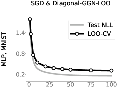
The first panel in Fig. 5 shows a good match between the above LOO estimate and test NLL. For comparison, in the next two panels, we show results for SGD training by using two ad-hoc measures obtained by plugging different Hessian approximations in Eq. 11. The first panel approximates $\mbox{$\mbox{$\mathbf{H}$}$}_{t}$ with a diagonal Generalized Gauss-Newton (GGN) matrix, while the second panel uses a K-FAC approximation. We see that diagonal-GGN-LOO does not work well at all and, while K-FAC-LOO improves this, it is still not as good as the iBLR result despite using a non-diagonal Hessian approximation. Not to mention, the two measures require an additional pass through the data to compute the Hessian approximation, and also need a careful setting of a damping parameter.

A similar result for iBLR is shown in Fig. 1(b) where we use the larger ResNet–20 on CIFAR10, and more such results are included in Fig. 8 of Sec. I.5. We also find that both diagonal-GGN-LOO or K-FAC-LOO further deteriorate when the model overfits; see Fig. 9. Results for the Adam optimizer are included in Fig. 10, where we again see that using ad hoc measures may not always work. Overall, these results show the difficulty of estimating sensitivity during training and suggest to take caution when using measures that are not naturally suited to analyze the training algorithm.

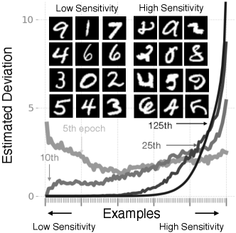
Evolution of sensitivities during training: Fig. 3(b) shows the evolution of sensitivities of examples as the training progresses. We use the iBLR algorithm and approximate the deviation as $\smash{\mbox{$\sigma$}(f_{i}(\mbox{$\mbox{$\mathbf{m}$}$}_{t}^{\backslash i}))-\mbox{$\sigma$}(f_{i}(\mbox{$\mbox{$\mathbf{m}$}$}_{t}))\approx\mbox{$\sigma$}^{\prime}(f_{i}(\mbox{$\mbox{$\mathbf{m}$}$}_{t}))v_{it}e_{it}}$ where $v_{it}$ and $e_{it}$ are obtained similarly to Eq. 16. The x-axis corresponds to examples sorted from least sensitive to most sensitive examples at convergence. The y-axis shows the histogram of sensitivity estimates. We observe that, as the training progresses, the distribution concentrates around a small fraction of the data. At the top, we visualize a few examples with high and low sensitivity estimates, where the high-sensitivity examples included interesting cases (similarly to Fig. 2). The result suggests that the model concentrates more and more on a small fraction of high-sensitivity examples, and therefore such examples can be used to characterize the model’s memory. Additional experiments of this kind are included in Fig. 11 of Sec. I.6, along with other experiment details.

We present the memory-perturbation equation by building upon the BLR framework. The equation suggests to take a step in the direction of the natural gradient of the perturbed examples. Using the MPE framework, we unify existing influence measures, generalize them to a wide variety of problems, and unravel useful properties regarding sensitivity. We also show that sensitivity estimation can be done cheaply and use this to predict generalization performance. An interesting avenue for future research is to apply the method to larger models and real-world problems. We also need to understand how our generalization measure compares to other methods, such as those considered in [22]. We would also like to understand the effect of various posterior approximations. Another interesting direction is to apply the method to non-Gaussian cases, for example, to study ensemble methods in deep learning with mixture models.

Acknowledgements

This work is supported by the Bayes duality project, JST CREST Grant Number JPMJCR2112.

References

- [1] Vincent Adam, Paul Chang, Mohammad Emtiyaz Khan, and Arno Solin. Dual Parameterization of Sparse Variational Gaussian Processes. Advances in Neural Information Processing Systems, 2021.
- [2] Chirag Agarwal, Daniel D’Souza, and Sara Hooker. Estimating Example Difficulty using Variance of Gradients. In Proceedings of the IEEE Conference on Computer Vision and Pattern Recognition, 2022.
- [3] Devansh Arpit, Stanisław Jastrzębski, Nicolas Ballas, David Krueger, Emmanuel Bengio, Maxinder S Kanwal, Tegan Maharaj, Asja Fischer, Aaron Courville, Yoshua Bengio, and Simon Lacoste-Julien. A Closer Look at Memorization in Deep Networks. In International Conference on Machine Learning, 2017.
- [4] Gregor Bachmann, Thomas Hofmann, and Aurélien Lucchi. Generalization Through The Lens of Leave-One-Out Error. In International Conference on Learning Representations, 2022.
- [5] Samyadeep Basu, Phil Pope, and Soheil Feizi. Influence Functions in Deep Learning Are Fragile. In International Conference on Learning Representations, 2021.
- [6] Christopher M. Bishop. Pattern Recognition and Machine Learning. Springer, 2006.
- [7] R Dennis Cook. Detection of Influential Observation in Linear Regression. Technometrics, 1977.
- [8] R Dennis Cook and Sanford Weisberg. Characterizations of an Empirical Influence Function for Detecting Influential Cases in Regression. Technometrics, 1980.
- [9] R Dennis Cook and Sanford Weisberg. Residuals and Influence in Regression. Chapman and Hall, 1982.
- [10] Corinna Cortes and Vladimir Vapnik. Support-Vector Networks. Machine learning, 1995.
- [11] Erik Daxberger, Agustinus Kristiadi, Alexander Immer, Runa Eschenhagen, Matthias Bauer, and Philipp Hennig. Laplace Redux-Effortless Bayesian Deep Learning. Advances in Neural Information Processing Systems, 2021.
- [12] Gintare Karolina Dziugaite and Daniel M Roy. Computing Nonvacuous Generalization Bounds for Deep (Stochastic) Neural Networks with Many More Parameters Than Training Data. In Proceedings of the Conference on Uncertainty in Artificial Intelligence, 2017.
- [13] Vitaly Feldman and Chiyuan Zhang. What Neural Networks Memorize and Why: Discovering the Long Tail via Influence Estimation. In Advances in Neural Information Processing Systems, 2020.
- [14] Wing K Fung and CW Kwan. A Note on Local Influence Based on Normal Curvature. Journal of the Royal Statistical Society: Series B (Statistical Methodology), 1997.
- [15] Ryan Giordano, Tamara Broderick, and Michael I Jordan. Covariances, robustness and variational Bayes. Journal of Machine Learning Research, 19(51), 2018.
- [16] Satoshi Hara, Atsushi Nitanda, and Takanori Maehara. Data Cleansing for Models Trained with SGD. In Advances in Neural Information Processing Systems, 2019.
- [17] Hrayr Harutyunyan, Alessandro Achille, Giovanni Paolini, Orchid Majumder, Avinash Ravichandran, Rahul Bhotika, and Stefano Soatto. Estimating Informativeness of Samples with Smooth Unique Information. In International Conference on Learning Representations, 2021.
- [18] James Hensman, Nicolo Fusi, and Neil D Lawrence. Gaussian Processes for Big Data. In Proceedings of the Conference on Uncertainty in Artificial Intelligence, 2013.
- [19] Alexander Immer, Matthias Bauer, Vincent Fortuin, Gunnar Rätsch, and Mohammad Emtiyaz Khan. Scalable Marginal Likelihood Estimation for Model Selection in Deep Learning. In International Conference on Machine Learning, 2021.
- [20] Alexander Immer, Maciej Korzepa, and Matthias Bauer. Improving Predictions of Bayesian Neural Nets via Local Linearization. International Conference on Artificial Intelligence and Statistics, 2021.
- [21] Louis A Jaeckel. The Infinitesimal Jackknife. Technical report, Bell Lab., 1972.
- [22] Yiding Jiang, Behnam Neyshabur, Hossein Mobahi, Dilip Krishnan, and Samy Bengio. Fantastic Generalization Measures and Where To Find Them. In International Conference on Learning Representations, 2020.
- [23] Angelos Katharopoulos and Francois Fleuret. Not All Samples Are Created Equal: Deep Learning with Importance Sampling. In International Conference on Machine Learning, 2018.
- [24] Mohammad Emtiyaz Khan. Variational Bayes Made Easy. Fifth Symposium on Advances in Approximate Bayesian Inference, 2023.
- [25] Mohammad Emtiyaz Khan, Alexander Immer, Ehsan Abedi, and Maciej Korzepa. Approximate Inference Turns Deep Networks into Gaussian Processes. Advances in Neural Information Processing Systems, 2019.
- [26] Mohammad Emtiyaz Khan and Wu Lin. Conjugate-Computation Variational Inference: Converting Variational Inference in Non-Conjugate Models to Inferences in Conjugate Models. In International Conference on Artificial Intelligence and Statistics, 2017.
- [27] Mohammad Emtiyaz Khan, Didrik Nielsen, Voot Tangkaratt, Wu Lin, Yarin Gal, and Akash Srivastava. Fast and Scalable Bayesian Deep Learning by Weight-Perturbation in Adam. In International Conference on Machine Learning, 2018.
- [28] Mohammad Emtiyaz Khan and Håvard Rue. The Bayesian Learning Rule. Journal of Machine Learning Research, 2023.
- [29] George S Kimeldorf and Grace Wahba. A Correspondence Between Bayesian Estimation on Stochastic Processes and Smoothing by Splines. The Annals of Mathematical Statistics, 1970.
- [30] Diederik Kingma and Jimmy Ba. Adam: A Method for Stochastic Optimization. In International Conference on Learning Representations, 2015.
- [31] Pang Wei Koh, Kai-Siang Ang, Hubert Teo, and Percy S Liang. On the Accuracy of Influence Functions for Measuring Group Effects. In Advances in Neural Information Processing Systems, 2019.
- [32] Pang Wei Koh and Percy Liang. Understanding Black-Box Predictions via Influence Functions. In International Conference on Machine Learning, 2017.
- [33] Aran Komatsuzaki. One Epoch is All You Need. ArXiv e-Prints, 2019.
- [34] Pierre-Simon Laplace. Mémoires de Mathématique et de Physique. Tome Sixieme, 1774.
- [35] Wu Lin, Mark Schmidt, and Mohammad Emtiyaz Khan. Handling the Positive-Definite Constraint in the Bayesian Learning Rule. In International Conference on Machine Learning, 2020.
- [36] Ilya Loshchilov and Frank Hutter. Decoupled Weight Decay Regularization. International Conference on Learning Representations, 2019.
- [37] David JC MacKay. Information Theory, Inference and Learning Algorithms. Cambridge University Press, 2003.
- [38] Roman Novak, Yasaman Bahri, Daniel A Abolafia, Jeffrey Pennington, and Jascha Sohl-Dickstein. Sensitivity and Generalization in Neural Networks: An Empirical Study. In International Conference on Learning Representations, 2018.
- [39] Kazuki Osawa, Satoki Ishikawa, Rio Yokota, Shigang Li, and Torsten Hoefler. ASDL: A Unified Interface for Gradient Preconditioning in PyTorch. In NeurIPS Workshop Order up! The Benefits of Higher-Order Optimization in Machine Learning, 2023.
- [40] Mansheej Paul, Surya Ganguli, and Gintare Karolina Dziugaite. Deep Learning on a Data Diet: Finding Important Examples Early in Training. In Advances in Neural Information Processing Systems, 2021.
- [41] Daryl Pregibon. Logistic Regression Diagnostics. The Annals of Statistics, 1981.
- [42] Garima Pruthi, Frederick Liu, Satyen Kale, and Mukund Sundararajan. Estimating Training Data Influence by Tracing Gradient Descent. In Advances in Neural Information Processing Systems, 2020.
- [43] Kamiar Rahnama Rad and Arian Maleki. A Scalable Estimate of the Out-of-Sample Prediction Error via Approximate Leave-One-Out Cross-Validation. Journal of the Royal Statistical Society Series B: Statistical Methodology, 2020.
- [44] Danilo Jimenez Rezende, Shakir Mohamed, and Daan Wierstra. Stochastic Backpropagation and Approximate Inference in Deep Generative Models. In International Conference on Machine Learning, 2014.
- [45] Hugh Salimbeni, Stefanos Eleftheriadis, and James Hensman. Natural Gradients in Practice: Non-Conjugate Variational Inference in Gaussian Process Models. In International Conference on Artificial Intelligence and Statistics, 2018.
- [46] Frank Schneider, Lukas Balles, and Philipp Hennig. DeepOBS: A Deep Learning Optimizer Benchmark Suite. In International Conference on Learning Representations, 2019.
- [47] Bernhard Schölkopf, Ralf Herbrich, and Alex J Smola. A Generalized Representer Theorem. In International Conference on Computational Learning Theory, 2001.
- [48] Saurabh Singh and Shankar Krishnan. Filter Response Normalization Layer: Eliminating Batch Dependence in the Training of Deep Neural Networks. In Proceedings of the IEEE Conference on Computer Vision and Pattern Recognition, 2020.
- [49] Ryutaro Tanno, Melanie F Pradier, Aditya Nori, and Yingzhen Li. Repairing Neural Networks by Leaving the Right Past Behind. Advances in Neural Information Processing Systems, 2022.
- [50] Luke Tierney and Joseph B Kadane. Accurate Approximations for Posterior Moments and Marginal Densities. Journal of the American Statistical Association, 1986.
- [51] Mariya Toneva, Alessandro Sordoni, Remi Tachet des Combes, Adam Trischler, Yoshua Bengio, and Geoffrey J. Gordon. An Empirical Study of Example Forgetting during Deep Neural Network Learning. In International Conference on Learning Representations, 2019.
- [52] Robert Weiss. An Approach to Bayesian Sensitivity Analysis. Journal of the Royal Statistical Society Series B: Statistical Methodology, 1996.
- [53] Fuzhao Xue, Yao Fu, Wangchunshu Zhou, Zangwei Zheng, and Yang You. To Repeat or Not To Repeat: Insights from Scaling LLM under Token-Crisis. ArXiv e-Prints, 2023.
- [54] Hongtu Zhu, Joseph G. Ibrahim, Sikyum Lee, and Heping Zhang. Perturbation Selection and Influence Measures in Local Influence Analysis. The Annals of Statistics, 2007.
Appendix A Influence Function for Linear Regression
We consider input-output pairs . The feature matrix containing as rows is denoted by and the output vector of length is denoted by . The loss is for . The regularizer is assumed to be . The minimizer is given by