The Manifold Of Variations:
hazard assessment of short-term impactors

Alessio Del Vigna Space Dynamics Services s.r.l., Via Mario Giuntini, Navacchio di Cascina, Pisa, Italy [email protected] Dipartimento di Matematica, Università di Pisa, Largo Bruno Pontecorvo 5, 56127 Pisa, Italy

Abstract.

When an asteroid has a few observations over a short time span the information contained in the observational arc could be so little that a full orbit determination may be not possible. One of the methods developed in recent years to overcome this problem is based on the systematic ranging and combined with the Admissible Region theory to constrain the poorly-determined topocentric range and range-rate. The result is a set of orbits compatible with the observations, the Manifold Of Variations, a 2-dimensional compact manifold parametrized over the Admissible Region. Such a set of orbits represents the asteroid confidence region and is used for short-term hazard predictions. In this paper we review the Manifold Of Variations method and make a detailed analysis of the related probabilistic formalism.

1. Introduction

An asteroid just discovered has a strongly undetermined orbit, being it weakly constrained by the few available astrometric observations. This is called a Very Short Arc (VSA, Milani et al. (2004)) since the observations cover a short time span. As it is well-known, the few observations constrain the position and velocity of the object in the sky-plane, but leave almost unknown the distance from the observer and the radial velocity, respectively the topocentric range and range-rate. This means that the asteroid confidence region is wide in at least two directions instead of being elongated and thin. Thus one-dimensional sampling methods, such as the use of the Line Of Variations (LOV, Milani et al. (2005)), are not a reliable representation of the confidence region. Indeed, VSAs are often too short to allow a full orbit determination, which would make it impossible even to define the LOV. To overcome the problem three systems have been developed in recent years: Scout at the NASA JPL (Farnocchia et al., 2015), NEOScan at SpaceDyS and at the University of Pisa (Spoto et al., 2018; Del Vigna, 2018), and neoranger at the University of Helsinki (Solin and Granvik, 2018).

Scout¹¹1https://cneos.jpl.nasa.gov/scout/ and NEOScan²²2https://newton.spacedys.com/neodys2/NEOScan/ are based on the systematic ranging, an orbit determination method which explores a suitable subset of the topocentric range and range-rate space (Chesley, 2005). They constantly scan the Minor Planet Center NEO Confirmation Page (NEOCP), with the goal of identifying asteroids such as NEAs, MBAs or distant objects to confirm/remove from the NEOCP and to give early warning of imminent impactors. NEOScan uses a method based on the systematic ranging and on the Admissible Region (AR) theory (Milani et al., 2004) to include in the orbit determination process also the information contained in the short arc, although too little to constrain a full orbit. Starting from a sampling of the AR, a set of orbits compatible with the observations is then computed by a doubly constrained differential correction technique, which in turn ends with a sampling of the Manifold Of Variations (MOV, Tommei (2006)), a 2-dimensional manifold of orbits parametrized over the AR and representing a two-dimensional analogue of the LOV. This combination of techniques provided a robust short-term orbit determination method and also a two-dimensional sampling of the confidence region to use for the subsequent hazard assessment and for the planning of the follow-up activity of interesting objects.

In this paper we review the algorithm at the basis of NEOScan and examine in depth the underlying mathematical formalism, focusing on the short-term impact monitoring and the impact probability computation. In Section 2 we summarise the AR theory and the main definitions concerning the MOV. Section 3 contains the results for the derivation of the probability density function on an appropriate integration space, by assuming that the residuals are normally distributed and by a suitable linearisation. In Section 4 we show that without the linearisation assumed in the previous section we find a distribution known to be inappropriate for the problem of computing the impact probability of short-term impactors (Farnocchia et al., 2015). In Section 5 we give a probabilistic interpretation to the optimisation method used to define the MOV, namely the doubly constrained differential corrections. Lastly, Section 6 contains our conclusions and a possible application of the method presented in this paper to study in future research.

2. The Admissible Region and the Manifold Of Variations

As anticipated in the introduction, the systematic ranging method on which NEOScan is based makes a deep use of the Admissible Region. In this section we briefly recap its main properties and we refer the reader to relevant further references.

When in presence of a VSA, even when we are not able to fit a full least squares orbit, we are anyway able to compute the right ascension $\alpha$ , the declination $\delta$ , and their time derivatives $\dot{\alpha}$ and $\dot{\delta}$ , to form the so-called attributable (Milani et al., 2004). For the notation, we indicate the attributable as

\mathcal{A}\coloneqq(\alpha,\delta,\dot{\alpha},\dot{\delta})\in\mathbb{S}^{1}\times\left(-\tfrac{\pi}{2},\tfrac{\pi}{2}\right)\times\mathbb{R}^{2},

where all the quantities are referred to the mean of the observational times. The AR has been introduced to constrain the possible values of the range $\rho$ and the range-rate $\dot{\rho}$ that the attributable leaves completely undetermined. Among other things, we require that the observed object is a Solar System body, discarding the orbits corresponding to too small objects to be source of meteorites (the so-called shooting star limit).

The AR turns out to be a compact subset of $\mathbb{R}_{\geq 0}\times\mathbb{R}$ and to have at most two connected components. Commonly the AR has one component and the case with two components indicates the possibility for the asteroid to be distant. Since the AR is compact we can sample it with a finite number of points, and we use two different sampling techniques depending on the geometric properties of the AR and on the existence of a reliable least squares orbit. A nominal solution is an orbit obtained by unconstrained (i.e. full) differential corrections, starting from a preliminary orbit as first guess. Indeed it does happen that the available observations are enough to constrain a full orbit: it essentially depends on the quality of the observed arc, which can be measured by the arc type and the signal-to-noise ratio of the geodesic curvature of the arc on the celestial sphere (Milani et al., 2007). We say that the nominal orbit is reliable if the latter is $>3$ . If this is the case we anyway compute a sampling of orbits compatible with the observations to use to make predictions, but instead of considering the entire AR we exploit the knowledge of the least squares orbit, and in particular of its covariance.
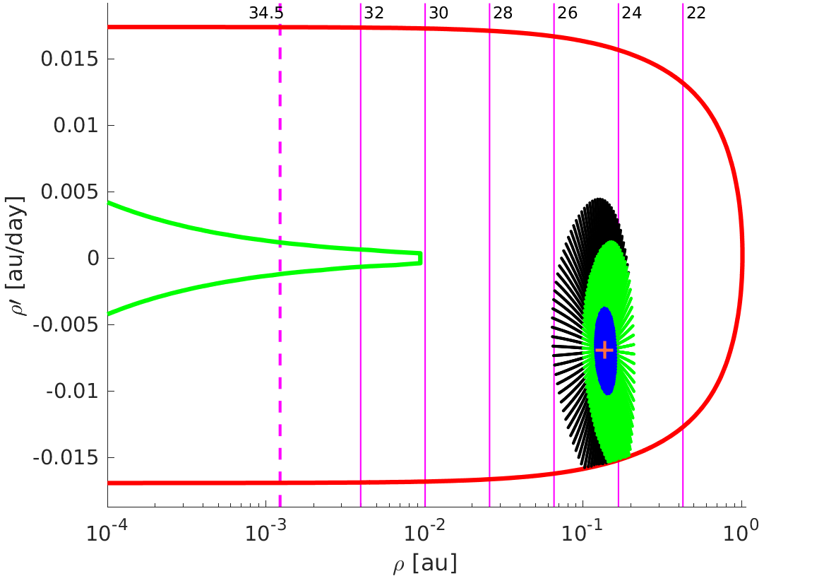
Grid sampling. When a reliable nominal solution does not exist or it is not reliable, the systematic ranging is performed by a two-step procedure and in both steps it uses rectangular grids over the AR. In the first step a grid covers the entire AR, with the sample points for $\rho$ spaced either uniformly or with a logarithmic scale depending on the geometry of the AR (see Figure 1, left). The corresponding sampling of the MOV is then computed, with the doubly constrained differential corrections procedure described below. Then we are able to identify the orbits which are more compatible with the observations by computing their $\chi^{2}$ value (see Equation (2.2)), and we can restrict the grid to the region occupied by such orbits. Thus the grid used in the second step typically covers a smaller region and thus it has a higher resolution than the first one (see Figure 1, right).
Cobweb sampling. If a reliable nominal orbit exists, instead of using a grid we compute a spider web sampling in a suitable neighbourhood of the nominal solution. This is obtained by following the level curves of the quadratic approximation of the target function used to minimise the RMS of the observational residuals (see Figure 2).
For the formal definition of the AR and the proof of its properties the reader can refer to Milani et al. (2004). The operative definition used in NEOScan and a detailed explanation of the sampling techniques can be found in Spoto et al. (2018) and Del Vigna (2018).

Refer to caption — Figure 1. Admissible Region sampling with the rectangular grids. *Left*. AR sampling performed with the first grid, covering the whole AR. *Right*. Sampling of the region containing the orbits with $\chi<5$ resulting from the first grid. In both plots the sample points are marked in blue when $\chi\leq 2$ and in green when $2<\chi<5$ .

We now describe the Manifold Of Variations, a sample of orbits compatible with the observational data set. In general, to obtain orbits from observations we use the least squares method. The target function is

Q(\mathbf{x})\coloneqq\frac{1}{m}\bm{\xi}(\mathbf{x})^{\top}W\bm{\xi}(\mathbf{x}),

where $\mathbf{x}$ are the orbital elements to fit, $m$ is the number of observations used, $\bm{\xi}$ is the vector of the observed-computed debiased astrometric residuals, and $W$ is the weight matrix. As explained in the introduction, in general a full orbit determination is not possible for short arcs. Nevertheless, from the observational data set it is possible to compute an attributable $\mathcal{A}_{0}$ . The AR theory has been developed to obtain constraints on the values of $(\rho,\dot{\rho})$ , so that we can merge the information contained in the attributable with the knowledge of an AR sampling. The basic idea of this method is to fix $\rho$ and $\dot{\rho}$ at some specific values $\bm{\rho}_{0}=(\rho_{0},\dot{\rho}_{0})$ obtained from the AR sampling, compose the full orbit $(\mathcal{A}_{0},\bm{\rho}_{0})$ , and fit only the attributable part to the observations with a suitable differential corrections procedure.

Definition 2.1.

Given a subset $K$ of the AR, we define the Manifold Of Variations to be the set of points $(\mathcal{A}^{*}(\bm{\rho}_{0}),\bm{\rho}_{0})$ such that $\bm{\rho}_{0}\in K$ and $\mathcal{A}^{*}(\bm{\rho}_{0})$ is the local minimum of the function $\left.Q(\mathcal{A},\bm{\rho})\right|_{\bm{\rho}=\bm{\rho}_{0}}$ , when it exists. We denote the Manifold Of Variations with $\mathcal{M}$ .

Remark 2.2.

In general $\mathcal{M}$ is a 2-dimensional manifold, since the differential of the map from the $(\rho,\dot{\rho})$ space to $\mathcal{M}$ has rank $2$ (see Lemma 3.2).

The set $K$ is the intersection of a rectangle with the AR in the case of the grid sampling, whereas $K$ is an ellipse around $\bm{\rho}^{*}$ in the cobweb case, where $\mathbf{x}^{*}=(\mathcal{A}^{*},\bm{\rho}^{*})$ is the reliable nominal orbit. To fit the attributable part we use the doubly constrained differential corrections, which are usual differential corrections but performed on a 4-dimensional space rather than on a 6-dimensional one. The normal equation is

C_{\mathcal{A}}\Delta\mathcal{A}=D_{\mathcal{A}},

where

C_{\mathcal{A}}\coloneqq B_{\mathcal{A}}^{\top}WB_{\mathcal{A}}\,,\quad D_{\mathcal{A}}\coloneqq-B_{\mathcal{A}}^{\top}W\bm{\xi}\,,\quad B_{\mathcal{A}}\coloneqq\frac{\partial{\bm{\xi}}}{\partial{\mathcal{A}}}.

(2.1)

We call $K^{\prime}$ the subset of $K$ on which the doubly constrained differential corrections converge, giving a point on $\mathcal{M}$ .

Definition 2.3.

For each orbit $\mathbf{x}\in\mathcal{M}$ we define the $\chi$ -value to be

{}\chi(\mathbf{x})\coloneqq\sqrt{m(Q(\mathbf{x})-Q^{*})},

(2.2)

where $Q^{*}$ is the minimum value of the target function over $K^{\prime}$ , that is $Q^{*}\coloneqq\min_{\bm{\rho}\in K^{\prime}}Q(\mathcal{A}^{*}(\bm{\rho}),\bm{\rho})$ . The orbit for which this minimum is attained is denoted with $\mathbf{x}^{*}$ and referred to as the best-fitting orbit.

The standard differential corrections are a variant of the Newton method to find the minimum of a multivariate function, the target function $Q$ (Milani and Gronchi, 2010). The uncertainty of the result can be described in terms of confidence ellipsoids (optimisation interpretation) as well as in the language of probability (probabilistic interpretation). In Section 5 we give a probabilistic interpretation to the doubly constrained differential corrections procedure.

3. Derivation of the probability density function

Starting from Spoto et al. (2018) we now give the proper mathematical formalism to derive the probability density function on a suitable space $S$ which we define below. Upon integration this will lead to accurate probability estimates, the most important and urgent of which is the impact probability computation for a possible imminent impactor.

Our starting point is a probability density function on the residuals space, to propagate back to $S$ . In particular, we assume the residuals to be distributed according to a Gaussian random variable $\bm{\Xi}$ , with zero mean and covariance $\Gamma_{\bm{\xi}}=W^{-1}$ , that is

p_{\bm{\Xi}}(\bm{\xi})=N(\bm{0},\Gamma_{\bm{\xi}})(\bm{\xi})=\frac{\sqrt{\det W}}{(2\pi)^{m/2}}\exp\left(-\frac{mQ(\bm{\xi})}{2}\right)=\frac{\sqrt{\det W}}{(2\pi)^{m/2}}\exp\left(-\frac{1}{2}\bm{\xi}^{\top}W\bm{\xi}\right).

Without loss of generality, we can assume that

p_{\bm{\Xi}}(\bm{\xi})=N(\bm{0},I_{m})(\bm{\xi})=\frac{1}{(2\pi)^{m/2}}\exp\left(-\frac{1}{2}\bm{\xi}^{\top}\bm{\xi}\right),

(3.1)

where $I_{m}$ is the $m\times m$ identity matrix. This is obtained by using the normalised residuals in place of the true residuals (see for instance Milani and Gronchi (2010)). For the notation, from now on we will use $\bm{\xi}$ to indicate the normalised residuals. Note that with the use of normalised residuals the target function becomes $Q(\mathbf{x})=\frac{1}{m}\bm{\xi}(\mathbf{x})^{\top}\bm{\xi}(\mathbf{x})$ .

3.1. Spaces and maps

Let us introduce the following spaces.

(i)

$S$ is the sampling space, which is $\mathbb{R}_{\geq 0}\times\mathbb{R}$ if the sampling is uniform in $\rho$ , $\mathbb{R}^{2}$ if the sampling is uniform in $\log_{10}\rho$ , and $\mathbb{R}_{\geq 0}\times\mathbb{S}^{1}$ in the cobweb case.
(ii)

$K^{\prime}\subseteq\mathbb{R}_{\geq 0}\times\mathbb{R}$ has already been introduced in Section 2, and it is the subset of the points of the AR on which the doubly constrained differential corrections achieved convergence.
(iii)

$\mathcal{X}\coloneqq A\times R$ is the orbital elements space in attributable coordinates, where $A\coloneqq\mathbb{S}^{1}\times(-\pi/2,\pi/2)\times\mathbb{R}^{2}$ is the attributable space and $R\coloneqq\mathbb{R}_{\geq 0}\times\mathbb{R}$ is the range/range-rate space.
(iv)

$\mathcal{M}$ is the Manifold Of Variations, a 2-dimensional submanifold of $\mathcal{X}$ .
(v)

$\mathbb{R}^{m}$ is the residuals space, whose dimension is $m\geq 6$ since the number of observations must be $\geq 3$ .

We now define the maps we use to propagate back the density $p_{\bm{\Xi}}$ . First, the residuals are a function of the fit parameters, that is $\bm{\xi}=F(\mathbb{x})$ , with $F:\mathcal{X}\rightarrow\mathbb{R}^{m}$ being a differentiable map. The second map goes from the AR space to the MOV space.

Definition 3.1.

The map $f_{\mu}:K^{\prime}\rightarrow\mathcal{M}$ is defined to be

f_{\mu}(\bm{\rho})\coloneqq(\mathcal{A}^{*}(\bm{\rho}),\bm{\rho}),

where $\mathcal{A}^{*}(\bm{\rho})\in A$ is the best-fit attributable obtained at convergence of the doubly constrained differential corrections.

Lemma 3.2.

The map $f_{\mu}$ is a global parametrization of $\mathcal{M}$ as a $2$ -dimensional manifold.

Proof.

The set $K^{\prime}$ is a subset of $\mathbb{R}^{2}$ with non-empty interior, the map $f_{\mu}$ is at least $C^{1}$ and its Jacobian matrix is

(Df_{\mu})_{\bm{\rho}}=\frac{\partial f_{\mu}}{\partial\bm{\rho}}(\bm{\rho})=\begin{pmatrix}\dfrac{\partial\mathcal{A}^{*}}{\partial\bm{\rho}}(\bm{\rho})\\[8.5359pt] I_{2}\end{pmatrix},

(3.2)

from which is clear that it is full rank on $K^{\prime}$ . ∎

The last map to introduce is that from the sampling space $S$ to the AR space $R$ .

Definition 3.3.

The map $f_{\sigma}:S\rightarrow R$ is defined according to the sampling technique:

(i)

if the sampling is uniform in $\rho$ , $f_{\sigma}$ is the identity map;
(ii)

if the sampling is uniform in $\log_{10}\rho$ , we have $S=\mathbb{R}^{2}$ and $f_{\sigma}(x,y)\coloneqq(10^{x},y)$ ;

(iii)

if we are in the cobweb case, $S=\mathbb{R}_{\geq 0}\times\mathbb{S}^{1}$ and the map $f_{\sigma}$ is given by

f_{\sigma}(r,\theta)\coloneqq r\begin{pmatrix}\sqrt{\lambda_{1}}\cos{\theta}&-\sqrt{\lambda_{2}}\sin{\theta}\\ \sqrt{\lambda_{2}}\sin{\theta}&\phantom{-}\sqrt{\lambda_{1}}\cos{\theta}\end{pmatrix}\mathbf{v}_{1}+\begin{pmatrix}\rho^{*}\\ \dot{\rho}^{*}\end{pmatrix},\

where $\lambda_{1}>\lambda_{2}$ are the eigenvalues of the $2\times 2$ matrix $\Gamma_{\bm{\rho}\bm{\rho}}(\mathbf{x}^{*})$ , the latter being the restriction of the covariance matrix $\Gamma(\mathbf{x}^{*})$ to the $(\rho,\dot{\rho})$ space, and $\mathbf{v_{1}}$ is the unit eigenvector corresponding to $\lambda_{1}$ .

We then consider the following chain of maps

S\overset{f_{\sigma}}{\longrightarrow}R\supseteq K^{\prime}\overset{f_{\mu}}{\longrightarrow}\mathcal{M}\subseteq\mathcal{X}\overset{F}{\longrightarrow}\mathbb{R}^{m}

and we use it to compute the probability density function on $S$ obtained by propagating $p_{\bm{\Xi}}$ back.

3.2. Conditional density of a Gaussian on an affine subspace

In this section we establish general results about the conditional probability density function of a Gaussian random variable on an affine subspace. Let $m$ and $N$ be two positive integers, with $m>N$ . Let $B\in{\bf M}_{m,N}(\mathbb{R})$ a $m\times N$ matrix with full rank, that is $\operatorname{rk}(B)=N$ . Consider the affine $N$ -dimensional subspace of $\mathbb{R}^{m}$ given by

W\coloneqq\left\{\bm{\xi}\in\mathbb{R}^{m}\,:\,\bm{\xi}=B\mathbf{x}+\bm{\xi}^{*},\ \mathbf{x}\in\mathbb{R}^{N}\right\}=\operatorname{Imm}(B)+\bm{\xi}^{*}.

We can also assume that $\bm{\xi}^{*}$ is orthogonal to $W$ , that is $\bm{\xi}^{*}\in\operatorname{Imm}(B)^{\perp}$ , otherwise it is possible to subtract the component parallel to $W$ . Given the random variable $\bm{\Xi}$ with the Gaussian distribution on $\mathbb{R}^{m}$ as in (3.1), we want to find the conditional probability density $p_{\bm{\Xi}|W}$ of $\bm{\Xi}$ on $W$ . Let $R\in{\bf M}_{m}(\mathbb{R})$ be a $m\times m$ rotation matrix and let $f_{R}:\mathbb{R}^{m}\rightarrow\mathbb{R}^{m}$ be the affine map

f_{R}(\bm{\xi})\coloneqq R(\bm{\xi}-\bm{\xi}^{*}).

Throughout this section, we use the notation $f_{R}(\bm{\xi})\eqqcolon\bm{\xi}_{R}=\begin{pmatrix}\bm{\xi}^{\prime}\\ \bm{\xi}^{\prime\prime}\end{pmatrix}$ , with $\bm{\xi}^{\prime}\in\mathbb{R}^{m-N}$ and $\bm{\xi}^{\prime\prime}\in\mathbb{R}^{N}$ . We choose $R$ in such a way that

f_{R}^{-1}\begin{pmatrix}\mathbf{0}\\ \bm{\xi}^{\prime\prime}\end{pmatrix}=R^{\top}\begin{pmatrix}\mathbf{0}\\ \bm{\xi}^{\prime\prime}\end{pmatrix}+\bm{\xi}^{*}\in W\quad\text{for all $\bm{\xi}^{\prime\prime}\in\mathbb{R}^{N}$}.

(3.3)

Lemma 3.4.

Condition (3.3) holds for all $\bm{\xi}^{\prime\prime}\in\mathbb{R}^{N}$ if and only if there exists an invertible matrix $A\in{\bf M}_{N}(\mathbb{R})$ such that $RB=\begin{pmatrix}0\\ A\end{pmatrix}$ .

Proof.

$(\Leftarrow)$ Let $\begin{pmatrix}\mathbf{0}\\ \bm{\xi}^{\prime\prime}\end{pmatrix}\in\mathbb{R}^{m}$ . Since $A$ is invertible there exists $\tilde{\mathbf{x}}\in\mathbb{R}^{N}$ such that $A\tilde{\mathbf{x}}=\bm{\xi}^{\prime\prime}$ . Then $R^{\top}\begin{pmatrix}\mathbf{0}\\ \bm{\xi}^{\prime\prime}\end{pmatrix}=R^{\top}\begin{pmatrix}0\\ A\end{pmatrix}\tilde{\mathbf{x}}=R^{\top}RB\tilde{\mathbf{x}}=B\tilde{\mathbf{x}}$ , hence $R^{\top}\begin{pmatrix}\mathbf{0}\\ \bm{\xi}^{\prime\prime}\end{pmatrix}+\bm{\xi}^{*}=B\tilde{\mathbf{x}}+\bm{\xi}^{*}\in W$ .
$(\Rightarrow)$ Condition (3.3) implies that for all $\bm{\xi}^{\prime\prime}\in\mathbb{R}^{N}$ there exists $\tilde{\mathbf{x}}\in\mathbb{R}^{N}$ such that $\begin{pmatrix}\mathbf{0}\\ \bm{\xi}^{\prime\prime}\end{pmatrix}=RB\tilde{\mathbf{x}}$ . Since the multiplication by $RB$ is injective, such $\tilde{\mathbf{x}}$ is unique. Therefore there exists a well-defined map $P:\mathbb{R}^{N}\rightarrow\mathbb{R}^{N}$ such that $P(\bm{\xi}^{\prime\prime})=\tilde{\mathbf{x}}$ . The map $P$ is linear and injective since $\operatorname{Ker}{P}=\{\mathbf{0}\}$ , thus it is a bijection. If $A$ is the $N\times N$ matrix associated to $P^{-1}$ , there easily follows $RB=\begin{pmatrix}0\\ A\end{pmatrix}$ . ∎

Lemma 3.5.

Let $U\coloneqq\{\bm{\xi}_{R}\in\mathbb{R}^{m}\,:\,\bm{\xi}^{\prime}=\mathbf{0}\}$ . Then the following holds:

(i)

$U=f_{R}(W)=R\operatorname{Imm}{B}$ and the map $\left.f_{R}\right|_{W}:W\rightarrow U$ is a bijection;
(ii)

$R\bm{\xi}^{*}=\begin{pmatrix}\bm{\xi}^{\prime*}\\ \mathbf{0}\end{pmatrix}$ for some $\bm{\xi}^{\prime*}\in\mathbb{R}^{m-N}$ .

Proof.

(i) The inclusion $U\subseteq f_{R}(W)$ is trivial. For the other one, let $\bm{\xi}\in W$ , then there exists $\tilde{\mathbf{x}}\in\mathbb{R}^{N}$ such that $\bm{\xi}=B\tilde{\mathbf{x}}+\bm{\xi}^{*}$ . From Lemma 3.4 we have $f_{R}(\bm{\xi})=RB\tilde{\mathbf{x}}=\begin{pmatrix}0\\ A\end{pmatrix}\tilde{\mathbf{x}}\in U$ .
(ii) Since $\bm{\xi}^{*}\in(\operatorname{Imm}{B})^{\perp}$ and $R$ is an isometry, we have $R\bm{\xi}^{*}\in R(\operatorname{Imm}{B})^{\perp}=(R\operatorname{Imm}{B})^{\perp}=U^{\perp}$ , where the last equality follows from (i). ∎∎

Theorem 3.6.

The conditional probability density of $\bm{\Xi}^{\prime\prime}$ is $N(\mathbf{0},I_{N})$ , that is

p_{\bm{\Xi}^{\prime\prime}}(\bm{\xi}^{\prime\prime})=\frac{1}{(2\pi)^{N/2}}\exp\left(-\frac{1}{2}\bm{\xi}^{\prime\prime\top}\bm{\xi}^{\prime\prime}\right)

Proof.

By the standard propagation formula for probability density functions under the action of a continuous function, we have that

	$\displaystyle p_{f_{R}(\bm{\Xi})}(\bm{\xi}_{R})$	$\displaystyle=\left\|\det R\right\|p_{\bm{\Xi}}(f_{R}^{-1}(\bm{\xi}_{R}))=$
		$\displaystyle=\frac{1}{(2\pi)^{m/2}}\exp\left(-\frac{1}{2}(R^{\top}\bm{\xi}_{R}+\bm{\xi}^{})^{\top}(R^{\top}\bm{\xi}_{R}+\bm{\xi}^{})\right)=$
		$\displaystyle=\frac{1}{(2\pi)^{m/2}}\exp\left(-\frac{1}{2}\left(\bm{\xi}_{R}^{\top}\bm{\xi}_{R}+2\bm{\xi}_{R}^{\top}R\bm{\xi}^{}+{\bm{\xi}^{}}^{\top}\bm{\xi}^{*}\right)\right).$

The conditional probability density of the variable $f_{R}(\bm{\Xi})$ on $f_{R}(W)=U$ (see Lemma 3.5-(i)) is obtained by using that $\bm{\xi}^{\prime}=\mathbf{0}$ and Lemma 3.5-(ii). We have

p_{f_{R}(\bm{\Xi})|f_{R}(W)}(\bm{\xi}^{\prime\prime})=\frac{\frac{1}{(2\pi)^{m/2}}\exp\left(-\frac{1}{2}\left(\bm{\xi}^{\prime\prime\top}\bm{\xi}^{\prime\prime}+{\bm{\xi}^{*}}^{\top}\bm{\xi}^{*}\right)\right)}{\int_{\mathbb{R}^{N}}\frac{1}{(2\pi)^{m/2}}\exp\left(-\frac{1}{2}\left(\bm{\xi}^{\prime\prime\top}\bm{\xi}^{\prime\prime}+{\bm{\xi}^{*}}^{\top}\bm{\xi}^{*}\right)\right)\,{\rm d}\bm{\xi}^{\prime\prime}}=\frac{1}{(2\pi)^{N/2}}\exp\left(-\frac{1}{2}\bm{\xi}^{\prime\prime\top}\bm{\xi}^{\prime\prime}\right),

where we have used that $\int_{\mathbb{R}^{n}}\exp\left(-\frac{1}{2}\mathbf{y}^{\top}\mathbf{y}\right)\,{\rm d}\mathbf{y}=(2\pi)^{n/2}$ for all $n\geq 1$ . Now the thesis follows by noting that the random variable $f_{R}(\bm{\Xi})|f_{R}(W)$ coincides with $\bm{\Xi}^{\prime\prime}$ . ∎∎

Corollary 3.7.

The conditional probability density of $\bm{\Xi}$ on $W$ is

p_{\bm{\Xi}|W}(\bm{\xi})=\frac{1}{(2\pi)^{N/2}}\exp\left(-\frac{1}{2}(\bm{\xi}-\bm{\xi}^{*})^{\top}(\bm{\xi}-\bm{\xi}^{*})\right),

where $\bm{\xi}\in W$ .

Proof.

From Lemma 3.5-(i) we know that $f_{R}|_{W}$ is a bijection. Thus for all $\bm{\xi}^{\prime\prime}\in\mathbb{R}^{N}$ there exists a unique $\bm{\xi}\in W$ such that $\begin{pmatrix}\mathbf{0}\\ \bm{\xi}^{\prime\prime}\end{pmatrix}=f_{R}(\bm{\xi})=R(\bm{\xi}-\bm{\xi}^{*})$ . Now it suffices to use this fact in the equation for $p_{\bm{\Xi}^{\prime\prime}}(\bm{\xi}^{\prime\prime})$ in Theorem 3.6. ∎∎

3.3. Computation of the probability density

We first derive the probability density function on the Manifold Of Variations from that on the normalised residuals space. The computation is based on the linearisation of the map $F$ around the best-fitting orbit. In Section 4 we will instead show the result of the full non-linear propagation of the probability density function and discuss the reason for which this approach, although correct, is not a suitable choice for applications.

Theorem 3.8.

Let $\mathbf{X}$ be the random variable of $\mathcal{X}$ . By linearising $F$ around the best-fitting orbit $\mathbf{x}^{*}$ , the conditional probability density of $\mathbf{X}$ on $T_{\mathbf{x}^{*}}\mathcal{M}$ is given by

p_{\mathbf{X}|T_{\mathbf{x}^{*}}\mathcal{M}}(\mathbf{x})=\dfrac{\displaystyle\exp\left(-\frac{\chi^{2}(\mathbf{x})}{2}\right)}{\displaystyle\int_{T_{\mathbf{x}^{*}}\mathcal{M}}\exp\left(-\frac{\chi^{2}(\mathbf{y})}{2}\right)\,{\rm d}\mathbf{y}}.

(3.4)

Proof.

The map $F$ is differentiable of class at least $C^{1}$ and the Jacobian matrix of $F$ is the design matrix $B(\mathbf{x})=\frac{\partial F}{\partial\mathbf{x}}(\mathbf{x})\in{\bf M}_{m,N}(\mathbb{R})$ . Since the doubly constrained differential corrections converge to $\mathbf{x}^{*}$ , the matrix $B(\mathbf{x}^{*})$ is full rank. It follows that the map $F$ is a local parametrization of

V\coloneqq F(\mathcal{M})=\{\bm{\xi}\in\mathbb{R}^{m}\,:\,\bm{\xi}=F(\mathbf{x}),\ \mathbf{x}\in\mathcal{M}\},

in a suitable neighbourhood of $\bm{\xi}^{*}\coloneqq F(\mathbf{x}^{*})=\xi(\mathbf{x}^{*})$ . The set $V$ is thus a 2-dimensional submanifold of the residuals space $\mathbb{R}^{m}$ . Consider the differential

DF_{\mathbf{x}^{*}}:T_{\mathbf{x}^{*}}\mathcal{M}\rightarrow T_{\bm{\xi}^{*}}V,

where $T_{\bm{\xi}^{*}}V=\{\bm{\xi}\in\mathbb{R}^{m}\,:\,\bm{\xi}=\bm{\xi}^{*}+B(\mathbf{x}^{*})(\mathbf{x}-\mathbf{x^{*}}),\,\mathbf{x}\in T_{\mathbf{x}^{*}}\mathcal{M}\}$ is a 2-dimensional affine subspace of $\mathbb{R}^{m}$ . We claim that $\bm{\xi}^{*}$ is orthogonal to $T_{\bm{\xi}^{*}}V$ : since $\mathbf{x}^{*}$ is a local minimum of the target function $Q$

\mathbf{0}=\frac{\partial Q}{\partial\mathbf{x}}(\mathbf{x}^{*})=\frac{2}{m}\bm{\xi}(\mathbf{x}^{*})^{\top}B(\mathbf{x}^{*}),

that is $\bm{\xi}(\mathbf{x}^{*})=\bm{\xi}^{*}\in\operatorname{Imm}\left(B(\mathbf{x}^{*})\right)^{\perp}$ . By applying Corollary 3.7 we have that

p_{\bm{\Xi}|T_{\bm{\xi}^{*}}V}(\bm{\xi})=\frac{1}{2\pi}\exp\left(-\frac{1}{2}(\bm{\xi}-\bm{\xi}^{*})^{\top}(\bm{\xi}-\bm{\xi}^{*})\right)

for $\bm{\xi}\in T_{\bm{\xi}^{*}}V$ . The differential map is continuous and invertible (since it is represented by the matrix $A(\mathbf{x}^{*})$ , as in Lemma 3.4), thus we can use the standard formula for the transformations of random variables to obtain

p_{\mathbf{X}|T_{\mathbf{x}^{*}}\mathcal{M}}(\mathbf{x})=\frac{\sqrt{\det C(\mathbf{x}^{*})}}{2\pi}\exp\left(-\frac{1}{2}(\mathbf{x}-\mathbf{x}^{*})^{\top}C(\mathbf{x}^{*})(\mathbf{x}-\mathbf{x}^{*})\right),

for $\mathbf{x}\in T_{\mathbf{x}^{*}}\mathcal{M}$ , where $C(\mathbf{x}^{*})$ is the $6\times 6$ normal matrix of the differential corrections converging to $\mathbf{x}^{*}$ . Furthermore, in the approximation used, we have

\chi^{2}(\mathbf{x})=mQ(\mathbf{x})-mQ^{*}=(\mathbf{x}-\mathbf{x}^{*})^{\top}C(\mathbf{x}^{*})(\mathbf{x}-\mathbf{x}^{*}),

so that for $\mathbf{x}\in T_{\mathbf{x}^{*}}\mathcal{M}$

p_{\mathbf{X}|T_{\mathbf{x}^{*}}\mathcal{M}}(\mathbf{x})=\frac{\sqrt{\det C(\mathbf{x}^{*})}}{2\pi}\exp\left(-\frac{\chi^{2}(\mathbf{x})}{2}\right).

Now the thesis follows by normalising the density just obtained. ∎∎

We now complete the derivation of the probability density function on the space $S$ . In particular, to obtain the density on the space $R$ we use the notion of integration over a manifold because we want to propagate a probability density on a manifold to a probability density over the space that parametrizes the manifold itself (see Theorem 3.9). Then the last step involves two spaces with the same dimension, namely $R$ and $S$ , thus we simply apply standard propagation results from probability density functions (see Theorem 3.10).

Theorem 3.9.

Let $\mathbf{R}$ be the random variable on the space $R$ . Assuming (3.4) to be the probability density function on $\mathcal{M}$ , the probability density function of $\mathbf{R}$ is

p_{\mathbf{R}}(\bm{\rho})=\dfrac{\displaystyle\exp\left(-\frac{\chi^{2}(\bm{\rho})}{2}\right)\sqrt{G_{\mu}(\bm{\rho})}}{\displaystyle\int_{K^{\prime}}\exp\left(-\frac{\chi^{2}(\bm{\rho})}{2}\right)\sqrt{G_{\mu}(\bm{\rho})}\,{\rm d}\bm{\rho}},

where $\chi^{2}(\bm{\rho})=\chi^{2}(\mathbf{x}(\bm{\rho}))$ and $G_{\mu}$ is the Gramian determinant

G_{\mu}(\bm{\rho})=\det\left(I_{2}+\left(\frac{\partial\mathcal{A}^{*}}{\partial\bm{\rho}}(\bm{\rho})\right)^{\top}\frac{\partial\mathcal{A}^{*}}{\partial\bm{\rho}}(\bm{\rho})\right).

Moreover, neglecting terms containing the second derivatives of the residuals multiplied by the residuals themselves, for all $\bm{\rho}\in K^{\prime}$ we have

\frac{\partial\mathcal{A}^{*}}{\partial\bm{\rho}}(\bm{\rho})=-C_{\mathcal{A}}(\mathcal{A}^{*}(\bm{\rho}),\bm{\rho})^{-1}B_{\mathcal{A}}(\mathcal{A}^{*}(\bm{\rho}),\bm{\rho})^{\top}B_{\bm{\rho}}(\mathcal{A}^{*}(\bm{\rho}),\bm{\rho}).

Proof.

We have already proved that the map $f_{\mu}:K^{\prime}\rightarrow\mathcal{M}$ is a global parametrization of $\mathcal{M}$ . From the definition of integral of a function over a manifold we have

p_{\mathbf{R}}(\bm{\rho})=p_{\mathbf{X}|T_{\mathbf{x}^{*}}\mathcal{M}}(f_{\mu}(\bm{\rho}))\cdot\sqrt{\det\left[\frac{\partial f_{\mu}}{\partial\bm{\rho}}(\bm{\rho})\right]^{\top}\frac{\partial f_{\mu}}{\partial\bm{\rho}}(\bm{\rho})}

and the thesis follows since from Equation (3.2)

\left[\frac{\partial f_{\mu}}{\partial\bm{\rho}}(\bm{\rho})\right]^{\top}\frac{\partial f_{\mu}}{\partial\bm{\rho}}(\bm{\rho})=I_{2}+\left(\dfrac{\partial\mathcal{A}^{*}}{\partial\bm{\rho}}(\bm{\rho})\right)^{\top}\dfrac{\partial\mathcal{A}^{*}}{\partial\bm{\rho}}(\bm{\rho}).

The equation for $\frac{\partial\mathcal{A}^{*}}{\partial\bm{\rho}}(\bm{\rho})$ is proved in Spoto et al. (2018), Appendix A, but for the sake of completeness we repeat the argument here. Let $\bm{\rho}\in K^{\prime}$ . By definition, the point $\mathbf{x}(\bm{\rho})=(\mathcal{A}^{*}(\bm{\rho}),\bm{\rho})\in\mathcal{M}$ is a zero of the function $g:\mathcal{X}\rightarrow\mathbb{R}$ defined to be

g(\mathbf{x})\coloneqq\frac{m}{2}\frac{\partial Q}{\partial\mathcal{A}}(\mathbf{x})=B_{\mathcal{A}}(\mathbf{x})^{\top}\bm{\xi}(\mathbf{x}).

The function $g$ is continuously differentiable and we have

\frac{\partial g}{\partial\mathcal{A}}(\mathbf{x})=\frac{\partial}{\partial\mathcal{A}}\left(\frac{\partial\bm{\xi}}{\partial\mathcal{A}}(\mathbf{x})\right)^{\top}\bm{\xi}(\mathbf{x})+\left(\frac{\partial\bm{\xi}}{\partial\mathcal{A}}(\mathbf{x})\right)^{\top}\frac{\partial\bm{\xi}}{\partial\mathcal{A}}(\mathbf{x})\simeq\left(\frac{\partial\bm{\xi}}{\partial\mathcal{A}}(\mathbf{x})\right)^{\top}\frac{\partial\bm{\xi}}{\partial\mathcal{A}}(\mathbf{x})=C_{\mathcal{A}}(\mathbf{x}),

where we neglected terms containing the second derivatives of the residuals multiplied by the residuals themselves. The matrix $C_{\mathcal{A}}(\mathbf{x}(\bm{\rho}))$ is invertible because $\bm{\rho}\in K^{\prime}$ , which means that the doubly constrained differential corrections did not fail. By applying the implicit function theorem, there exists a neighbourhood $U$ of $\bm{\rho}$ , a neighbourhood $W$ of $\mathcal{A}^{*}(\bm{\rho})$ , a continuously differentiable function $\mathbb{f}:U\rightarrow W$ such that, for all $\widetilde{\bm{\rho}}\in U$ it holds

g(\mathcal{A}^{*},\widetilde{\bm{\rho}})=\mathbb{0}\Leftrightarrow\mathcal{A}^{*}=\mathbb{f}(\widetilde{\bm{\rho}}),

and

\frac{\partial\mathbb{f}}{\partial\bm{\rho}}(\widetilde{\bm{\rho}})=-\left(\frac{\partial g}{\partial\mathcal{A}}(\mathcal{A}^{*}(\widetilde{\bm{\rho}}),\widetilde{\bm{\rho}})\right)^{-1}\frac{\partial g}{\partial\bm{\rho}}(\mathcal{A}^{*}(\widetilde{\bm{\rho}}),\widetilde{\bm{\rho}}).

(3.5)

The derivative $\frac{\partial g}{\partial\mathcal{A}}$ is already computed above. For $\frac{\partial g}{\partial\bm{\rho}}(\mathbf{x})$ we have

\frac{\partial g}{\partial\bm{\rho}}(\mathbf{x})=\frac{\partial}{\partial\bm{\rho}}\left(\frac{\partial\bm{\xi}}{\partial\mathcal{A}}(\mathbf{x})\right)^{\top}\bm{\xi}(\mathbf{x})+\left(\frac{\partial\bm{\xi}}{\partial\mathcal{A}}(\mathbf{x})\right)^{\top}\frac{\partial\bm{\xi}}{\partial\bm{\rho}}(\mathbf{x})\simeq\left(\frac{\partial\bm{\xi}}{\partial\mathcal{A}}(\mathbf{x})\right)^{\top}\frac{\partial\bm{\xi}}{\partial\bm{\rho}}(\mathbf{x})=B_{\mathcal{A}}(\mathbf{x})^{\top}B_{\bm{\rho}}(\mathbf{x}).

The thesis now follows from Equation (3.5). ∎∎

The final step in the propagation of the probability density function consists in applying the map $f_{\sigma}:S^{\prime}\rightarrow K^{\prime}$ , where $S^{\prime}\coloneqq f_{\sigma}^{-1}(K^{\prime})$ is the portion of the sampling space mapped onto $K^{\prime}$ .

Theorem 3.10.

Let $\mathbf{S}$ be the random variable on the space $S$ . Assuming (3.4), the probability density function of $\mathbf{S}$ is

p_{\mathbf{S}}(\mathbf{s})=\dfrac{\displaystyle\exp\left(-\frac{\chi^{2}(\mathbf{s})}{2}\right)\sqrt{G_{\mu}(\mathbf{s})}\sqrt{G_{\sigma}(\mathbf{s})}}{\displaystyle\int_{f_{\sigma}^{-1}(K^{\prime})}\exp\left(-\frac{\chi^{2}(\mathbf{s})}{2}\right)\sqrt{G_{\mu}(\mathbf{s})}\sqrt{G_{\sigma}(\mathbf{s})}\,{\rm d}\mathbf{s}},

(3.6)

where we used the compact notation $\chi^{2}(\mathbf{s})=\chi^{2}(\mathbf{x}(\bm{\rho}(\mathbf{s})))$ , $G_{\mu}(\mathbf{s})=G_{\mu}(\bm{\rho}(\mathbf{s}))$ , and $G_{\sigma}$ is the Gramian of the columns of $Df_{\sigma}(\mathbf{s})$ , so that

\sqrt{G_{\sigma}(\mathbf{s})}=|\det Df_{\sigma}(\mathbf{s})|.

Proof.

Equation (3.6) directly follows from the transformation law for random variables between spaces of the same dimension, under the action of the continuous function $f_{\sigma}$ : it suffices to change the variables from the old ones to the new ones and multiply by the modulus of the determinant of the Jacobian of the inverse transformation, that is $f_{\sigma}$ . ∎∎

The determinant $\det Df_{\sigma}(\mathbf{s})$ depends on the sampling technique and it is explicitly computed in Spoto et al. (2018), Appendix A. In particular, the straightforward computation yields the following:

(i)

if the sampling is uniform in $\rho$ then $\det Df_{\sigma}(\mathbf{s})=1$ for all $\mathbf{s}\in S=\mathbb{R}_{\geq 0}\times\mathbb{R}$ ;
(ii)

if the sampling is uniform in the logarithm of $\rho$ then $\det Df_{\sigma}(\mathbf{s})=\log(10)\rho(\mathbf{s})$ for all $\mathbf{s}\in S=\mathbb{R}^{2}$ ;
(iii)

in the case of the spider web sampling $\det Df_{\sigma}(\mathbf{s})=r\sqrt{\lambda_{1}\lambda_{2}}$ for all $\mathbf{s}\in S=\mathbb{R}_{\geq 0}\times\mathbb{S}^{1}$ .

For the sake of completeness, we now recall how the density $p_{\mathbf{S}}$ is used for the computation of the impact probability of a potential impactor. Each orbit of the MOV sampling is propagated for 30 days, recording each close approach as a point on the Modified Target Plane (Milani and Valsecchi, 1999), so that we are able to identify which orbits are impactors. Let $\mathcal{V}\subseteq\mathcal{M}$ be the subset of impacting orbits, so that $f_{\sigma}^{-1}(f_{\mu}^{-1}(\mathcal{V}))\subseteq S$ is the corresponding subset of sampling variables. The impact probability is then computed as

\int_{\mathcal{V}}p_{\mathbf{S}}(\mathbf{s})\,{\rm d}\mathbf{s}=\frac{\displaystyle\int_{f_{\sigma}^{-1}(f_{\mu}^{-1}(\mathcal{V}))}\exp\left(-\frac{\chi^{2}(\mathbf{s})}{2}\right)\sqrt{G_{\mu}(\mathbf{s})}\sqrt{G_{\sigma}(\mathbf{s})}\,{\rm d}\mathbf{s}}{\displaystyle\int_{f_{\sigma}^{-1}(K^{\prime})}\exp\left(-\frac{\chi^{2}(\mathbf{s})}{2}\right)\sqrt{G_{\mu}(\mathbf{s})}\sqrt{G_{\sigma}(\mathbf{s})}\,{\rm d}\mathbf{s}}.

Of course the above integrals are evaluated numerically as finite sums over the integration domains: since they are subsets of $S$ we use the already available sampling described in Section 2. In particular, we limit the sums to the sample points corresponding to MOV orbits with a $\chi$ -value less than $5$ . As pointed out in Spoto et al. (2018), this choice guarantees to NEOScan to find all the impacting regions with a probability $>10^{-3}$ , the so-called completeness level of the system (Del Vigna et al., 2019).

4. Full non-linear propagation

In this section we compute the probability density function on the space $R$ obtained by a full non-linear propagation of the probability density on the residuals space. In particular, the map $F$ is not linearised around $\mathbf{x}^{*}$ as we did in Theorem 3.10. This causes the inclusion in Equation (3.4) of the contribution of the normal matrix $C$ as it varies along the MOV and not the fixed contribution $C(\mathbf{x}^{*})$ coming from the orbit $\mathbf{x}^{*}$ with the minimum value of $\chi^{2}$ . With the inclusion of all the non-linear terms the resulting density of $\mathbf{R}$ has the same form as the Jeffreys’ prior and is thus affected by the same pathology discussed in Farnocchia et al. (2015). This is the motivation for which we adopted the approach presented in Section 3.3.

Theorem 4.1.

The probability density function of the variable $\mathbf{R}$ resulting from a full non-linear propagation of the probability density of $\bm{\Xi}$ is

p_{\mathbf{R}}(\bm{\rho})=\dfrac{\displaystyle\exp\left(-\frac{\chi^{2}(\bm{\rho})}{2}\right)\sqrt{\det C^{\bm{\rho}\bm{\rho}}(\bm{\rho})}}{\displaystyle\int_{K^{\prime}}\exp\left(-\frac{\chi^{2}(\bm{\rho})}{2}\right)\sqrt{\det C^{\bm{\rho}\bm{\rho}}(\bm{\rho})}\,{\rm d}\bm{\rho}},

where $C^{\bm{\rho}\bm{\rho}}=\Gamma_{\bm{\rho}\bm{\rho}}^{-1}$ and $\Gamma_{\bm{\rho}\bm{\rho}}\in{\bf M}_{2}(\mathbb{R})$ is the restriction of the covariance matrix $\Gamma$ to the $R$ space.

Proof.

The map $f_{\mu}:K^{\prime}\rightarrow\mathcal{M}$ is a global parametrization of $\mathcal{M}$ . From the properties of the map $F$ it is easy to prove that the map $F\circ f_{\mu}:K^{\prime}\rightarrow F(\mathcal{M})$ is a global parametrization of the 2-dimensional manifold $V=F(\mathcal{M})$ . From the notion of integration on a manifold we have

p_{\mathbf{R}}(\bm{\rho})=p_{\bm{\Xi}}(\bm{\xi}(\bm{\rho}))\cdot\sqrt{\det\left[\frac{\partial(F\circ f_{\mu})}{\partial\bm{\rho}}(\bm{\rho})\right]^{\top}\frac{\partial(F\circ f_{\mu})}{\partial\bm{\rho}}(\bm{\rho})}

and by the chain rule

\frac{\partial(F\circ f_{\mu})}{\partial\bm{\rho}}(\bm{\rho})=\frac{\partial F}{\partial\mathbf{x}}(\mathbf{x}(\bm{\rho}))\frac{\partial f_{\mu}}{\partial\bm{\rho}}(\bm{\rho})=B(\mathbf{x}(\bm{\rho}))\begin{pmatrix}\dfrac{\partial\mathcal{A}^{*}}{\partial\bm{\rho}}(\bm{\rho})\\[8.5359pt] I_{2}\end{pmatrix},

so that the Gramian matrix becomes

	$\displaystyle\left[\frac{\partial(F\circ f_{\mu})}{\partial\bm{\rho}}\right]^{\top}\frac{\partial(F\circ f_{\mu})}{\partial\bm{\rho}}$	$\displaystyle=\begin{pmatrix}\dfrac{\partial\mathcal{A}^{}}{\partial\bm{\rho}}\\[8.5359pt] I_{2}\end{pmatrix}^{\top}B^{\top}B\begin{pmatrix}\dfrac{\partial\mathcal{A}^{}}{\partial\bm{\rho}}\\[8.5359pt] I_{2}\end{pmatrix}=$
		$\displaystyle=\left(\dfrac{\partial\mathcal{A}^{}}{\partial\bm{\rho}}\right)^{\top}C_{\mathcal{A}\mathcal{A}}\dfrac{\partial\mathcal{A}^{}}{\partial\bm{\rho}}+C_{\bm{\rho}\mathcal{A}}\dfrac{\partial\mathcal{A}^{}}{\partial\bm{\rho}}+\left(\dfrac{\partial\mathcal{A}^{}}{\partial\bm{\rho}}\right)^{\top}C_{\mathcal{A}\bm{\rho}}+C_{\bm{\rho}\bm{\rho}},$

where the matrices $C_{\mathcal{A}\mathcal{A}}=C_{\mathcal{A}}$ , $C_{\mathcal{A}\bm{\rho}}$ , $C_{\bm{\rho}\mathcal{A}}=C_{\mathcal{A}\bm{\rho}}^{\top}$ , and $C_{\bm{\rho}\bm{\rho}}$ are the restrictions of the normal matrix $C(\mathbf{x}(\bm{\rho}))$ to the corresponding subspace. From Theorem 3.9 we have

\dfrac{\partial\mathcal{A}^{*}}{\partial\bm{\rho}}=-C_{\mathcal{A}}^{-1}B_{\mathcal{A}}^{\top}B_{\bm{\rho}}=-C_{\mathcal{A}}^{-1}C_{\mathcal{A}\bm{\rho}},

so that the previous expression becomes

	$\displaystyle\left[\frac{\partial(F\circ f_{\mu})}{\partial\bm{\rho}}\right]^{\top}\frac{\partial(F\circ f_{\mu})}{\partial\bm{\rho}}$	$\displaystyle=C_{\mathcal{A}\bm{\rho}}^{\top}C_{\mathcal{A}}^{-1}C_{\mathcal{A}\bm{\rho}}-2C_{\mathcal{A}\bm{\rho}}^{\top}C_{\mathcal{A}}^{-1}C_{\mathcal{A}\bm{\rho}}+C_{\bm{\rho}\bm{\rho}}=$
		$\displaystyle=C_{\bm{\rho}\bm{\rho}}-C_{\mathcal{A}\bm{\rho}}^{\top}C_{\mathcal{A}}^{-1}C_{\mathcal{A}\bm{\rho}}=C^{\bm{\rho}\bm{\rho}}=\Gamma_{\bm{\rho}\bm{\rho}}^{-1},$

where the last equality is proved in Milani and Gronchi (2010), Section 5.4. ∎∎

5. Conditional density on each attributable space

In this section we prove that the conditional density of the attributable $\mathcal{A}$ given $\bm{\rho}=\bm{\rho}_{0}\in K^{\prime}$ is Gaussian, providing a probabilistic interpretation to the doubly constrained differential corrections.

Once $\bm{\rho}_{0}\in K^{\prime}$ has been fixed, consider the fibre of $\bm{\rho}_{0}$ with respect to the projection from $\mathcal{X}$ to $R$ , so that

H_{\bm{\rho}_{0}}\coloneqq A\times\{\bm{\rho}_{0}\}=\{(\mathcal{A},\bm{\rho}_{0})\,:\,\mathcal{A}\in A\}.

The fibre $H_{\bm{\rho}_{0}}$ is diffeomorphic to $A$ and thus $H_{\bm{\rho}_{0}}$ is a $4$ -dimensional submanifold of $\mathcal{X}$ , actually a 4-dimensional affine subspace, and the collection $\{H_{\bm{\rho}_{0}}\}_{\bm{\rho}_{0}\in K^{\prime}}$ is a 4-dimensional foliation of $A\times K^{\prime}\subseteq\mathcal{X}$ . Theorem 5.1 gives a probability density function on each leaf of this foliation. Moreover, let us denote by $\phi_{\bm{\rho}_{0}}:A\rightarrow H_{\bm{\rho}_{0}}$ the canonical diffeomorphism between $A$ and $H_{\bm{\rho}_{0}}$ , that is $\phi_{\bm{\rho}_{0}}(\mathcal{A})\coloneqq(\mathcal{A},\bm{\rho}_{0})$ for all $\mathcal{A}\in A$ .

Theorem 5.1.

Let $\mathbf{A}$ be the random variable of the space $A$ . For each $\bm{\rho}_{0}\in K^{\prime}$ , the conditional probability density function of $\mathbf{A}$ given $\mathbf{R}=\bm{\rho}_{0}$ is

	$\displaystyle p_{\mathbf{A}\|\mathbf{R}=\bm{\rho}_{0}}(\mathcal{A})$	$\displaystyle=N\left(\mathcal{A}^{*}(\bm{\rho}_{0}),C_{\mathcal{A}}(\bm{\rho}_{0})^{-1}\right)(\mathcal{A})=$
		$\displaystyle=\frac{\sqrt{\det C_{\mathcal{A}}(\bm{\rho}_{0})}}{(2\pi)^{2}}\exp\left(-\frac{1}{2}\left(\mathcal{A}-\mathcal{A}^{}(\bm{\rho}_{0})\right)^{\top}C_{\mathcal{A}}(\bm{\rho}_{0})\left(\mathcal{A}-\mathcal{A}^{}(\bm{\rho}_{0})\right)\right),$

where we have used the compact notation $C_{\mathcal{A}}(\bm{\rho}_{0})\coloneqq C_{\mathcal{A}}(\mathcal{A}^{*}(\bm{\rho}_{0}),\bm{\rho}_{0})$ .

Proof.

Define the map $G_{\bm{\rho}_{0}}\coloneqq F\circ\phi_{\bm{\rho}_{0}}:A\rightarrow\mathbb{R}^{m}$ . The differential of $G_{\bm{\rho}_{0}}$ is represented by the design matrix $B_{\mathcal{A}}\in{\bf M}_{m,4}(\mathbb{R})$ introduced in (2.1). Consider the point $\mathbf{x}_{0}=(\mathcal{A}^{*}(\bm{\rho}_{0}),\bm{\rho}_{0})\in H_{\bm{\rho}_{0}}$ , where $\mathcal{A}^{*}(\bm{\rho}_{0})$ is the best-fit attributable corresponding to $\bm{\rho}=\bm{\rho}_{0}$ , that exists since $\bm{\rho}_{0}\in K^{\prime}$ . Given that the doubly constrained differential corrections converge to $\mathbf{x}_{0}$ , the matrix $B_{\mathcal{A}}(\mathbf{x}_{0})$ is full rank. It follows that the map $G_{\bm{\rho}_{0}}$ is a global parametrization of

V_{\bm{\rho}_{0}}\coloneqq G_{\bm{\rho}_{0}}(A)=F(H_{\bm{\rho}_{0}})=\{\bm{\xi}\in\mathbb{R}^{m}\,:\,\bm{\xi}=F(\mathcal{A},\bm{\rho}_{0}),\ \mathcal{A}\in A\},

that turns out to be a 4-dimensional submanifold of the residuals space $\mathbb{R}^{m}$ , at least in a suitable neighbourhood of $\bm{\xi}_{0}\coloneqq F(\mathbf{x}_{0})=G_{\bm{\rho}_{0}}(\mathcal{A}_{0}(\bm{\rho}_{0}))$ . The map $G_{\bm{\rho}_{0}}$ induces the tangent map between the corresponding tangent bundles

DG_{\bm{\rho}_{0}}:TA\rightarrow TV_{\bm{\rho}_{0}}.

In particular we consider the tangent application

(DG_{\bm{\rho}_{0}})_{\mathcal{A}^{*}(\bm{\rho}_{0})}:T_{\mathcal{A}^{*}(\bm{\rho}_{0})}A\rightarrow T_{\bm{\xi}_{0}}V_{\bm{\rho}_{0}}.

To use this map for the probability density propagation, we first need to have the probability density function on $T_{\bm{\xi}_{0}}V_{\bm{\rho}_{0}}$ , that is an affine subspace of dimension 4 in $\mathbb{R}^{m}$ . By Theorem 3.6 we have that the conditional probability density of $\bm{\Xi}$ on $T_{\bm{\xi}_{0}}V_{\bm{\rho}_{0}}$ is $N(\mathbf{0},I_{4})$ . Let $R$ represent the rotation of the residuals space $\mathbb{R}^{m}$ such that condition (3.3) holds, and let $A(\mathbf{x}_{0})\in{\bf M}_{4}(R)$ as in Lemma 3.4, so that the matrix $A(\mathbf{x}_{0})^{-1}$ represents the inverse map $\left((DG_{\bm{\rho}_{0}})_{\mathcal{A}^{*}(\bm{\rho}_{0})}\right)^{-1}$ . By the transformation law of a Gaussian random variable under the linear map $A(\mathbf{x}_{0})^{-1}$ , we obtain a probability density function on the attributable space $A$ given by

p_{\bf{A}}(\mathcal{A})=N(\mathcal{A}^{*}(\bm{\rho}_{0}),\Gamma_{\mathcal{A}}(\mathcal{A}^{*}(\bm{\rho}_{0})))(\mathcal{A}),

where $\mathbf{A}$ is the random variable on $A$ and

\Gamma_{\mathcal{A}}(\mathcal{A}^{*}(\bm{\rho}_{0}))=A(\mathbf{x}_{0})^{-1}I_{4}(A(\mathbf{x}_{0})^{-1})^{\top}=A(\mathbf{x}_{0})^{-1}(A(\mathbf{x}_{0})^{-1})^{\top}.

As a consequence, the normal matrix of the random variable $\mathbf{A}$ is

A(\mathbf{x}_{0})^{\top}A(\mathbf{x}_{0})=B_{\mathcal{A}}(\mathbf{x}_{0})^{\top}R^{\top}RB_{\mathcal{A}}(\mathbf{x}_{0})=B_{\mathcal{A}}(\mathbf{x}_{0})^{\top}B_{\mathcal{A}}(\mathbf{x}_{0})=C_{\mathcal{A}}(\mathbf{x}_{0}),

which is in turn the normal matrix of the doubly constrained differential corrections leading to $\mathbf{x}_{0}$ , computed at convergence. This completes the proof since $A$ and $A\times\{\bm{\rho}_{0}\}$ are diffeomorphic and thus the density $p_{\mathbf{A}}(\mathcal{A})$ is also the conditional density of $\mathbf{A}$ given $\mathbf{R}=\bm{\rho}_{0}$ . ∎∎

6. Conclusions and future work

In this paper we considered the hazard assessment of short-term impactors based on the Manifold Of Variations method described in Spoto et al. (2018). This technique is currently at the basis of NEOScan, a software system developed at SpaceDyS and at the University of Pisa devoted to the orbit determination and impact monitoring of objects in the MPC NEO Confirmation Page. The aim of the paper was not to describe a new technique, but rather to provide a mathematical background to the probabilistic computations associated to the MOV.

Concerning the problem of the hazard assessment of a potential impactor, the prediction of the impact location is a fundamental issue. Dimare et al. (2020) developed a semilinear method for such predictions, starting from a full orbit with covariance. The MOV, being a representation of the asteroid confidence region, could be also used to this end and even when a full orbit is not available. The study of such a technique and the comparison with already existing methods will be subject of future research.

References

Chesley (2005) Chesley, S. R., Feb. 2005. Very short arc orbit determination: the case of asteroid $2004FU_{162}$ . In: Knežević, Z., Milani, A. (Eds.), IAU Colloq. 197: Dynamics of Populations of Planetary Systems. pp. 255–258.
Del Vigna (2018) Del Vigna, A., Dec. 2018. On Impact Monitoring of Near-Earth Asteroids. Ph.D. thesis, Department of Mathematics, University of Pisa.
Del Vigna et al. (2019) Del Vigna, A., Milani, A., Spoto, F., Chessa, A., Valsecchi, G. B., 2019. Completeness of Impact Monitoring. Icarus 321.
Dimare et al. (2020) Dimare, L., Del Vigna, A., Bracali Cioci, D., Bernardi, F., 2020. Use of a semilinear method to predict the impact corridor on ground. Celestial Mechanics and Dynamical Astronomy 132.
Farnocchia et al. (2015) Farnocchia, D., Chesley, S. R., Micheli, M., Sep. 2015. Systematic ranging and late warning asteroid impacts. Icarus 258, 18–27.
Milani and Gronchi (2010) Milani, A., Gronchi, G. F., 2010. Theory of Orbit Determination. Cambridge University Press.
Milani et al. (2004) Milani, A., Gronchi, G. F., De’ Michieli Vitturi, M., Kneẑević, Z., Apr. 2004. Orbit determination with very short arcs. I admissible regions. Celestial Mechanics and Dynamical Astronomy 90 (1-2), 57–85.
Milani et al. (2007) Milani, A., Gronchi, G. F., Knežević, Z., Apr. 2007. New Definition of Discovery for Solar System Objects. Earth Moon and Planets 100, 83–116.
Milani et al. (2005) Milani, A., Sansaturio, M., Tommei, G., Arratia, O., Chesley, S. R., Feb. 2005. Multiple solutions for asteroid orbits: Computational procedure and applications. Astronomy & Astrophysics 431, 729–746.
Milani and Valsecchi (1999) Milani, A., Valsecchi, G. B., Aug. 1999. The Asteroid Identification Problem. II. Target Plane Confidence Boundaries. Icarus 140, 408–423.
Solin and Granvik (2018) Solin, O., Granvik, M., 2018. Monitoring near-Earth-object discoveries for imminent impactors. Astronomy & Astrophysics 616.
Spoto et al. (2018) Spoto, F., Del Vigna, A., Milani, A., Tommei, G., Tanga, P., Mignard, F., Carry, B., Thuillot, W., David, P., 2018. Short arc orbit determination and imminent impactors in the Gaia era. Astronomy & Astrophysics 614.
Tommei (2006) Tommei, G., 2006. Impact Monitoring of NEOs: theoretical and computational results. Ph.D. thesis, University of Pisa.

	$\displaystyle p_{f_{R}(\bm{\Xi})}(\bm{\xi}_{R})$	$\displaystyle=\left\|\det R\right\|p_{\bm{\Xi}}(f_{R}^{-1}(\bm{\xi}_{R}))=$
		$\displaystyle=\frac{1}{(2\pi)^{m/2}}\exp\left(-\frac{1}{2}(R^{\top}\bm{\xi}_{R}+\bm{\xi}^{})^{\top}(R^{\top}\bm{\xi}_{R}+\bm{\xi}^{})\right)=$
		$\displaystyle=\frac{1}{(2\pi)^{m/2}}\exp\left(-\frac{1}{2}\left(\bm{\xi}_{R}^{\top}\bm{\xi}_{R}+2\bm{\xi}_{R}^{\top}R\bm{\xi}^{}+{\bm{\xi}^{}}^{\top}\bm{\xi}^{*}\right)\right).$

The Manifold Of Variations: hazard assessment of short-term impactors

Abstract.

1. Introduction

2. The Admissible Region and the Manifold Of Variations

Definition 2.1.

Remark 2.2.

Definition 2.3.

3. Derivation of the probability density function

3.1. Spaces and maps

Definition 3.1.

Lemma 3.2.

Proof.

Definition 3.3.

3.2. Conditional density of a Gaussian on an affine subspace

Lemma 3.4.

Proof.

Lemma 3.5.

Proof.

Theorem 3.6.

Proof.

Corollary 3.7.

Proof.

3.3. Computation of the probability density

Theorem 3.8.

Proof.

Theorem 3.9.

Proof.

Theorem 3.10.

Proof.

4. Full non-linear propagation

Theorem 4.1.

Proof.

5. Conditional density on each attributable space

Theorem 5.1.

Proof.

6. Conclusions and future work

References

The Manifold Of Variations:
hazard assessment of short-term impactors