The Madelung Constant in $N$ Dimensions

The classical lattice energy $E_{\rm lat}$ of an ionic crystal M⁺X^-can be obtained from lattice summations of Coulomb interacting point charges and is usually presented by the Born-Lande form BornLande1918 ; BornLande1918a

$$E_{\rm lat}=-\frac{N_{A}Z^{2}e^{2}}{4\pi\epsilon_{0}R_{0}}M_{\rm lat}\left(1-n^{-1}\right),$$

(1)

where $M_{\rm lat}$ is the Madelung constant for a specific lattice madelung1918 , $N_{A}$ is Avogadro’s constant, and $n$ is the Born exponent which corrects for the repulsion energy $V=aR^{-n},a>0$ at nearest neighbor distance $R_{0}$, $Z$ is the ionic charge (+1 in the ideal case), $e$ and $\epsilon_{0}$ are the elementary charge and vacuum permittivity respectively. Values for $Z^{2}M$ and $n$ have been tabulated for different crystals in the past quane1970 . For a simple cubic lattice with alternating charges in the crystal the Madelung constant (or function) $M(s)\equiv M_{\rm sc}(s)$ is given by the 3D alternating lattice sum

$$M(s)={\sum_{i,j,k\in\mathbb{Z}}}^{{}^{\prime}}\hskip 5.69046pt\frac{(-1)^{i+j+k}}{(i^{2}+j^{2}+k^{2})^{s}}\quad,$$

(2)

where the summation is over all integer values, the prime behind the sum indicates that $i=j=k=0$ is omitted, $s\in\mathbb{R}$, and $s=\frac{1}{2}$ is chosen for a Coulomb-type of interaction. This sum is absolutely convergent for $s>\frac{3}{2}$, but only conditionally convergent for smaller $s$-values Emersleben1950 ; borwein1998convergence . The problem with conditionally convergent series is that the Riemann Series Theorem states that one can converge to any desired value or even diverge by a suitable rearrangement of the terms in the series. This problem is well known for the Madelung constant ($s=\frac{1}{2}$) and has been documented and analyzed in great detail by Borwein et al borwein1985 ; borwein1998convergence ; borwein-2013 and Crandall et al Crandall_1987 ; Crandall1999 . For example, one has to sum over expanding cubes and not spheres to arrive at the correct result of $M(\frac{1}{2})=-1.747~{}564~{}594~{}633~{}182~{}\ldots$ Crandall1999 .

It is currently not known if the Madelung constant can be expressed in terms of standard functions. The closest formula one can get is the one for $s=\frac{1}{2}$ recently derived by Tyagi Tyagi2005 following an approach by Crandall Crandall1999 ,

$\displaystyle M\left(\tfrac{1}{2}\right)=-\frac{1}{8}-\frac{\ln{2}}{4\pi}-\frac{4\pi}{3}+\frac{1}{2\sqrt{2}}+\frac{\Gamma\left(\frac{1}{8}\right)\Gamma\left(\frac{3}{8}\right)}{\pi^{3/2}\sqrt{2}}-2{\sum_{k\in\mathbb{N}}}\>\frac{(-1)^{k}r_{3}(k)}{\sqrt{k}\left[e^{8\pi\sqrt{k}}-1\right]}$

(3)

which is correct to 10 significant figures if the sum is neglected (for more recent work and improvement of Tyagi’s formula see Zucker Zucker2013 ). Moreover, the sum converges relatively fast. Here $r_{3}(k)$ is the number of representations of $k$ as a sum of three squares.

There are many expansions available leading to an accurate determination of the Madelung constant Crandall1999 . Perhaps the most prominent formulas are the ones by Benson-Mackenzie benson1956 ; mackenzie1957

$$M\left(\tfrac{1}{2}\right)=-12\pi{\sum_{i,j\in\mathbb{N}}}{\rm sech}^{2}\left[\frac{\pi}{2}\sqrt{(2i-1)^{2}+(2j-1)^{2}}\right]$$

(4)

and by Hautot Hautot-1975 (in modified form by Crandall Crandall1999 )

$\displaystyle M\left(\tfrac{1}{2}\right)$

$\displaystyle=-\frac{\pi}{2}+3{\sum_{i,j\in\mathbb{Z}}}^{{}^{\prime}}\hskip 11.38092pt\frac{(-1)^{i}{\rm cosech}\left(\pi\sqrt{i^{2}+j^{2}}\right)}{\sqrt{i^{2}+j^{2}}}$

(5)

The Madelung constant can easily be extended to a $N$ dimensional series ($N>$0),

$$M_{N}(s)={\sum_{i_{1},\ldots,i_{N}\in\mathbb{Z}}}^{{}^{\prime}}\hskip 11.38092pt\frac{(-1)^{i_{1}+\cdots+i_{N}}}{(i_{1}^{2}+i_{2}^{2}+\cdots+i_{N}^{2})^{s}}={\sum_{\hskip 2.84544pt\vec{i}\in\mathbb{Z}^{N}\backslash\{\vec{0}\}}}\>\frac{(-1)^{\vec{i}\cdot\vec{1}}}{|\vec{i}|^{2s}}\quad,$$

(6)

and the prime after the sum denotes that the term corresponding to $i_{1}=i_{2}=\cdots=i_{N}=0$ is omitted (in the shorter notation on the right $\vec{1}=(1,1,\ldots,1)^{\top}$ ). The sum is absolutely convergent for exponents $s>\frac{N}{2}$. The Madelung series is as a special case of the more general Epstein zeta function Epstein-1903 .

Zucker has found analytical expressions in terms of standard functions for even dimensions up to $N=8$ Zucker-1974 ,

	$\displaystyle M_{1}(s)$	$\displaystyle=-2\eta(2s)$		(7)
	$\displaystyle M_{2}(s)$	$\displaystyle=-4\beta(s)\eta(s)$		(8)
	$\displaystyle M_{4}(s)$	$\displaystyle=-8\eta(s-1)\eta(s)$		(9)
	$\displaystyle M_{6}(s)$	$\displaystyle=-16\eta(s-2)\beta(s)+4\eta(s)\beta(s-2)$		(10)
	$\displaystyle M_{8}(s)$	$\displaystyle=-16\eta(s-3)\zeta(s)$		(11)

Here $\eta(s)$ is the Dirichlet eta function, $\beta(s)$ the Dirichlet beta function, and $\zeta(s)$ the Riemann zeta function Zucker-1974 . These standard functions are defined in the Appendix A together with their analytical continuations to the whole range of real (or complex) numbers, $s\in\mathbb{R}(\mathbb{C})$.

By analogy with the three-dimensional case, an $N$-dimensional lattice can easily be constructed from its $N$ linearly independent basis lattice vectors (or transformations of it). Higher dimensional lattices and their properties have been catalogued (up to certain dimensions) by Nebe and Sloane nebe2012catalogue . The simple cubic $N$-dimensional lattice can be drawn as an infinite graph with atoms (vertices) and edges connecting the nearest neighbor atoms (adjacent vertices). If we walk around the edges we alternate the charges (+/- sign or red/blue color of the vertices in the graph) in the ionic lattice corresponding to the alternating series for the Madelung constant. We can also derive the lattice from tiling the $N$-dimensional space with $N$-cubes by implying translational symmetry. Figure 1 shows the graphs for such $N$-cubes up to $N=5$ together with the alternating color scheme. We notice that for dimensions $N>3$ the graphs are not planar anymore. The number of nearest neighbor vertices for an N-dimensional cubic lattice is $2N$ and corresponds to the limit,

$$\lim_{s\to\infty}M_{N}(s)=-2N\quad.$$

(12)

For example, Crandall reports $M_{3}(50)=-5.999~{}999~{}999~{}999~{}989~{}341\ldots$ Crandall1999 .

A general and relatively fast converging series expansion for the $N$-dimensional Madelung constant has been elusive for a very long time. For example, a recent suggestion was made by Mamode to use the Hadamard finite part of the integral representation of the underlying potential (e.g. a Coulomb potential) within the $N$-dimensional crystal mamode2017 , but computations are quite involved and results presented were only up to three dimensions. For the $N$-dimensional case one can explore expansions known for example for the Epstein zeta function terras-1973 ; Crandall_1987 ; crandall1998fast or similar techniques burrows-2020 . In this work, we introduce a general formula for the $N$-dimensional Madelung constant for a simple cubic crystal in terms of a fast convergent Bessel function expansion allowing for analytical continuation, which gives deep insight into the functional behavior of the $N$-dimensional Madelung constant. The derivation is given in the next section. The convergence of $M_{N}(s)$ with increasing dimension $N$ is discussed in detail in the results section.

In this section we derive two useful expansions for the $N$-dimensional Madelung constant. Consider $M_{N+1}(s)$ and change the last summation index to $k$, and write

$$M_{N+1}(s)={\sum_{\begin{subarray}{c}i_{1},\ldots,i_{N}\in\mathbb{Z}\\ k\in\mathbb{Z}\end{subarray}}}^{\!\!\!\!\!\!\!\prime}\;\;\;\;\frac{(-1)^{i_{1}+\cdots+i_{N}+k}}{(i_{1}^{2}+i_{2}^{2}+\cdots+i_{N}^{2}+k^{2})^{s}}.$$

(13)

Now separate the sum into the two cases $k=0$ and $k\neq 0$ to get

$$M_{N+1}(s)=M_{N}(s)+2F(s)$$

(14)

where

$$F(s)=\sum_{k\in\mathbb{N}}\left(\sum_{i_{1},\ldots,i_{N}\in\mathbb{Z}}\;\frac{(-1)^{i_{1}+\cdots+i_{N}+k}}{(i_{1}^{2}+i_{2}^{2}+\cdots+i_{N}^{2}+k^{2})^{s}}\right).$$

(15)

By the gamma function integral in the form ($\mathbb{R}_{+}=\{x\in\mathbb{R}~{}|~{}x\geq 0\}$)

$$\frac{1}{z^{s}}=\frac{1}{\Gamma(s)}\int_{\mathbb{R}_{+}}t^{s-1}e^{-zt}\,\mathrm{d}t$$

(16)

we have

	$\displaystyle\pi^{-s}$	$\displaystyle\Gamma(s)F(s)=\int_{\mathbb{R}_{+}}t^{s-1}\left(\sum_{k\in\mathbb{N}}(-1)^{k}e^{-\pi k^{2}t}\right)\left(\sum_{i_{1},\ldots,i_{N}\in\mathbb{Z}}(-1)^{i_{1}+\cdots+i_{N}}e^{-\pi(i_{1}^{2}+\cdots+i_{N}^{2})t}\right)\mathrm{d}t$
	$\displaystyle=$	$\displaystyle\int_{\mathbb{R}_{+}}t^{s-1}\left(\sum_{k\in\mathbb{N}}(-1)^{k}e^{-\pi k^{2}t}\right)\left(\sum_{j\in\mathbb{Z}}(-1)^{j}e^{-\pi j^{2}t}\right)^{N}\;\mathrm{d}t.$		(17)

By using the modular transformation for the theta function andrews1999special ,

$$\sum_{n\in\mathbb{Z}}e^{-\pi n^{2}t+2\pi ina}=\frac{1}{\sqrt{t}}\sum_{n\in\mathbb{Z}}e^{-\pi(n+a)^{2}/t}$$

(18)

we get

$\displaystyle\pi^{-s}$

$\displaystyle\Gamma(s)F(s)=\int_{\mathbb{R}_{+}}t^{s-1}\left(\sum_{k\in\mathbb{N}}(-1)^{k}e^{-\pi k^{2}t}\right)\left(\frac{1}{\sqrt{t}}\,\sum_{j\in\mathbb{Z}}e^{-\pi(j+\frac{1}{2})^{2}/t}\right)^{N}\;\mathrm{d}t.$

(19)

This can be rearranged further to give

$\displaystyle\pi^{-s}$

$\displaystyle\Gamma(s)F(s)=\int_{\mathbb{R}_{+}}t^{s-1-\frac{N}{2}}\left(\sum_{k\in\mathbb{N}}(-1)^{k}e^{-\pi k^{2}t}\right)\left(\sum_{\>\>m\in\mathbb{N}_{0}}r_{N}^{\text{odd}}(8m+N)\,e^{-\pi(8m+N)/4t}\right)\;\mathrm{d}t$

(20)

where $\mathbb{N}_{0}$ denotes the natural numbers including zero, and $r_{N}^{\text{odd}}(m)$ is the number of representations of $m$ as a sum of $N$ odd squares. That is, $r_{N}^{\text{odd}}(m)$ is the number of solutions of

$$(2j_{1}+1)^{2}+(2j_{2}+1)^{2}+\cdots+(2j_{N}+1)^{2}=m$$

(21)

in integers. The integral in (20) can be evaluated in terms of Bessel functions by means of the formula

$$\int_{\mathbb{R}_{+}}t^{\nu-1}e^{-at-b/t}\mathrm{d}t=2\left(\frac{b}{a}\right)^{\nu/2}K_{\nu}(2\sqrt{ab}).$$

(22)

to give

$\displaystyle\pi^{-s}$

$\displaystyle\Gamma(s)F(s)=2\sum_{k\in\mathbb{N}}\sum_{\;\;m\in\mathbb{N}_{0}}(-1)^{k}r_{N}^{\text{odd}}(8m+N)\,\left(\frac{8m+N}{4k^{2}}\right)^{(2s-N)/4}\,K_{s-N/2}\left(\pi k\sqrt{8m+N}\right)~{}.$

(23)

On using this result back in (13) we obtain the recursion relation for the Madelung constant in terms of the dimension $N$,

		$\displaystyle M_{N+1}(s)=M_{N}(s)+\frac{4\pi^{s}}{\Gamma(s)}\sum_{k\in\mathbb{N}}\sum_{\>\>m\in\mathbb{N}_{0}}(-1)^{k}r_{N}^{\text{odd}}(8m+N)\,\left(\frac{8m+N}{4k^{2}}\right)^{(2s-N)/4}\,K_{s-N/2}\left(\pi k\sqrt{8m+N}\right)$		(24)
		$\displaystyle=M_{N}(s)+\sum_{\>\>m\in\mathbb{N}_{0}}r_{N}^{\text{odd}}(8m+N)c_{s,N}(m)$

with

$\displaystyle c_{s,N}(m)=\frac{4\pi^{s}}{\Gamma(s)}\sum_{k\in\mathbb{N}}(-1)^{k}\left(\frac{8m+N}{4k^{2}}\right)^{(2s-N)/4}\,K_{s-N/2}\left(\pi k\sqrt{8m+N}\right)~{}.$

(25)

For fixed $N$, the term $r_{N}^{\text{odd}}(8m+N)$ can become very large for larger $m$ and $N$ values, but is more than compensated by the exponentially decreasing Bessel function, which we discuss in detail in the next section. The $r_{N}^{\text{odd}}(m)$ values can be determined recursively which is described in the Appendix.

While the recursion relation (24) is useful if the Madelung constant of lower dimension is known, we seek for a second formula where the recursion relation has been resolved. Here, we proceed as above and separate the sum for $M_{N+1}(s)$ into two cases according to whether $i_{1}=i_{2}=\cdots=i_{N}=0$ or $i_{1}$, $i_{2}$, $\ldots$, $i_{N}$ are not all zero. This gives

$$M_{N+1}(s)=2\sum_{k\in\mathbb{N}}\frac{(-1)^{k}}{k^{2s}}+g(s)$$

(26)

where

$$g(s)=\sum_{k\in\mathbb{Z}}\left({\sum_{i_{1},\ldots,i_{N}\in\mathbb{Z}}}^{\!\!\!\!\!\prime}\;\;\>\frac{(-1)^{i_{1}+\cdots+i_{N}+k}}{(i_{1}^{2}+i_{2}^{2}+\cdots+i_{N}^{2}+k^{2})^{s}}\right).$$

Applying the integral formula for the gamma function and then the modular transformation for the theta function we obtain

	$\displaystyle\pi^{-s}\Gamma(s)g(s)$	$\displaystyle=\int_{\mathbb{R}_{+}}t^{s-1}{\sum_{i_{1},\ldots,i_{N}\in\mathbb{Z}}}^{\!\!\!\!\!\prime}\;\;(-1)^{i_{1}+\cdots+i_{N}}e^{-\pi(i_{1}^{2}+\cdots+i_{N}^{2})t}\sum_{k\in\mathbb{Z}}(-1)^{k}e^{-\pi k^{2}t}\,\mathrm{d}t$		(27)
		$\displaystyle=\int_{\mathbb{R}_{+}}t^{s-3/2}{\sum_{i_{1},\ldots,i_{N}\in\mathbb{Z}}}^{\!\!\!\!\!\prime}\;\;(-1)^{i_{1}+\cdots+i_{N}}e^{-\pi(i_{1}^{2}+\cdots+i_{N}^{2})t}\sum_{k\in\mathbb{Z}}e^{-\pi(k+\frac{1}{2})^{2}/t}\,\mathrm{d}t$
		$\displaystyle=2\int_{\mathbb{R}_{+}}t^{s-3/2}{\sum_{i_{1},\ldots,i_{N}\in\mathbb{Z}}}^{\!\!\!\!\!\prime}\;\;(-1)^{i_{1}+\cdots+i_{N}}e^{-\pi(i_{1}^{2}+\cdots+i_{N}^{2})t}\sum_{k\in\mathbb{N}}e^{-\pi(k-\frac{1}{2})^{2}/t}\,\mathrm{d}t,$

where the last step follows by noting

$$\sum_{k\in\mathbb{Z}}e^{-\pi(k+\frac{1}{2})^{2}/t}=2\sum_{k\in\mathbb{N}_{0}}e^{-\pi(k+\frac{1}{2})^{2}/t}=2\sum_{k\in\mathbb{N}}e^{-\pi(k-\frac{1}{2})^{2}/t}.$$

(28)

In terms of the modified Bessel function this becomes, by (22),

	$\displaystyle\pi^{-s}\Gamma(s)g(s)=4{\sum_{i_{1},\ldots,i_{N}\in\mathbb{Z}}}^{\!\!\!\!\!\prime}\;\;\;\sum_{k\in\mathbb{N}}(-1)^{i_{1}+\cdots+i_{N}}\left(\frac{k-\frac{1}{2}}{\sqrt{i_{1}^{2}+\cdots+i_{N}^{2}}}\right)^{s-\frac{1}{2}}K_{s-\frac{1}{2}}\left(2\pi(k-\frac{1}{2})\sqrt{i_{1}^{2}+\cdots+i_{N}^{2}}\right)$		(29)
	$\displaystyle=4\sum_{m\in\mathbb{N}}\sum_{k\in\mathbb{N}}(-1)^{m}r_{N}(m)\left(\frac{k-\frac{1}{2}}{\sqrt{m}}\right)^{s-\frac{1}{2}}K_{s-\frac{1}{2}}\left(2\pi(k-\frac{1}{2})\sqrt{m}\right).$

On using this back in (26) we obtain

$\displaystyle M_{N+1}(s)=-2\eta(2s)+\frac{4\pi^{s}}{\Gamma(s)}\sum_{m\in\mathbb{N}}(-1)^{m}r_{N}(m)\sum_{k\in\mathbb{N}}\left(\frac{k-\frac{1}{2}}{\sqrt{m}}\right)^{s-\frac{1}{2}}K_{s-\frac{1}{2}}\left(\pi(2k-1)\sqrt{m}\right).$

(30)

For the case of $N=0$ the sum of the right-hand side is zero ($r_{0}(m)=0$) and we have $M_{1}(s)=-2\eta(2s)$ in agreement with Zucker’s formula (7). We can conveniently write the sum in the form,

$$M_{N+1}(s)=-2\eta(2s)+\sum_{m\in\mathbb{N}}(-1)^{m}r_{N}(m)c_{s}(m)$$

(31)

with

$$c_{s}(m)=\frac{4\pi^{s}}{\Gamma(s)}m^{\frac{1-2s}{4}}\sum_{k\in\mathbb{N}}\left(k-\frac{1}{2}\right)^{s-\frac{1}{2}}K_{s-\frac{1}{2}}\left(\pi(2k-1)\sqrt{m}\right)$$

(32)

Note that the coefficients $c_{s}(m)$ are independent of the dimension $N$. The sum in (32) converges fast because of the exponential asymptotic decay of the Bessel function. The more problematic part is the convergence with respect to the first sum (see eq.31) over $m$ as we shall see.

As a special case we evaluate $M_{N}(1/2)$. Letting $s\rightarrow 1/2$ in (30) gives a formula for the $N+1$ dimensional Madelung constant

$$M_{N+1}(1/2)=-2\ln 2+4\sum_{m\in\mathbb{N}}\sum_{\;k\in\mathbb{N}}(-1)^{m}r_{N}(m)K_{0}\left(\pi(2k-1)\sqrt{m}\right)$$

(33)

where $r_{N}(m)$ is the number of representations of $m$ as a sum of $N$ squares. The coefficient $c_{1/2}(m)$ becomes

$$c_{1/2}(m)=4\sum_{k\in\mathbb{N}}K_{0}\left(\pi(2k-1)\sqrt{m}\right)=2\int_{\mathbb{R}_{+}}\frac{1}{\sinh(\pi\sqrt{m}\cosh t)}~{}\mathrm{d}t.$$

(34)

where the integral is obtained using the formula temme1996

$$K_{0}(z)=\int_{\mathbb{R}_{+}}e^{-z\hskip 2.84544pt{\rm cosh}(t)}~{}\mathrm{d}t.$$

(35)

and summing the resulting geometric series. For example, taking $N=2$ gives

$\displaystyle M_{3}(1/2)=-2\ln 2+4\sum_{m\in\mathbb{N}}\sum_{\;k\in\mathbb{N}}(-1)^{m}r_{2}(m)K_{0}\left(\pi(2k-1)\sqrt{m}\right)$

(36)

On the other hand, using (24) and Zucker’s equation (7) we get

$\displaystyle M_{3}(1/2)=-4\beta(1/2)\eta(1/2)+4\sum_{k\in\mathbb{N}}\sum_{\;\;m\in\mathbb{N}_{0}}(-1)^{k}r_{2}^{\text{odd}}(8m+2)\,\left(\frac{2k^{2}}{4m+1}\right)^{1/4}\,K_{1/2}\left(\pi k\sqrt{8m+2}\right)$

(37)

The coefficients $c_{1/2}(m)$ are listed in Table 1 together with few selected $r_{N}(m)$ values. The Madelung constants $M_{N}(s)$ for selected $s$ values up to dimension $N=20$ are listed in Table 2 and are depicted in Figures 2 and 3. The coefficients $c_{s}(M)$ are all positive for $s>0$, which implies through (24) that $M_{N}(s)>M_{N+1}(s)$ for $s>0$. For $N=3$ and $s=1/2$ the Madelung constant is readily evaluated to computer precision (summing $1\leq m\leq 117$ to reach 14 significant digits (we chose $1\leq k\leq 200$) as $M_{3}(1/2)=-1.74756459463318$ in agreement with the known value of Madelung’s constant Crandall1999 . For larger exponents the series converges much faster, i.e. for $M_{3}(6)$ (Table 2) we need to sum only over $1\leq m\leq 51$ to reach convergence to 14 significant digits behind the decimal point. Note that we used backwards summation as small numbers add up. We also checked our values for the even dimensions up to $N=8$ with the values obtained from the analytical function in (7) by Zucker Zucker-1974 , and they are in perfect agreement.

To discuss the convergence behavior of the series (31) we observe that the coefficients $c_{1/2}(m)$ are rapidly decreasing with increasing $m$. However, at the same time the $r_{N}(m)$ values increase also rapidly with increasing $m$ (and increasing $N$) shown in Figure 4. The asymptotic behavior of the Bessel functions is well known, i.e.they decrease exponentially with increasing $m$, $K_{s}(x)\sim(\pi/2x)^{\tfrac{1}{2}}e^{-x}$. On the other hand, the sum of squares representation increases polynomially for fixed $N$ hardy1920 ; rankin1965 ; holley2019 , e.g. we know from Ramanujan’s work that $r_{2N}(m)=\mathcal{O}(m^{N})$ (derived from eq.(14) in ref.ramachandra1987srinivasa ). This is also seen in the logarithmic behavior of ${\rm log}_{10}r_{N}(m)$ in Figure 4. This implies that the Madelung series expansion in terms of Bessel functions is converging, but very slowly for higher dimensions because of a very large dimensional prefactor. This can clearly seen from the $m_{\rm max}$ values for $M_{N}(1/2)$ in Table 2. For $M_{N}(s),s\geq 1/2$ we approximately have $m_{\rm max}\leq{\rm nint}(1.16N^{2}+11.5N+73)$, where ${\rm nint}$ represents the nearest integer function.

Perhaps more problematic is the appearance of large numbers due to the $r_{N}(m)$ values in the sum over $m$ in eq.(31) where one reaches soon the limit with double precision arithmetic at large $N$ values. This is clearly seen in Figure 5 for the case of dimension 16 and $s=1/2$ which shows for the individual terms a strong oscillating behavior and poynomial increase up to rather large values around $m=14$ followed by an exponential decay. For higher dimensions this maximum shifts to higher $m$ values before the exponential decay sets in. However, if we add pairs of positive and negative terms in the oscillating series to obtain new coefficients $b(2m)=a(2m)+a(2m-1)$, we experience a far smoother and better convergence behavior.

By using the recursive formula (24) instead we obtain much fast convergence as we reach the exponential decay far earlier because of the argument $8m+N$ in the Bessel function, see Figure 6. Here we avoid such large values and the strong oscillating behavior as the sign change appears in the summation over $k$ in .(31) rather than in (24). Hence, for accuracy reasons eq.(24) is preferred, and we used this equation instead for the values in Table 2.

Concerning the analytical continuation all standard functions used including the Bessel function, gamma function and the Dirichlet eta function can be analytically continued (see Appendix) as shown in Figure 7. Moreover, the Madelung constants $M_{N}(s)$ are all smooth functions without any singularities for all $s\in\mathbb{R}$. For example, from Zucker’s formula of $M_{8}(s)=-16\eta(s-3)\zeta(s)$ we see that for $s=1$ we have $\zeta(1)=\infty$ and $\eta(-2)=0$. However, it can easily be shown that the product of the two functions gives a finite value for $s=1$.

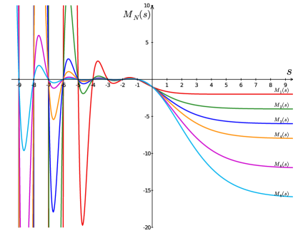
Equations (24) and (30) allow for some interesting analysis. The gamma function $\Gamma(x)$ has poles at $x=0,-1,-2,\ldots$ for which the Bessel sum in (24) and (30) vanishes. In this case we get

$$M_{N}(s)=-2\eta(2s)\quad{\rm if}~{}s=0,-1,-2,\ldots$$

(38)

which is independent of the dimension $N$. This implies that all Madelung curves cross at these critical points. Moreover, from the Dirichlet eta function we know that $\eta(2s)=0$ for $s=-1,-2,\ldots$. This behavior is nicely seen in Figure 7. Comparing with Zucker’s formulas we see that this is easily fulfilled for the specific dimensions given. Concerning the usual Madelung constant at $s=1/2$ we see that they lie close to the crossing point at $s=0$ which explains their rather slow decrease with increasing dimension $N$.

Zucker was able to evaluate the Madelung series analytically for even dimensions up to $N=8$ Zucker-1974 based on previous work of Glasser glasser1973 ; Glasser1973b . He further conjectured that $M_{3}(s)$ may be expressed in terms of a yet unknown Dirichlet series (for a recent analysis of lattice sums arising from the Poisson equation see Ref.Bailey_2013 ). Of considerable help for future investigations will be the condition that $M_{N}(0)=-1$ and $M_{N}(-n)=0$ for all $n\in\mathbb{N}$. At these critical points we have the following properties

	$\displaystyle\zeta(0)$	$\displaystyle=-\frac{1}{2}\quad,\quad\zeta(-2n)=0\quad,\quad\zeta(-n)=(-1)^{n}\frac{B_{n+1}}{n+1}$
	$\displaystyle\eta(0)$	$\displaystyle=\frac{1}{2}\quad,\quad\eta(-2n)=0\quad,\quad\eta(-n)=\frac{\left(2^{n+1}-1\right)}{n+1}B_{n+1}$		(39)
	$\displaystyle\beta(0)$	$\displaystyle=\frac{1}{2}\quad,\quad\beta(-2n+1)=0\quad,\quad\beta(-n)=\frac{E_{n}}{2}$

where $B_{n}$ and $E_{n}$ are the Bernoulli and Euler numbers respectively andrews1999special . For example, from Zucker’s formulas (10) and (11) we follow immediately that $M_{6}(0)=E_{2}=-1$ and $M_{8}(0)=2(2^{4}-1)B_{4}=-1$. Further, because of $\lim_{s\to\infty}\eta(s)=1$, $\lim_{s\to\infty}\beta(s)=1$, $\lim_{s\to\infty}\zeta(s)=1$ we see that the coefficients in front of the functions in eqs.(7)-(11) add up to exactly $-2N$. It is, however, incorrect to assume that analytical formulas in terms of these standard functions can be obtained for higher even dimensions. For a detailed discussion we refer to Appendix B. In this sense, our expansions in terms of Bessel functions is perhaps the closest general form for a fast convergent series we can get for the $N$-dimensional Madelung constant.

We presented fast convergent expressions for the Madelung constant in terms of Bessel function expansions which allow for an asymptotic exponential decay of the series. Even for higher dimensions the Madelung constants can be evaluated efficiently and accurately through the recursive expression or by using computer algebra to work with the generating functions. The number of representations of the $N$ sum of squares can also be efficiently handled through recursive relations. The Madelung constants and their analytical continuations can be calculated easily by standard mathematical software packages to any precision. These numbers may be useful for future explorations of analytical formulas in higher dimensions. For $s\geq 1/2$ a Fortran program with double precision accuracy is available from our CTCP website ProgramJones .

References

- (1) M. Born, A. Lande, Über die Berchnung der Kompressibilität regulärer Kristalle aus der Gittertheorie, Verhandl. d. dtsch. Phys. Ges. 20 (1918) 210.
- (2) M. Born, A. Lande, Über die absolute Berechnung der Kristalleigenschaften mit Hilfe Bohrscher Atommodelle, Ber. Preuss. Akad. Wiss. Berlin 45 (1918) 1048.
- (3) E. Madelung, Das elektrische Feld in Systemen von regelmäßig angeordneten Punktladungen, Phys. Z 19 (524) (1918) 32.
- (4) D. Quane, Crystal lattice energy and the madelung constant, J. Chem. Ed. 47 (5) (1970) 396.
-
(5)
O. Emersleben, Über die
Konvergenz der Reihen Epsteinscher Zetafunktionen. Erhard Schmidt
zum, 75. Geburtstag., Mathematische Nachrichten 4 (1-6) (1950) 468–480.
doi:10.1002/mana.3210040140.
URL http://dx.doi.org/10.1002/mana.3210040140 - (6) D. Borwein, J. Borwein, C. Pinner, Convergence of Madelung-like lattice sums, Trans. Am. Math. Soc. 350 (8) (1998) 3131–3167.
- (7) D. Borwein, J. M. Borwein, K. F. Taylor, Convergence of lattice sums and Madelung’s constant, J. Math. Phys. 26 (11) (1985) 2999–3009.
- (8) J. M. Borwein, M. Glasser, R. McPhedran, J. Wan, I. Zucker, Lattice sums then and now, no. 150, Cambridge University Press, 2013.
(9)
R. E. Crandall, J. P. Buhler,
Elementary function
expansions for Madelung constants, J.Phys. A: Math. Gen. 20 (16) (1987)
5497–5510.
doi:10.1088/0305-4470/20/16/024.
URL https://doi.org/10.1088/0305-4470/20/16/024 -
(10)
R. E. Crandall, New
representations for the madelung constant, Exper. Math. 8 (4) (1999)
367–379.
arXiv:https://doi.org/10.1080/10586458.1999.10504625, doi:10.1080/10586458.1999.10504625.
URL https://doi.org/10.1080/10586458.1999.10504625 -
(11)
S. Tyagi, New Series Representation
for the Madelung Constant, Prog. Theoret. Phys. 114 (3) (2005)
517–521.
arXiv:https://academic.oup.com/ptp/article-pdf/114/3/517/5161705/114-3-517.pdf,
doi:10.1143/PTP.114.517.
URL https://doi.org/10.1143/PTP.114.517 - (12) J. Zucker, Richard Crandall and the Madelung constant for salt, manuscript, at https://www.carma.newcastle.edu.au/resources/jon/LatticeSums/rec-madelung.pdf (2013).
- (13) G. Benson, A simple formula for evaluating the Madelung constant of a NaCl-type crystal, Can. J. Phys. 34 (8) (1956) 888–890.
- (14) J. Mackenzie, A simple formula for evaluating the Madelung constant of an NaCl-type crystal, Can. J. Phys. 35 (4) (1957) 500–501.
(15)
A. Hautot, New applications
of Poisson’s summation formula, J. Phys. A: Math. Gen. 8 (6) (1975) 853.
URL http://stacks.iop.org/0305-4470/8/i=6/a=004 -
(16)
P. Epstein, Zur Theorie
allgemeiner Zetafunktionen, Math. Ann. 56 (4) (1903) 615–644.
doi:10.1007/BF01444309.
URL http://dx.doi.org/10.1007/BF01444309 -
(17)
I. J. Zucker, Exact results
for some lattice sums in 2, 4, 6 and 8 dimensions, J.Phys. A: Math., Nucl.
Gen. 7 (13) (1974) 1568.
URL http://stacks.iop.org/0301-0015/7/i=13/a=011 - (18) G. Nebe, N. J. Sloane, A catalogue of lattices, Published electronically at http://www. research. att. com/njas/lattices (2012).
- (19) M. Mamode, Computation of the Madelung constant for hypercubic crystal structures in any dimension, J. Math. Chem. 55 (3) (2017) 734–751.
- (20) A. A. Terras, Bessel series expansions of the Epstein zeta function and the functional equation, Trans. Am. Math. Soc. 183 (1973) 477–486.
- (21) R. E. Crandall, Fast evaluation of Epstein zeta functions, manuscript, at https://www.reed.edu/physics/faculty/crandall/papers/epstein.pdf (1998).
(22)
A. Burrows, S. Cooper, E. Pahl, P. Schwerdtfeger,
Analytical methods for fast
converging lattice sums for cubic and hexagonal close-packed structures, J.
Math. Phys. 61 (12) (2020) 123503.
arXiv:https://doi.org/10.1063/5.0021159, doi:10.1063/5.0021159.
URL https://doi.org/10.1063/5.0021159 - (23) G. E. Andrews, R. Askey, R. Roy, Special functions, no. 71, Cambridge University Press, Cambridge, UK, 1999.
- (24) N. M. Temme, Special functions: An introduction to the classical functions of mathematical physics, John Wiley & Sons, New York, 1996.
- (25) G. Hardy, On the representation of a number as the sum of any number of squares, and in particular of five, Trans. Am. Math. Soc. 21 (3) (1920) 255–284.
- (26) R. A. Rankin, Sums of squares and cusp forms, Am. J. Math. 87 (4) (1965) 857–860.
- (27) J. Holley-Reid, J. Rouse, The number of representations of as a growing number of squares, arXiv preprint arXiv:1910.01001 (2019).
- (28) K. Ramachandra, Srinivasa Ramanujan (the inventor of the circle method)(22-12-1887 to 26-4-1920), Hardy-Ramanujan J. 10 (1987) 9–24.
- (29) M. L. Glasser, The evaluation of lattice sums. I. Analytic procedures, J. Math. Phys. 14 (3) (1973) 409–413.
(30)
M. L. Glasser, The evaluation of
lattice sums. II. Number‐theoretic approach, Journal of Mathematical
Physics 14 (6) (1973) 701–703.
arXiv:https://doi.org/10.1063/1.1666381, doi:10.1063/1.1666381.
URL https://doi.org/10.1063/1.1666381 -
(31)
D. H. Bailey, J. M. Borwein, R. E. Crandall, I. J. Zucker,
Lattice sums arising
from the Poisson equation, J. Phys. A: Math. Theoret. 46 (11) (2013)
115201.
doi:10.1088/1751-8113/46/11/115201.
URL https://doi.org/10.1088/1751-8113/46/11/115201 -
(32)
P. Schwerdtfeger, A. Burrows,
Program
Jones - A Fortran Program for Lattice Sums, Massey University, Auckland
(2022).
URL http://ctcp.massey.ac.nz/index.php?group=&page=fullerenes&menu=latticesums - (33) E. Artin, The gamma function, Courier Dover Publications, New York, 2015.
- (34) S. Cooper, Ramanujan’s theta functions, Springer, Berlin, 2017.
- (35) T. M. Apostol, Modular Functions and Dirichlet Series in Number Theory, Springer-Verlag New York, 1976.
- (36) S. Cooper, On sums of an even number of squares, and an even number of triangular numbers: an elementary approach based on Ramanujan’s summation formula, Contem. Math. 291 (2001) 115–138.