The Lanczos Approximation for the $\Gamma$-Function with Complex Coefficients

The $\Gamma$-function, defined by

$$\Gamma(z)=\int_{0}^{\infty}t^{z-1}e^{-t}dt$$

(1)

was introduced by Euler as a solution to the “interpolation” problem of defining the factorial function for non-integer values. Equation (1) has the desired property that $\Gamma(n+1)=n!$. The uniqueness of this definition was proved by Bohr and Mollerup (1922) and a second proof attributed to H. Wielandt is discussed by Remmert (1996) and included in the textbook by Freitag and Busam (2005),

In the form of Equation (1) it is defined in the complex plane for $\mathcal{R}e(z)>0$ and can be extended to the left half-plane, among other several other methods, through the use of the Euler reflection formula

$$\Gamma(z)\Gamma(1-z)=\frac{\pi}{\sin\pi z}.$$

(2)

The $\Gamma$-function has found wide application in pure and applied mathematics, statistics and the physical sciences. Exact values for the $\Gamma$-function can be found for positive integer (zero and the negative integers are simple poles) and for half integer values of $z$. Apart from those values, the $\Gamma$-function must be evaluated using numerical methods. To this end a number of approximations and asymptotic series have been developed. The earliest being Stirling’s approximation; for integer $n$

$$n!\approx\sqrt{2\pi n}n^{n}e^{-n}=\sqrt{2\pi n}\left(\frac{n}{e}\right)^{n}.$$

A large number of proofs of Stirling’s approximation and closely related formulas are available, see, for example, Aissen (1954), Feller (1967), Spira (1971), Namias (1986), Marsaglia and Marsaglia (1990), Deeba and Rodriguez (1991), Schuster (2001), Michel (2002), Dutkay et al. (2013), Lou (2014), and Neuschel (2014).

There are also a number of series expansions available such as Stirling’s asymptotic series

$$n!=\left(\frac{n}{e}\right)^{n}\sqrt{2\pi n}\exp\left(\frac{1}{12n}-\frac{1}{360n^{3}}+\frac{1}{1260n^{5}}-\dots\right).$$

There are some proofs which only require elementary methods such as that of Mermin (1984), Namias (1986), Diaconis and Freedman (1986), Patin (1989) and Marsaglia and Marsaglia (1990).

In addition there are series methods due to Spira (1971), Spouge (1994), and Schmelzer and Trefethen (2007). Among these other series Lanczos (1964) derived an expansion for the numerical evaluation of the $\Gamma$-function which was popularized to some extent by its inclusion in Press et al. (1997) and which was studied in some detail by Pugh (2004). The expansion has two notable features; it is convergent rather than an asymptotic expansion and it has a free parameter (denoted by $\gamma$ by Lanczos (1964) but by $r$ by Pugh (2004), we will use $r$ in this paper) which affects the rate of convergence of the approximation. While it is known that the free parameter can be complex, to the best of this author’s knowledge the convergence properties of a complex expansion have not been studied. Godfrey (2001) studied the convergence properties of the expansion for real values of $r$ and implemented his best choice of coefficients in Matlab (MATLAB, 2019) using 15 terms and giving an approximation that was accurate to 15 significant digits along the real axis and 13 significant digits elsewhere.

The Lanczos expansion,, which is for $\Gamma(z+1)$ rather than $\Gamma(z)$, can be written

$$\Gamma(z+1)=\sqrt{2\pi}\left(z+r+\frac{1}{2}\right)^{z+\frac{1}{2}}e^{-\left(z+r+\frac{1}{2}\right)}\\ \left[\frac{a_{0}(r)}{2}+\frac{z}{z+1}a_{1}(r)+\frac{(z-1)z}{(z+2)(z+1)}a_{2}(r)+\cdots\right]$$

(3)

where the $a_{k}(r)$ are the coefficients and $r$ is the free parameter.

The key to obtaining the $a_{k}(r)$ is to note that the $\Gamma$-function has known values at the integers and that for positive integers the expansion (3) terminates, allowing the $a_{k}(r)$ to be determined recursively. Pugh (2004) investigated several methods of obtaining the $a_{k}(r)$ and reported the recursive methods worked well in practice.

In (3) if $z=0$ then $\Gamma(1)=1$ and the series terminates after the first term. Thus

	$\displaystyle 1$	$\displaystyle=\sqrt{2\pi}\left(r+\frac{1}{2}\right)^{1/2}e^{-\left(r+\frac{1}{2}\right)}\frac{a_{0}(r)}{2}.$
Solving for $a_{0}(r)$ we obtain
	$\displaystyle a_{0}(r)$	$\displaystyle=\sqrt{\frac{2e}{\pi(r+\frac{1}{2})}}e^{r}.$		(4)

Having obtained $a_{0}(r)$ we then set $z=1$ so that $\Gamma(2)=1$ and (3) now terminates after the second term allowing us to find $a_{1}(r)$. By successively setting $z=2,3,4\ldots$ we can calculate as many of the $a_{k}(r)$ as required.

On a practical matter of finding the $a_{k}(r)$ it is useful to set

	$\displaystyle F_{r}(z)$	$\displaystyle=\frac{\Gamma(z+1)e^{z+r+1/2}}{\sqrt{2\pi}\left(z+r+1/2\right)^{z+1/2}}.$		(5)
Then
	$\displaystyle a_{1}$	$\displaystyle=\left(F_{r}(1)-\frac{a_{0}}{2}\right)\frac{2}{1}$		(6)
	$\displaystyle a_{2}$	$\displaystyle=\left(\left(F_{r}(2)-\frac{a_{0}}{2}\right)\frac{3}{2}-a_{1}\right)\frac{4}{1}$		(7)
The general ($n\geq 3$) recursion formula is
	$\displaystyle a_{n}(r)$	$\displaystyle=\left(\left(\left(\left(F_{r}(n)-\frac{a_{0}}{2}\right)\frac{n+1}{n}-a_{1}\right)\frac{n+2}{n-1}-a_{2}\right)\frac{n+3}{n-2}-\cdots-a_{n-1}\right)\frac{2n}{1}.$		(8)

The final equation is Pugh (2004) Equation (6.4).

Having found some $a_{k}(r)$ values they are substituted into the expansion (3) and desired approximations of $\Gamma(z+1)$ can be obtained, values with $\mathcal{R}e(z)<0$ can be obtained by combining the Lanczos approximation with the Euler reflection formula, Equation (2).

In the remainder of this paper Section (2) investigates some of the properties of the Lanczos coefficients with complex values of the free parameter, Section (3) reports on the numerical performance of series with complex coefficients, Section (4) presents our conclusions while Appendix (A) presents some supplementary materials.

The formulas (4) through (8) allow us to calculate the expansion coefficients with complex $r$. All numerical values and graphics presented here were obtained with custom written Matlab (MATLAB, 2019) code. The code was verified using published values of the $a_{k}(r)$ for real $r$ in Lanczos (1964) and Pugh (2004) and then, without any further alteration of the code, $r$ was allowed to be complex and the required coefficients calculated.

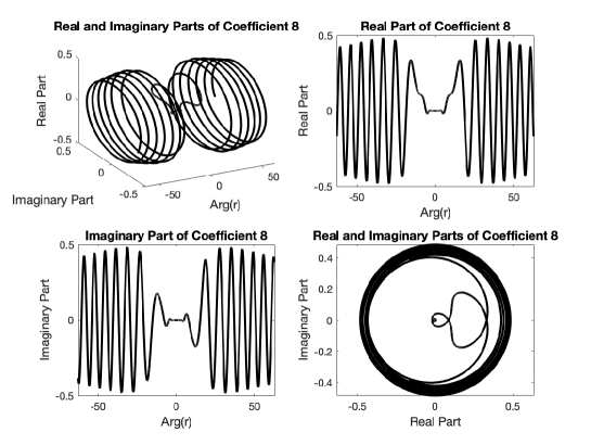
Figures (1) through (5) present five different views of the $a_{0}(r)$ coefficient for $r=1+ir_{y}$ with $-20\pi\leq r_{y}\leq 20\pi$. While we explored values of $r$ with different real parts ($\mathcal{R}e(r)=1,3,\ldots,13$), the behaviour of the coefficients were similar in all cases, the main change being their magnitudes.

In the recursive calculation of the $a_{k}(r)$ only integer values of $z$ are used so we denote these by $n=1,2,3,\ldots$. The free parameter enters at two points. In the numerator of the $F_{r}(z)$, Equation (5), with $n=1,2,3,\ldots$, has the term $e^{n+r+1/2}$. Writing $r=r_{x}+ir_{y}$ the real part of the exponent is $n+r_{x}+1/2$ while the imaginary part is $ir_{y}$. Holding the real part constant and allowing $\mathcal{I}m(r)$ to change makes the coefficients “spin” in the complex plane, examples can be seen in Figures (1), (4) and (5).

The other place $r$ enters the calculation of the $a_{k}(r)$ is in the denominator of $F_{r}(z)$. This is what causes the “tappering off” seen in Figure (1) through (3) and the gradual descent of the path of the $a_{k}(r)$ on the Riemann sphere, see Figure (5). If

	$\displaystyle r$	$\displaystyle=r_{x}+ir_{y}$
We can rewrite this in polar form
	$\displaystyle r$	$\displaystyle=Re^{i\theta}$
where
	$\displaystyle R$	$\displaystyle=\sqrt{r_{x}^{2}+r_{y}^{2}}$
	$\displaystyle\theta$	$\displaystyle=\tan^{-1}\left(\frac{r_{y}}{r_{x}}\right).$

If $r_{x}$ is fixed increasing $|r_{y}|$ increases $R$ causing the tapper. Asympotitically the real and imaginary parts of $a_{0}(r)$ decay as $1/\sqrt{r_{y}}$.

Figures (2) and (3) suggest that there are points for fixed $r_{x}$ ($r_{x}=1$ in the Figures) for which the $a_{0}(r)$ will be purely real or purely imaginary. We can derive conditions under which these cases occur and show that there are an infinite number of such coefficients.

Using Equation (4), if $a_{0}(r)$ is purely imaginary then it has the form $a_{0}(r)=iv$. Thus

	$\displaystyle iv$	$\displaystyle=\sqrt{\frac{2e}{\pi(r+\frac{1}{2})}}e^{r}$
	$\displaystyle-v^{2}$	$\displaystyle=\frac{2e}{\pi(r+\frac{1}{2})}e^{2r}.$
First, splitting $r$ into its real and imaginary parts we have
	$\displaystyle-v^{2}$	$\displaystyle=\frac{2e}{\pi\left((r_{x}+\frac{1}{2})+ir_{y}\right)}e^{2r_{x}+i2r_{y}}.$
Next, we proceed to split this into its real and imaginary parts
	$\displaystyle-v^{2}$	$\displaystyle=\frac{2e^{2r_{x}+1}}{\pi\left(\left(r_{x}+\frac{1}{2}\right)^{2}+r_{y}^{2}\right)}\left(\left(r_{x}+\frac{1}{2}\right)-ir_{y}\right)\left(\cos 2r_{y}+i\sin 2r_{y}\right)$

Thus we have

$$-v^{2}=\frac{2e^{2r_{x}+1}}{\pi\left(\left(r_{x}+\frac{1}{2}\right)^{2}+r_{y}^{2}\right)}\Bigg{[}\left(\left(r_{x}+\frac{1}{2}\right)\cos 2r_{y}+r_{y}\sin 2r_{y}\right)\\ +i\left(\left(r_{x}+\frac{1}{2}\right)\sin 2r_{y}-r_{y}\cos 2r_{y}\right)\Bigg{]}.$$

From this we neglect the sign of the leading fraction because it is always positive. This leaves us with two conditions for the $a_{0}(r)$ to be purely imaginary. The first is that real part must be negative, that is

	$\displaystyle\left(r_{x}+\frac{1}{2}\right)\cos 2r_{y}+r_{y}\sin 2r_{y}$	$\displaystyle<0$
or
	$\displaystyle\tan 2r_{y}<-\frac{r_{x}+1/2}{r_{y}}.$			(9)
Secondly, we require that the imaginary part is zero
	$\displaystyle\left(r_{x}+\frac{1}{2}\right)\sin 2r_{y}-r_{y}\cos 2r_{y}$	$\displaystyle=0.$
From this second condition we require
	$\displaystyle\tan 2r_{y}$	$\displaystyle=\frac{r_{y}}{r_{x}+1/2}.$		(10)
For the $a_{0}(r)$ to be purely real the condition on the imaginary part (Equation 10) is unchanged and in place of Equation (9) we require
	$\displaystyle\left(r_{x}+\frac{1}{2}\right)\cos 2r_{y}+r_{y}\sin 2r_{y}$	$\displaystyle>0.$
or
	$\displaystyle\tan 2r_{y}<-\frac{r_{x}+1/2}{r_{y}}.$			(11)

Pragmatically, to find the values of $r$ for which the $a_{0}(r)$ are purely real or imaginary requires solving Equation (10) numerically and then checking the conditions in Equations (9) and (11).

It is obvious that using a Lanczos approximation with complex $r$ increases the computational cost of calculating the $\Gamma$-function when the same number of coefficients are used. Thus to use complex coefficients requires a compelling case that there are significant advantages in the convergence rate and/or accuracy of the approximation compared to real coefficients. In this section we examine whether such a case can be made.

In all cases we used 10 coefficients in the approximation. Figures (8) through (11) present the results, we discuss how the data in each Figure was generated and comment on its significance.

We generated 13 sets of 10 coefficients using the recursive method described above by setting $r=1+in\pi/6$ where $n=0,1,\ldots,12$. In Figures (8) and (9) the imaginary part of $r$ is presented on the axis label $Im(r)$. We generated 22 values of $z+1=1.5,2.0,2.5,\ldots,12$ for which exact values could be calculated. These were obtained for integer values from the factorial property, namely $\Gamma(n+1)=n!$ and for half integer values from the functional equation

$$\Gamma(z+1)=z\Gamma(z)$$

coupled with the value $\Gamma(1/2)=\sqrt{\pi}$.

Figure (8) presents the absolute value of the error while Figure (9) presents the relative error, that is the absoluate error is divided by the exact value. In both cases it is clear that the Lanczos coefficients generated by real $r$ performed better. The absolute error is never large (less than 3 for $11!\approx 3.9\times 10^{7}$ but largest error occurs for coefficients generated with $r=1+i2\pi$.

The relative error presented in Figure (9) is more informative. The vertical axis is truncated at an error of $10^{-7}$ in order to better see the relative error at the half-integer values.. It clear that in all cases the relative error is indistiquishable from zero for integer values up to $z+1=10$ for all values of$r$. This is because they were used to generate the coefficients. However, the half integer values of $z+1$ show increasing relative errors as the imaginary part increases from $0$ to $2\pi$. Somewhat similar, once we progress beyond the integer values of $z+1$ which we used to generate the coefficients, i.e. $z+1=10$, the relative error builds rapidly with increasing imaginary part of $r$. At least on the scale used in the Figure the relative error for the coefficients are indistinquiable from zero for real $r$.

For Figures (10) and (11), using the same coefficients as above, we considered the performance of the approxmation for complex values of $z+1$. We set $z+1=6+n\pi i/12$ for $n=0,1,\ldots,24$. To find comparison values we used the Godfrey (2001) implementation discussed above. For both the absolute and relative error cases, the Lanczos approximation performance deteriorated as the imaginary part of $z+1$ increased and as the imaginary part of $r$ increased together.

Figure (6) suggests that as the imagary part of $r$ increases all coefficients converge to the same magnitude. For the coefficients displayed in Figure (7), i.e. for $r=1+20\pi i$, we tested its performance against the Godfrey (2001) implementation. We do not present detailed results here, suffice to say that as the imaginary part of $z+1$ increased the relative error increased very rapidly.

We explored the possibility that complex values of the free parameter $r$ in the Lanczos (1964) approximation for the $\Gamma$-function could improve the rate of convergence of the approximation. However, we must conclude that there is no advantage to using complex values of $r$, in fact, it appears uniformly detrimental. The real values of $r$ for the values we explored uniformly gave the lowest relative error when compared with exact values of the $\Gamma$-function at integer and half integer values. Further, Lanczos coefficients generated by real values of $r$ also uniformly gave the lowest relative error for complex values of the $z$ in $\Gamma(z+1)$.

Unless there are purely mathematical reasons for further studying the properties of complex Lanczos coefficients they appears to be a dead end in applied numerical analysis.

References

- Aissen (1954) Aissen, M. I. (1954). Some Remarks on Stirling’s Formula. The American Mathematical Monthly 61(10), 687–691.
- Bohr and Mollerup (1922) Bohr, H. and J. Mollerup (1922). Laereborg i Matematisk Analyse, Volume III. J. Gjellerup, Kopenhagen.
- Deeba and Rodriguez (1991) Deeba, E. Y. and D. M. Rodriguez (1991). Stirling’s Series and Bernoulli Numbers. The American Mathematical Monthly 98(5), 423–326.
- Diaconis and Freedman (1986) Diaconis, P. and D. Freedman (1986). An Elementary Proof of Stirling’s Formula. The American Mathematical Monthly 93(2), 123–125.
- Dutkay et al. (2013) Dutkay, D. E., C. P. Niculescu, and F. Popovici (2013). Stirling’s Formula and its Extension for the Gamma Function. The American Mathematical Monthly 120(8), 737–740.
- Feller (1967) Feller, W. (1967). A Direct Proof of Stirling’s Formula. The American Mathematical Monthly 74(10), 1223–1225.
- Freitag and Busam (2005) Freitag, E. and R. Busam (2005). Complex Analysis. Springer.
- Godfrey (2001) Godfrey, P. (2001). A Note on the Computation of the Convergent Lanczos Complex Gamma Approximations. http://my.fit.edu/ gabdo/paulbio.html.
- Lanczos (1964) Lanczos, C. (1964). A Precision Approximation of the Gamma Function. Journal of the Society for Industrial and Applied Mathematics: Series B, Numerical Analysis 1, 86–96.
- Lou (2014) Lou, H. (2014). A Short Proof of Stirling’s Formula. The American Mathematical Monthly 121(2), 154–157.
- Marsaglia and Marsaglia (1990) Marsaglia, G. and J. C. W. Marsaglia (1990). A New Derivation of Stirling’s Approximation to n! The American Mathematical Monthly 97(9), 826–829.
- MATLAB (2019) MATLAB (2019). version 9.6.0.1072779 (R2019a). Natick, Massachusetts: The MathWorks Inc.
- Mermin (1984) Mermin, N. D. (1984). Stirling’s formula! American Journal of Physics 52(4), 362–365.
- Michel (2002) Michel, R. (2002). On Stirling’s Formula. The American Mathematical Monthly 109(4), 388–390.
- Namias (1986) Namias, V. (1986). A Simple Derivation of Stirling’s Asymptotic Series! The American Mathematical Monthly 93(1), 25–29.
- Neuschel (2014) Neuschel, T. (2014). A New Proof of Stirling’s Formula. The American Mathematical Monthly 121(4), 350–352.
- Patin (1989) Patin, J. M. (1989). A Very Short Proof of Stirling’s Formula. The American Mathematical Monthly 96(1), 41–42.
- Press et al. (1997) Press, W. H., S. A. Teukolsky, W. T. Vetterling, and B. P. Flannery (1997). Numerical Recipes. Cambridge University Press.
- Pugh (2004) Pugh, G. R. (2004). An Analysis of the Lanczos Gamma Approximation. Ph.D. Thesis, The University of British Columbia.
- Remmert (1996) Remmert, R. (1996). Wielandt’s Theorem About the -Function. The American Mathematical Monthly 103(3), 214–220.
- Schmelzer and Trefethen (2007) Schmelzer, T. and L. N. Trefethen (2007). Computing the Gamma Function Using Contour Integrals and Rational Approximations. SIAM Journal on Numerical Analysis 45(2), 558–571.
- Schuster (2001) Schuster, W. (2001). Improving Stirling’s Formula. Archiv der Mathematik 77, 170–176.
- Spira (1971) Spira, R. (1971). Calculation of the Gamma Function by Stirling’s Formula. Mathematics of Computation 25(114), 317–322.
- Spouge (1994) Spouge, J. L. (1994). Computation of the Gamma, Digamma and Trigamma Functions. SIAM Journal on Numerical Analysis 31(3), 931–944.
Appendix A Plots of Coefficients 0 through 10
A.1 Real and Imaginary Parts of the Coefficients
A.2 Coefficients on the Riemann Sphere
A.3 Magntitudes of the Coefficients