The Kinematics, Metallicities, and Orbits of Six Recently Discovered Galactic Star Clusters with Magellan/M2FS Spectroscopy^†^†thanks: This paper presents data gathered with the Magellan Telescopes at Las Campanas Observatory, Chile.

Andrew B. Pace,¹ Sergey E. Koposov,^2,3,4,1 Matthew G. Walker,¹ Nelson Caldwell,⁵ Mario Mateo, ⁶ Edward W. Olszewski, ⁷ Ian U. Roederer, ^6,8 John I. Bailey, III, ⁹ Vasily Belokurov,³ Kyler Kuehn, ¹⁰ Ting S. Li, ¹¹ Daniel B. Zucker ^12,13
¹McWilliams Center for Cosmology, Carnegie Mellon University, 5000 Forbes Ave, Pittsburgh, PA 15213, USA
²Institute for Astronomy, University of Edinburgh, Royal Observatory, Blackford Hill, Edinburgh EH9 3HJ, UK
³Institute of Astronomy, University of Cambridge, Madingley Road, Cambridge CB3 0HA, UK
⁴Kavli Institute for Cosmology, University of Cambridge, Madingley Road, Cambridge CB3 0HA, UK
⁵Harvard-Smithsonian Center for Astrophysics, 60 Garden Street, MS-15, Cambridge, MA 02138, USA
⁶Department of Astronomy, University of Michigan, Ann Arbor, MI 48109, USA
⁷Steward Observatory, The University of Arizona, 933 N. Cherry Avenue, Tucson, AZ 85721, USA
⁸Joint Institute for Nuclear Astrophysics – Center for the Evolution of the Elements (JINA-CEE), USA
⁹Department of Physics, UCSB, Santa Barbara, CA 93016, USA
¹⁰ Lowell Observatory, 1400 W Mars Hill Rd, Flagstaff, AZ 86001, USA
¹¹Department of Astronomy and Astrophysics, University of Toronto, 50 St. George Street, Toronto ON, M5S 3H4, Canada
¹² School of Mathematical and Physical Sciences, Macquarie University, Sydney, NSW 2109, Australia
¹³ Macquarie University Research Centre for Astronomy, Astrophysics & Astrophotonics, Sydney, NSW 2109, Australia
E-mail: [email protected]

(Accepted XXX. Received YYY; in original form ZZZ)

Abstract

We present Magellan/M2FS spectroscopy of four recently discovered Milky Way star clusters (Gran 3/Patchick 125, Gran 4, Garro 01, LP 866) and two newly discovered open clusters (Gaia 9, Gaia 10) at low Galactic latitudes. We measure line-of-sight velocities and stellar parameters ([Fe/H], $\log{g}$ , $T_{\rm eff}$ , [Mg/Fe]) from high resolution spectroscopy centered on the Mg triplet and identify 20-80 members per star cluster. We determine the kinematics and chemical properties of each cluster and measure the systemic proper motion and orbital properties by utilizing Gaia astrometry. We find Gran 3 to be an old, metal-poor (mean metallicity of ${\rm[Fe/H]}=-1.83$ ) globular cluster located in the Galactic bulge on a retrograde orbit. Gran 4 is an old, metal-poor ( ${\rm[Fe/H]}=-1.84$ ) globular cluster with a halo-like orbit that happens to be passing through the Galactic plane. The orbital properties of Gran 4 are consistent with the proposed LMS-1/Wukong and/or Helmi streams merger events. Garro 01 is metal-rich ( ${\rm[Fe/H]}=-0.30$ ) and on a near circular orbit in the outer disk but its classification as an open cluster or globular cluster is ambiguous. Gaia 9 and Gaia 10 are among the most distant known open clusters at $R_{GC}\sim 18,~{}21.2~{}\mathrm{\,kpc}$ and most metal-poor with [Fe/H] $\sim-0.50,-0.34$ for Gaia 9 and Gaia 10, respectively. LP 866 is a nearby, metal-rich open cluster ([Fe/H] $=+0.10$ ). The discovery and confirmation of multiple star clusters in the Galactic plane shows the power of Gaia astrometry and the star cluster census remains incomplete.

keywords:

Stars: kinematics and dynamics – globular clusters: general – open clusters and associations: general

^†^†pubyear: 2023^†^†pagerange: The Kinematics, Metallicities, and Orbits of Six Recently Discovered Galactic Star Clusters with Magellan/M2FS Spectroscopy^†^†thanks: This paper presents data gathered with the Magellan Telescopes at Las Campanas Observatory, Chile.– The Kinematics, Metallicities, and Orbits of Six Recently Discovered Galactic Star Clusters with Magellan/M2FS Spectroscopy^†^†thanks: This paper presents data gathered with the Magellan Telescopes at Las Campanas Observatory, Chile.

1 Introduction

Star clusters are among the smallest stellar structures in the universe and are a key component of hierarchical structure assembly. They are valuable for studying stellar populations and their evolution at a variety of ages, metallicities, and environs (e.g., Krumholz et al., 2019; Adamo et al., 2020). Star clusters in the Milky Way (MW) are typically divided into two categories: the older, denser, and more luminous globular clusters (Gratton et al., 2019), and the younger clusters in the MW disk, referred to as open clusters (e.g., Cantat-Gaudin, 2022).

While the census of bright halo clusters is mostly complete (Webb & Carlberg, 2021), there has been a number of faint star clusters discovered in optical wide-field imaging surveys, pushing the luminosity and surface brightness boundary (e.g, Koposov et al., 2007; Belokurov et al., 2014; Torrealba et al., 2019; Mau et al., 2019; Cerny et al., 2023). The census of star clusters in the MW mid-plane is incomplete due to the high extinction and large stellar foreground. With recent near-infrared surveys such as the VISTA Variables in the Via Láctea Survey (VVV) (e.g., Minniti et al., 2011; Garro et al., 2020) and astrometric data from the Gaia mission the number of star cluster candidates has significantly increased (e.g., Koposov et al., 2017; Torrealba et al., 2019; Garro et al., 2020; Gran et al., 2022). However, a number of the star cluster candidates found pre-Gaia DR2 have been shown to be false positives once proper motions and kinematics are considered (Gran et al., 2019; Cantat-Gaudin & Anders, 2020).

Ultimately, stellar spectroscopy is required to validate candidate star clusters and confirm they are not a mirage of MW stars (e.g., Gran et al., 2022). Furthermore, spectroscopic radial velocities and metallicities will identify star cluster members. With the systemic radial velocity, the orbit and origin of a star cluster can be determined (e.g., Massari et al., 2019; Kruijssen et al., 2019)and the internal dynamics analyzed with large radial velocity samples (e.g., Baumgardt & Hilker, 2018; Garro et al., 2023). Spectroscopic metallicities can assist in determining the classification and origin of a star cluster (e.g., Gran et al., 2022).

We present spectroscopic confirmation of three recently discovered globular cluster candidates (Gran 3, Gran 4, Garro 01) and three newly discovered open clusters (Gaia 9, Gaia 10, LP 866). In Section 2, we discuss our search algorithm and independent discovery of the star cluster candidates with Gaia DR2. In Section 3, we discuss our spectroscopic observations, velocity and metallicity measurements, and the auxiliary data analyzed. In Section 4, we identify members of each star cluster, measure the general kinematic and metallicity properties, measure the spatial distribution, and determine the orbital properties. In Section 5, we analyze the globular cluster internal kinematics, compare the globular clusters to other MW globular clusters, discuss the origin and potential association to accretion events, analyze the open clusters in the context of the Galactic metallicity gradient, and compare our results to the literature. We summarize our conclusions in Section 6.

2 Discovery and Candidate identification

The search for the stellar overdensities was carried out in 2018 after the release of the Gaia DR2 using the satellite detection pipeline broadly based on the methods presented in Koposov et al. (2008); Koposov et al. (2015), but extended into space of proper motions.

We describe here briefly the basics behind the detection algorithm, leaving a more detailed description to a separate contribution (Koposov et al. in prep.).

The algorithm consists of several steps.

•

Looping over all proper motions. In the search used here we ran overdensity search for subsets of stars with proper motions $|\mu_{\alpha}-X_{i}|<1$ , $|\mu_{\delta}-X_{j}|<1$ where $X_{i}$ , $X_{j}$ span the range of proper motions from -15 to 15 mas/year with 1 mas/year steps.
•

Looping over all possible distance moduli to overdensities. We perform the search for stars selected based on an isochrone filter placed at distances from $\sim$ 6 kpc to 160 kpc. We used the extinction corrected BP, RP and G magnitudes and an old metal-poor PARSEC isochrone (Bressan et al., 2012) with an age of 12 Gyr and $[{\rm Fe/H}]=-2$ . We also run a single search without any isochrone colour magnitude selection.
•

Looping over overdensity sizes from 3 arcmin to 48 arcmin.
•

Segmentation of the sky into HEALPIX (Górski et al., 2011) tiles. To avoid having to work with the dataset for the entire sky the overdensity search algorithm works with approximately rectangular-shaped HEALPIX tiles, that we also increase in size by 20% with respect to the standard HEALPIX scheme to ensure overlap between tiles and avoid dealing with edge effects. The exact Nside resolution parameter and pixel scale of tiling were different for different runs depending on memory limitations and size of the overdensity being searched for.
•

Creation of a pixelated stellar density map inside each tile. We use tangential projection to map the stars into a rectangular x,y pixel grid, and then make a 2-D histogram of stellar counts of stars selected by proper motions, colours and magnitudes.
•

Creation of a stellar overdensity significance map based on a stellar count map. This step is described below in more detail.
•

Identification of overdensities based on the significance map and merging of candidate lists from various search configurations.
•

Cross-matching the candidate lists with external catalogues and construction of validation plots.

Below we provide a brief description of the algorithm that provides an overdensity significance map given the binned 2D stellar density map. The algorithm requires three main parameters – the kernel size, which corresponds to the size of the overdensity $k$ we are looking for, and two background apertures, $b_{1}$ and $b_{2}$ . Here we assume that we have a rectangular grid of stellar number counts $H(x,y)$ and we estimate the significance of the overdensity at pixel x=0, y=0. The key difference of our approach compared to previous approaches (i.e., Koposov et al., 2008) is that we do not rely on the assumption of Gaussianity or even a Poisson distribution of number counts in the map.

We first compute the number of stars $N$ in a circular aperture with radius k around the pixel 0,0. We then need to characterize what is the probability distribution of $P_{null}(N)$ under a null hypothesis of no overdensity to compute the tail probability/significance.

Our model for $P_{null}(N)$ is the negative-binomial distribution, which is a discrete Poisson-like distribution (that is, an infinite mixture of Poisson distributions with means having a Gamma distribution). The negative binomial distribution can be parameterized with mean $\mu$ and $\sigma^{2}$ , where $\sigma^{2}\geq\mu$ (note that the variance of the negative-binomial distribution is a parameter, as opposed to a Poisson distribution, where it is equal to the mean). The $\mu$ and $\sigma$ are estimated based on the number count distribution between two background apertures $b_{1}$ and $b_{2}$ .

The significance (or the Z-score) in each pixel is then assigned as $Z=F^{-1}(P_{null}(\geq N))$ , where $F^{-1}()$ is the inverse of the CDF of a normal distribution. The significant overdensities are selected as those where Z is larger than a certain threshold. For this work we used $Z>6$ selected candidates.

The application of the algorithm summarized above to Gaia DR2 in 2018 yielded a few hundred significant distinct overdensities. The absolute majority of them were known, but around 30 objects were deemed to be likely real dwarf galaxies or globular clusters and were selected for further inspection. The spectroscopic follow-up of six of these objects is the subject of this paper. Some objects from the list, such as the Eridanus IV object (Cerny et al., 2021) have been discovered and independently followed up since.

We began our spectroscopic follow-up in 2018 and note that 4 star clusters in our sample have since been independently discovered. We refer to these clusters by their name in the first discovery analysis. Garro 01 was independently discovered by Garro et al. (2020) in the near-IR VISTA Variables in the Via Láctea Extended Survey (VVVX). Gran et al. (2022) independently discovered Gran 3 (also known as Patchick 125) and Gran 4 with Gaia DR2 astrometry, and they were confirmed with the VVV survey. Gran 3 was independently discovered by the amateur astronomer Dana Patchick and named Patchick 125. We used the literature open cluster compilation from Hunt & Reffert (2023) to search for literature cross matches for our open clusters which includes most post-Gaia open cluster discoveries (e.g., Bica et al., 2019; Liu & Pang, 2019; Cantat-Gaudin & Anders, 2020; Kounkel et al., 2020; Castro-Ginard et al., 2022). One cluster, internally KGO 8, was independently discovered by Liu & Pang (2019) and referred to as LP 866 (although in some catalogs it is referred to as FoF 866) and Kounkel et al. (2020) and referred to as Theia 4124. We refer to this open cluster as LP 866 here. The two remaining open clusters in our sample are new discoveries, and we name them Gaia 9 and Gaia 10.

3 Spectroscopic Follow-Up

Table 1: Spectroscopic Observations of Star Clusters.

object	R.A. (deg)	Dec. (deg)	Telescope/Instrument	UT Date	Exp. Time	$N_{\mathrm{obs}}$	$N_{\mathrm{good}}$
Gran 3	$256.135833$	$-35.471278$	Magellan/M2FS	2018-08-11	6900	54	41
Gran 4	$278.092083$	$-23.211194$	Magellan/M2FS	2018-08-13	6100	118	115
Gran 4	$278.112121$	$-23.103756$	AAT/AAOmega	2018-06-24	1800	67	67
Garro 01	$212.246250$	$-65.738333$	Magellan/M2FS	2018-08-11	5400	205	193
Gaia 9	$119.607083$	$-38.984639$	Magellan/M2FS	2018-12-06	5400	96	50
Gaia 10	$121.172500$	$-38.984444$	Magellan/M2FS	2018-08-15	5800	56	43
LP 866	$261.651250$	$-39.280889$	Magellan/M2FS	2018-12-05	7200	164	160

3.1 Spectroscopic targeting

The possible member stars from candidate stellar overdensities discovered were selected for spectroscopic observations by using the information about the objects that was available from their detection, such as approximate object angular size and proper motion. We did not have a uniform target selection strategy from object to object, so we provide a broad overview of the selection. We typically targeted stars using Gaia DR2 astrometry and photometry, selecting stars with proper motions within 1-3 mas/yr of the center of the detection. We applied the astrometric_excess_noise <1 cut and selected stars with small parallaxes $\varpi<{\rm Max}(0.1,3\,\sigma_{\varpi})$ . Since the majority of followed-up overdensities had small angular sizes we tried to maximise the number of fibers on each object by assigning higher priority to central targets. We also did not apply any colour-magnitude or isochrone selection masks to the targets, other than a magnitude limit to ensure sufficient signal to noise, and prioritising brighter stars, such as $G<16-18$ .

3.2 M2FS Spectroscopy

We present spectroscopic observations of six star cluster candidates that we obtained using the Michigan/Magellan Fiber System (M2FS; Mateo et al., 2012) at the 6.5-m Magellan/Clay Telescope at Las Campanas Observatory, Chile. M2FS deploys 256 fibers over a field of diameter $0.5^{\circ}$ , feeding two independent spectrographs that offer various modes of configuration. We used both spectrographs in identical configurations that provide resolving power $\mathcal{R}\sim 24,000$ over the spectral range $5130-5190$ Å. For all six clusters, Table 1 lists coordinates of the M2FS field center, UT date and exposure time of the observation, the number of science targets and the number that yielded ‘good’ observations that pass our quality-control criteria.

We process and model all M2FS spectra using the procedures described in detail by Walker et al. (2023). Briefly, we use custom Python-based software to execute standard processing steps (e.g., overscan, bias and dark corrections), to identify and trace spectral apertures, to extract 1D spectra, to calibrate wavelengths, to correct for variations in pixel sensitivity and fiber throughput, and finally to subtract the mean sky level measured from $\sim 20$ fibers per field that are pointed toward regions of blank sky. To each individually-processed spectrum, we fit a model based on a library of synthetic template spectra computed on a regular grid of stellar-atmospheric parameters: effective temperature ( $T_{\rm eff}$ ), surface gravity ( $\log g$ ), metallicity ([Fe/H]) and magnesium abundance ([Mg/Fe]). Including parameters that adjust the resolution and continuum level of the template spectra, our spectral model has 16 free parameters. We use the software package MultiNest to draw random samples from the 16-dimensional posterior probability distribution function (PDF) (Feroz & Hobson, 2008; Feroz et al., 2009). We summarize 1D posterior PDFs for each of the physical parameters according to the mean and standard deviation of the sample returned by MultiNest.

We consider stars with ${\rm S/N}>0$ and $\sigma_{v_{\rm los}}>5\mathrm{\,km}\mathrm{\,s}^{-1}$ as good quality measurements (Walker et al., 2023). We consider stars with ${\rm S/N}>2$ to be good quality [Fe/H] measurements. Our selection of cuts for good quality [Fe/H] is based on repeat measurements and dwarf galaxy data in the M2FS catalog (Walker et al., 2023).

3.3 AAT Observations

One of the objects detected in the Gaia search was submitted for follow-up observations by the Two-degree Field (2dF) spectrograph (Lewis et al., 2002) at the Anglo-Australian Telescope (AAT). The observations were conducted during the observing run of the Southern Stellar Stream Spectroscopic Survey ( $S^{5}$ ) (Li et al., 2019). In particular, an internal data release (iDR3.1) was used for this work. We refer to Li et al. (2022) for a detailed description of the data and processing and provide a brief summary here. The stars were observed with two arms of the spectrograph: the red arm with the 1700D grating that covers a wavelength range from 8400 to 8800 Å (including Ca ii near-infrared triplet with $\lambda\lambda$ 8498, 8542, and 8662) with a spectral resolution of $R\sim 10000$ , and the blue arm with the 580V grating that provides low resolution $R\sim 1300$ spectra covering a broad wavelength range from 3800 to 5800 Å. The blue and red spectra for each star were then forward modeled by the rvspecfit code (Koposov, 2019) to provide estimates of stellar parameters, radial velocities and their uncertainties. In addition to the velocities, we also acquired the calcium triplet (CaT) metallicities from equivalent widths and the Carrera et al. (2013) calibration for all the member stars as detailed in Li et al. (2022).

3.4 Additional Data

We use photometric and astrometric data from the Gaia EDR3 catalog (Gaia Collaboration et al., 2021). We only utilize astrometric data that passed the following cuts: ruwe $<1.5$ (Lindegren et al., 2021), and astrometric_excess_noise_sig $<3$ . We note that some stars that were targeted spectroscopically do not pass these quality cuts (partly due to the Gaia DR2 target selection) and we exclude those stars from any astrometry based analysis. For parallax measurements, we apply the parallax offset from Lindegren et al. (2021) and include an additional offset of $\Delta\varpi=0.007~{}{\rm mas}$ based on the globular cluster analysis of Vasiliev & Baumgardt (2021).

We use Gaia DR3 RR Lyrae (RRL) catalog to search for candidate RRL star cluster members (Clementini et al., 2022). We use the DECam Plane Survey (DECaPS) DR1 griz photometric data for Gran 3, Garro 01 and LP 866 (Schlafly et al., 2018). We search for additional spectroscopic members of our star cluster sample in large spectroscopic surveys including SDSS APOGEE DR17 (Abdurro’uf et al., 2022), GALAH (Buder et al., 2021), and Gaia RVS DR3 (Katz et al., 2022).

4 Results

Table 2: Properties of the Star Clusters. Literature

M_{V}

measurements of the Gran 3, Gran 4, and Garro 01 are from Garro et al. (2022a); Gran et al. (2022); Garro et al. (2020).

	Gran 3/Patchick 125	Gran 4	Garro 01	Gaia 9	Gaia 10	LP 866
R.A. (J2000, deg)	256.24	278.113	212.25	119.707	121.168	261.766
Dec (J2000, deg)	-35.49	-23.105	-65.62	-39.011	-38.928	-39.439
l (deg)	349.75	10.20	310.83	254.65	255.17	349.09
b (deg)	3.44	-6.38	-3.94	-4.97	-3.96	-2.42
$r_{h}$ (arcmin)	$1.7\pm 0.2$	$2.2_{-0.4}^{+0.5}$	$2.4_{-0.4}^{+0.6}$	$1.4\pm 0.2$	$1.6_{-0.2}^{+0.3}$	$4.6_{-0.6}^{+0.7}$
$r_{h}$ (parsec)	$5.3_{-0.6}^{+0.7}$	$14.2_{-2.5}^{+3.3}$	$10.9_{-2.0}^{+2.6}$	$5.5_{-0.7}^{+0.9}$	$7.8_{-1.2}^{+1.6}$	$3.1_{-0.4}^{+0.5}$
$r_{c}$ (arcmin)	$1.1_{-0.2}^{+0.3}$	$1.4_{-0.4}^{+0.5}$	$1.8_{-0.5}^{+0.7}$	$0.8\pm 0.2$	$1.0_{-0.2}^{+0.3}$	$3.3_{-0.7}^{+0.8}$
$r_{t}$ (arcmin)	$>5.3$	$>5.8$	$>5.3$	$>5.4$	$>5.0$	$>11.4$
$D$ (kpc)	$10.5$	$21.9$	$15.5$	$13.8$	$17.4$	$2.3$
$(m-M)_{0}$	$15.11$	$16.70$	$15.95$	$15.70$	$16.20$	$11.80$
$R_{GC}$ (kpc)	$2.7$	$13.7$	$11.9$	$18.0$	$21.2$	$6.3$
$M_{V}$	-3.8 $\pm$ 0.8	-6.45	-5.62 $\pm$ 1
E(B-V)	$1.09$	$0.45$	$0.61$	$0.86$	$1.17$	$1.36$
age (Gyr)	$>10$	$<10$	11 $\pm$ 1	$\sim$ 1.5	$\sim$ 1	$\sim$ 3
$\overline{v_{\rm los}}~{}(\mathrm{\,km}\mathrm{\,s}^{-1})$	$90.9\pm 0.4$	$-266.4\pm 0.2$	$31.0\pm 0.1$	$159.0\pm 0.3$	$135.9\pm 0.4$	$-9.8\pm 0.1$
$\sigma_{v}~{}(\mathrm{\,km}\mathrm{\,s}^{-1})$	$1.9\pm 0.3$	$1.4\pm 0.2$	$0.4\pm 0.3$	$1.0\pm 0.3$	$1.4_{-0.3}^{+0.4}$	$0.6\pm 0.1$
$\overline{{\rm[Fe/H]}}$	$-1.83_{-0.04}^{+0.03}$	$-1.84\pm 0.02$	$-0.30\pm 0.03$	$-0.50\pm 0.05$	$-0.34\pm 0.06$	$0.10\pm 0.03$
$\sigma_{\rm[Fe/H]}$	$<0.16$	$<0.10$	$<0.14$	$<0.16$	$<0.14$	$<0.22$
$\overline{\mu_{\alpha\star}}~{}(\mathrm{\,\mathrm{\,mas}\mathrm{\,yr}^{-1}})$	$-3.74\pm 0.03$	$0.51\pm 0.01$	$-4.35\pm 0.02$	$-1.08\pm 0.03$	$-0.73\pm 0.03$	$2.93_{-0.02}^{+0.01}$
$\overline{\mu_{\delta}}~{}(\mathrm{\,\mathrm{\,mas}\mathrm{\,yr}^{-1}})$	$0.71_{-0.02}^{+0.01}$	$-3.51\pm 0.01$	$-1.09\pm 0.02$	$1.50\pm 0.03$	$1.60_{-0.03}^{+0.04}$	$0.44\pm 0.02$
$\varpi~{}(\mathrm{\,mas})$	$0.12\pm 0.01$	$0.07\pm 0.01$	$0.09\pm 0.01$	$0.08\pm 0.01$	$0.10\pm 0.02$	$0.437\pm 0.005$
$N_{\rm v_{\rm los}},~{}N_{\rm[Fe/H]}~{}N_{\rm\mu}$	35, 29, 33	62, 52, 65	43, 34, 42	19, 19, 19	23, 16, 21	80, 79, 86
$r_{\rm peri}$ (kpc)	$2.9\pm 1.0$	$7.6_{-1.5}^{+1.6}$	$9.8_{-1.8}^{+1.7}$	$13.9_{-2.4}^{+2.7}$	$19.9_{-2.5}^{+1.9}$	$5.85\pm 0.07$
$r_{\rm apo}$ (kpc)	$3.3_{-0.4}^{+1.0}$	$33.9_{-6.7}^{+8.8}$	$13.3_{-1.4}^{+2.1}$	$17.7\pm 1.1$	$23.9_{-3.4}^{+4.8}$	$8.09\pm 0.05$
ecc	$0.07_{-0.02}^{+0.15}$	$0.63_{-0.00}^{+0.01}$	$0.16_{-0.02}^{+0.04}$	$0.12\pm 0.06$	$0.10_{-0.01}^{+0.04}$	$0.161\pm 0.003$
$P$ (Myr)	$-46_{-6}^{+7}$	$-462_{-130}^{+97}$	$-235_{-42}^{+35}$	$-329_{-44}^{+39}$	$-470_{-81}^{+68}$	$-133\pm 1$
$z_{\rm max}$ (kpc)	$2.1_{-0.5}^{+0.9}$	$20.5_{-3.7}^{+4.9}$	$1.3\pm 0.2$	$1.4_{-0.2}^{+0.3}$	$1.7_{-0.3}^{+0.4}$	$0.18\pm 0.01$
${\rm E~{}(10^{5}~{}km^{2}~{}s^{-2}})$	$-1.77_{-0.13}^{+0.15}$	$-0.84\pm 0.09$	$-1.12\pm 0.07$	$-0.99\pm 0.05$	$-0.85\pm 0.06$	$-1.371\pm 0.004$
${\rm L_{Z}~{}(10^{3}~{}kpc~{}km~{}s^{-1}})$	$0.47_{-0.13}^{+0.14}$	$-0.49_{-0.39}^{+0.33}$	$-2.51_{-0.38}^{+0.35}$	$-3.39_{-0.41}^{+0.39}$	$-4.60_{-0.59}^{+0.55}$	$-1.59\pm 0.01$

Refer to caption — Figure 1: Summary of the spectroscopic observations of the six star clusters and with members coloured for each star cluster. MW stars are blue points. The star clusters are clearly identified based on the narrow $v_{los}$ peaks. Top left panel: line-of-sight velocity ( $v_{los}$ ) versus metallicity ([Fe/H]). Only stars with good quality metallicity are included. Top middle panel: Projected radial distance from the center for the cluster versus velocity in the Galactic center of rest ( $v_{GSR}$ ). Top right panel: vector point diagram ( $\mu_{\alpha\star}$ vs $\mu_{\delta}$ ). Bottom left panel: $v_{los}$ versus surface gravity ( $\log{g}$ ). Bottom middle panel: $v_{los}$ versus effective temperature ( $T_{\rm eff}$ ). Bottom right panel: [Fe/H] versus [Mg/Fe]. Only stars with good quality ${\rm[Fe/H]}$ and $[{\rm Mg}/{\rm Fe}]$ are included.

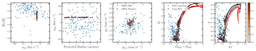
In Figure 1, we summarize the kinematics, chemistry, and stellar parameters of cluster members and MW foreground stars in our follow-up spectroscopic observations. The top panels from left to right compare the line-of-sight velocities ( $v_{los}$ ) to the stellar metallicity ([Fe/H]), the radial distance from the center of the cluster versus the $v_{los}$ , and the proper motion ( $\mu_{\alpha\star}$ , $\mu_{\delta}$ ). The member stars in each cluster are highlighted in different colours. Note in the proper motion panel, only stars with good quality astrometry are included. In the bottom panels we compare $v_{los}$ to the surface gravity (left, $\log{g}$ ), $v_{los}$ to effective temperature ( $T_{\rm eff}$ , center), and compare [Mg/Fe] vs [Fe/H]. Excluding LP 866, all stars are red giant branch/red clump stars (with several horizontal branch stars in Gran 3 and Gran 4). The derived properties of the star clusters are summarized in Table 2.

4.1 Cluster Properties and Spectroscopic Membership

We are able to identify the members of four clusters, Gran 3, Gran 4, Gaia 9, and Gaia 10, based purely on the line-of-sight velocity as the cluster mean velocity is distinct from the MW foreground. The stellar parameters ([Fe/H], $T_{\rm eff}$ , and $\log{g}$ ) and photometry ( $G$ , $G_{BP}$ , and $G_{RP}$ ) of the members identified from the velocities further reinforce their membership and they are consistent with single stellar populations. While there is a clear overdensity in the $v_{\rm los}$ distribution in the LP 866 and Garro 01 fields, there is overlap with the MW foreground and we construct mixture models to quantitatively identify members in these objects.

4.1.1 Gran 3/Patchick 125

In Figure 2, we summarize the Gran 3 members and the MW foreground stars from our M2FS observations of the Gran 3 field. In addition to the primary M2FS sample, we include 3 RRL members from the Gaia DR3 catalog (Clementini et al., 2022), 2 APOGEE members¹¹1First identified in Fernández-Trincado et al. (2022)., and 7 Gaia DR3 RVS members²²26 of the 7 of the members were first identified in Garro et al. (2023).. The 36 M2FS members of Gran 3 are identified by selecting stars in the $82<v_{\rm los}<97\mathrm{\,km}\mathrm{\,s}^{-1}$ velocity range. The M2FS stars all are consistent with a single metallicity and the stellar parameters ( $\log{\rm g}$ and $T_{\rm eff}$ ) are consistent with red giant stars or horizontal branch stars. There are two stars outside this range within $\sim 20~{}\mathrm{\,km}\mathrm{\,s}^{-1}$ of the mean velocity of Gran 3. The first, source_id³³3Here and throughout the paper source_id refers to Gaia DR3 source_id.=5977223144516980608, is a RRL star and the distance of this star agrees with the star cluster. We consider it a cluster member but we exclude this star from all kinematic analysis due to the velocity variability of RRL stars. The second, source_id=5977223144516066944, is a $7\sigma$ outlier in velocity but the stellar parameters agree with the cluster mean metallicity and the proper motion agrees with the cluster. We exclude it from our analysis and suggest that if it is a member, it is likely a binary star (e.g., Spencer et al., 2018). Additional multi-epoch data is required to confirm this.

To determine the kinematics and chemistry we use a two-parameter Gaussian likelihood function (Walker et al., 2006) and to use emcee to sample from the posterior (Foreman-Mackey et al., 2013). We use a uniform prior for the average and a Jeffreys prior for the dispersion. From the 35 stars in the M2FS sample that are non-variable, we measure $\overline{v_{\rm los}}=+90.9\pm 0.4~{}\mathrm{\,km}\mathrm{\,s}^{-1}$ , $\sigma_{v}=1.9\pm 0.3~{}\mathrm{\,km}\mathrm{\,s}^{-1}$ . With the 29 members with good quality [Fe/H] measurements, we measure $\overline{{\rm[Fe/H]}}=-1.83_{-0.04}^{+0.04}$ and $\sigma_{\rm[Fe/H]}=0.09\pm 0.4$ ( $\sigma_{\rm[Fe/H]}<0.16$ ). For limits throughout this work, we list values at 95% confidence intervals. We note that the non-zero metallicity dispersion is due to one star (source_id=5977224587625168768; $[{\rm Fe/H}]=-1.58\pm 0.07$ ) that is $3.5\sigma$ larger than the mean metallicity of Gran 3. This star has stellar parameters and mean velocity that are otherwise consistent with Gran 3. If this star is removed, the kinematics and mean metallicity are unchanged but the metallicity dispersion is constrained to less than $\sigma_{\rm[Fe/H]}<0.10$ . We have opted to include this star in our sample. From the 33 spectroscopically (M2FS, APOGEE, and Gaia RVS) identified members with good quality astrometry, we measure: $\overline{\mu_{\alpha\star}}=-3.74\pm 0.03\mathrm{\,\mathrm{\,mas}\mathrm{\,yr}^{-1}}$ , $\overline{\mu_{\delta}}=0.71_{-0.02}^{+0.01}\mathrm{\,\mathrm{\,mas}\mathrm{\,yr}^{-1}}$ , $\sigma_{\mu_{\alpha\star}}=0.10_{-0.02}^{+0.03}\mathrm{\,\mathrm{\,mas}\mathrm{\,yr}^{-1}}$ , $\sigma_{\mu_{\delta}}=0.03_{-0.01}^{+0.02}\mathrm{\,\mathrm{\,mas}\mathrm{\,yr}^{-1}}$ , and $\varpi=0.12\pm 0.01\mathrm{\,mas}$ . The parallax measurement corresponds to $d=8.6_{-0.8}^{+0.9}~{}\mathrm{\,kpc}$ and $(m-M)_{0}=14.7\pm 0.2$ , which is closer than the isochrone or RRL distance (see below). Assuming a distance of 10.5 kpc (in agreement with these latter measurements), the proper motion dispersions correspond to $\sigma_{\mu_{\alpha\star}}=5.0_{-1.1}^{+1.4}~{}\mathrm{\,km}\mathrm{\,s}^{-1}$ and $\sigma_{\mu_{\delta}}=1.7_{-0.7}^{+0.9}~{}\mathrm{\,km}\mathrm{\,s}^{-1}$ . While $\sigma_{\mu_{\alpha\star}}$ is larger than expected, $\sigma_{\mu_{\delta}}$ agrees with $\sigma_{v}$ . With the 7 Gaia RVS members we measure: $\overline{v_{\rm los}}=+93.5_{-1.5}^{+1.7}~{}\mathrm{\,km}\mathrm{\,s}^{-1}$ and $\sigma_{v}<6.6~{}\mathrm{\,km}\mathrm{\,s}^{-1}$ (95% c.i.). The Gaia RVS sample is consistent with the M2FS sample.

There are 3 stars in the secondary samples (1 APOGEE, 2 Gaia RVS) that are $\sim 9~{}\mathrm{\,km}\mathrm{\,s}^{-1}$ offset ( $1-5\sigma$ outliers in $v_{\rm los}$ ) from the bulk of Gran 3. 2 of these stars have repeat measurements with other samples and those measurements are in good agreement with the bulk velocity of the system and suggests that those stars could be binary stars. The APOGEE star (source_id=5977223316333009024; $v_{\rm los,~{}APOGEE}=100.2\pm 0.2\mathrm{\,km}\mathrm{\,s}^{-1}$ ) overlaps with Gaia RVS ( $v_{\rm los,~{}{\it Gaia}~{}RVS}=92.2\pm 2.2\mathrm{\,km}\mathrm{\,s}^{-1}$ ) and one of the Gaia RVS members source_id=5977224587625168768; ( $v_{\rm los,~{}{\it Gaia}~{}RVS}=99.2\pm 3.5\mathrm{\,km}\mathrm{\,s}^{-1}$ ) overlaps with M2FS ( $v_{\rm los,~{}M2FS}=92.6\pm 0.7\mathrm{\,km}\mathrm{\,s}^{-1}$ ). Both these stars may be binary stars which would explain their offset.

We identify three RRL in the Gaia DR3 RRL catalog (source_id=5977223144516980608, 5977224553266268928⁴⁴4We note that this star is a 3- $\sigma$ outlier in $\mu_{\delta}$ compared to the systemic proper motion, however, the large value of astrometric_excess_noise_sig suggests that the astrometric solution may not be reliable., 5977224557581335424) that are consistent with the proper motion and spatial position (all three have $R<2\arcmin$ ) of Gran 3. One star (source_id=5977223144516980608) was observed with M2FS. It is offset from the mean velocity of Gran 3 by $\sim 20\mathrm{\,km}\mathrm{\,s}^{-1}$ . As RRL stars are variable in velocity and vary more than $50\mathrm{\,km}\mathrm{\,s}^{-1}$ over the period (Layden, 1994), we consider this star a member. With more spectroscopic epochs the systemic velocity of the star could be measured (e.g., Vivas et al., 2005). We apply the metallicity correction to the absolute magnitude of a RRL in Gaia bands to determine the absolute magnitude: $M_{G}=0.32{\rm[Fe/H]}+1.11$ (Muraveva et al., 2018). From the three RRL, we find a mean distance modulus of $(m-M)_{0}=15.1$ corresponding to a distance of $d=10.5\mathrm{\,kpc}$ . This is slightly smaller than other distance measurements for this cluster: $d=12.02~{}\mathrm{\,kpc}$ (Gran et al., 2022), $d=11\pm 0.5~{}\mathrm{\,kpc}$ (Fernández-Trincado et al., 2022), and $d=10.9\pm 0.5,~{}11.2\pm 0.5~{}\mathrm{\,kpc}$ (Garro et al., 2022a).

In Figure 2, we compare an old (age $=13$ Gyr) and metal-poor isochrone ([Fe/H] = $-1.9$ ) to Gran 3 with both Gaia and DECaPS photometry. We are able to match the horizontal branch and the colour of the RGB if we use $(m-M)_{0}=15.2$ and a $R_{V}=3.3$ dust law (compared to a standard of $R_{V}=3.1$ ) and find it difficult to match the horizontal branch using the RRL distance. As noted by Garro et al. (2022a), some studies suggest a lower dust law is favored in the bulge regions (e.g., Souza et al., 2021; Saha et al., 2019) which would disagree with the RGB of Gran 3. This larger distance modulus is in better agreement with the literature distance measurements of Gran 3 (Gran et al., 2022; Fernández-Trincado et al., 2022; Garro et al., 2022a). We note that the brighter stars are bluer than the isochrone but the bulk of the RGB matches the isochrone.

4.1.2 Gran 4

The summary of our spectroscopic observations of Gran 4 is shown in Figure 3. We identify 64, 22, and 3 Gran 4 members in the M2FS, AAT and Gaia RVS sample, respectively, with the $-280<v_{\rm los}<-260\mathrm{\,km}\mathrm{\,s}^{-1}$ selection. 12 stars in the AAT sample overlap with the M2FS sample.

Within the M2FS sample, further examination of the velocity distribution reveals two outlier stars. The first (source_id=4077796986282497664) is a RRL star and is offset from the mean velocity by $\sim 8~{}\mathrm{\,km}\mathrm{\,s}^{-1}$ and by $\sim 3\sigma$ once the velocity dispersion is considered. It is a cluster member but due to its variable nature, we exclude it from any kinematic analysis. The second (source_id=4077796810168905344) is a $\sim 8\sigma$ outlier in velocity and if it is considered a member the velocity dispersion increases from $1.2~{}\mathrm{\,km}\mathrm{\,s}^{-1}$ to $2~{}\mathrm{\,km}\mathrm{\,s}^{-1}$ . It is consistent with the mean metallicity and proper motion of Gran 4, and the stellar parameters ( $T_{\rm eff}$ and $\log{g}$ ) are consistent with a red giant branch star. It seems unlikely for this star to be MW star based on the MW velocity and metallicity distribution, however, as it is a $\sim 8\sigma$ outlier it is either a binary star or a MW interloper and we exclude it from the analysis.

From the 62 non-variable M2FS members we find, $\overline{v_{\rm los}}=-266.4\pm 0.2~{}\mathrm{\,km}\mathrm{\,s}^{-1}$ , $\sigma_{v}=1.4\pm 0.2~{}\mathrm{\,km}\mathrm{\,s}^{-1}$ , $\overline{{\rm[Fe/H]}}=-1.84\pm 0.02$ and $\sigma_{\rm[Fe/H]}<0.10$ . Due to tail to zero dispersion and a lack of a clear peak, we do not consider the metallicity dispersion resolved and list an upper limit. The stellar parameters of these stars ( $T_{\rm eff}$ and $\log{g}$ ) are consistent with red giant branch stars or horizontal branch stars which further confirms our membership identification. With the 3 Gaia RVS members we measure: $\overline{v_{\rm los}}=-262.7_{-3.7}^{+3.6}~{}\mathrm{\,km}\mathrm{\,s}^{-1}$ , $\sigma_{v}<6.2~{}\mathrm{\,km}\mathrm{\,s}^{-1}$ (95% c.i.).

From the 22 AAT members, we find $\overline{v_{\rm los}}=-265.9\pm 0.4~{}\mathrm{\,km}\mathrm{\,s}^{-1}$ and $\sigma_{v}=1.5_{-0.3}^{+0.4}~{}\mathrm{\,km}\mathrm{\,s}^{-1}$ . 12 of these stars overlap with the M2FS sample. There is one velocity outlier (source_id=4077796397852026240) with $\sim 3\sigma$ , however, this star is in the M2FS sample with almost the exact same velocity. Removing this star decreases the velocity dispersion to $\sim 1~{}\mathrm{\,km}\mathrm{\,s}^{-1}$ from $\sim 1.5~{}\mathrm{\,km}\mathrm{\,s}^{-1}$ in the AAT sample but its inclusion or exclusion does not affect the M2FS kinematics and we opt to include it. From the calcium triplet metallicities, we compute $\overline{{\rm[Fe/H]}}=-1.82\pm 0.06$ and $\sigma_{\rm[Fe/H]}=0.21_{-0.05}^{+0.06}$ . The metallicity dispersion is clearly resolved in contrast to our expectation of a single stellar population in a star cluster and the lack of a metallicity dispersion in the M2FS sample. The source of the metallicity dispersion in the AAT data is unclear. As the M2FS sample is larger, we adopt the velocity and metallicity results from the M2FS sample as our primary results.

From the combined M2FS, AAT, and Gaia RVS sample there are 65 stars with good quality astrometric measurements. From these stars we measure: $\overline{\mu_{\alpha\star}}=+0.51\pm 0.01\mathrm{\,\mathrm{\,mas}\mathrm{\,yr}^{-1}}$ , and $\overline{\mu_{\delta}}=-3.51\pm 0.01\mathrm{\,\mathrm{\,mas}\mathrm{\,yr}^{-1}}$ , $\sigma_{\mu_{\alpha\star}}=0.02_{-0.01}^{+0.03}\mathrm{\,\mathrm{\,mas}\mathrm{\,yr}^{-1}}$ , $\sigma_{\mu_{\delta}}=0.05_{-0.03}^{+0.02}\mathrm{\,\mathrm{\,mas}\mathrm{\,yr}^{-1}}$ , and $\varpi=0.07\pm 0.01\mathrm{\,mas}$ . The parallax measurement corresponds to $d=14.6_{-1.9}^{+2.5}~{}\mathrm{\,kpc}$ and $(m-M)_{0}=15.8\pm 0.3$ which is closer than the other distance measurements (see below). Assuming a distance of 21.9 kpc (from the best-fit isochrone distance), the proper motion dispersion correspond to: $\sigma_{\mu_{\alpha\star}}=2.6_{-1.2}^{+2.7}\mathrm{\,km}\mathrm{\,s}^{-1}$ and $\sigma_{\mu_{\delta}}=5.4_{-2.8}^{+2.5}\mathrm{\,km}\mathrm{\,s}^{-1}$ .

We identify two RRL (source_id=4077796986282497664, 4077796573965756928) in the Gaia DR3 RRL catalog (Clementini et al., 2022) as members of Gran 4 based on their proper motion and distance. The first RRL is also in the VVV RRL (Molnar et al., 2022) and OGLE RRL catalogs (Soszyński et al., 2019). There is a third candidate RRL (source_id=4077796608325479168) from the PanSTARRS1 RRL catalog (Sesar et al., 2017), however, it is not in the Gaia DR3 RRL catalog so we do not include it in the analysis. It is considered a variable star in Gaia DR3 but only has a best_class_score=0.4 for being an RRL. Additional time series data are required to confirm the status of this star. From the two RRL members, $\mu=16.5,16.6$ corresponding to $d=19.9,21~{}\mathrm{\,kpc}$ . This is slightly closer than our best-fit $\mu\sim 16.7$ from matching the horizontal branch to a metal-poor isochrone. It is also closer than $\mu=16.84$ , $d=22.49~{}\mathrm{\,kpc}$ from Gran et al. (2022).

4.1.3 Garro 01

There is overlap in the MW foreground and star cluster velocity distributions for Garro 01 and LP 866 and we construct mixture models to account for this overlap. The total likelihood for our mixture models is:

\mathcal{L}=f_{\rm cluster}\mathcal{L}_{\rm cluster}+(1-f_{\rm cluster})\mathcal{L}_{\rm MW}\,,

(1)

where $\mathcal{L}_{\rm cluster}$ , $\mathcal{L}_{\rm MW}$ , and $f_{\rm cluster}$ correspond to the cluster population, the MW population, and the fraction of stars in the star cluster, respectively (e.g., Pace et al., 2020, 2021). We assume the probability distributions of each data component are separable:

\mathcal{L}_{\rm cluster/MW}=\mathcal{L}_{\rm spatial}\mathcal{L}_{\rm PM}\mathcal{L}_{\rm v_{los}}\mathcal{L}_{\rm[Fe/H]}\,.

(2)

Where $\mathcal{L}_{\rm spatial}$ , $\mathcal{L}_{\rm PM}$ , $\mathcal{L}_{\rm v_{los}}$ , and $\mathcal{L}_{\rm[Fe/H]}$ are the spatial likelihood, the proper motion likelihood, the line-of-sight velocity likelihood, and the metallicity likelihood, respectively. To compute the membership of each star, we compare the ratio of the cluster likelihood to total likelihood for each star: $p_{\rm member}=\mathcal{L}_{\rm cluster}/\mathcal{L}$ (e.g., Martinez et al., 2011).

For Garro 01, we primarily analyze a mixture model with $v_{\rm los}$ and [Fe/H] but also consider a second model with spatial information. We assume the $v_{\rm los}$ and [Fe/H] likelihood distributions are Gaussian for both the star cluster and MW components. We apply the following cuts to the Garro 01 spectroscopic sample to remove MW foreground stars: $T_{\rm eff}-2\times\sigma_{T_{\rm eff}}<6000K$ , $\log_{10}{g}-2\times\sigma_{\log_{10}{g}}<4$ , a parallax cut ( $\varpi-3\sigma_{\varpi}<0.064$ ), and a loose $G_{BP}-G_{RP}$ colour cut of 0.25 around an age = 11 Gyr and [Fe/H] = $-0.6$ MIST isochrone (Dotter, 2016). The isochrone selection is applied to remove blue MW main sequence stars from the sample which have no overlap in colour-magnitude space with the cluster members. From our primary mixture model, we find: $\overline{v_{\rm los}}=+31.0\pm 0.1~{}\mathrm{\,km}\mathrm{\,s}^{-1}$ , $\sigma_{v}=0.4\pm 0.3~{}\mathrm{\,km}\mathrm{\,s}^{-1}$ ( $\sigma_{v}<0.8~{}\mathrm{\,km}\mathrm{\,s}^{-1}$ ), $\overline{{\rm[Fe/H]}}=-0.30\pm 0.03$ and $\sigma_{\rm[Fe/H]}<0.14$ . In Figure 4, we summarize the properties of the spectroscopic members identified in the mixture model. Stars are coloured by their membership probability.

For the second spatial model we use a conditional likelihood and we assume that the fraction of stars is spatially dependent (e.g., Martinez et al., 2011; Pace et al., 2021):

f_{\rm cluster}(R)=\Sigma_{\rm cluster}(R)/(\Sigma_{\rm cluster}(R)+N\Sigma_{\rm MW}(R)).\\

(3)

Where $\Sigma$ is the projected stellar distribution and $N$ is the relative normalization between the cluster and MW spatial distributions We assume a King (1962) distribution for the Garro 01 distribution with parameters from Garro et al. (2020) and assume that the MW distribution is constant over the small region examined. We utilize a conditional likelihood as there is an unknown spatial selection function.

While the chemodynamic properties of Garro 01 from the two models are nearly identical, there are some minor differences in the membership of individual stars between the two models. The conditional likelihood model has larger membership for stars near the center and lower membership for the two most distant stars. The difference in membership between the models for individual stars is small ( $\sum|p_{\rm standard}-p_{\rm conditional}|=1.7$ ) and the overall membership is similar for the two models; both models have $\sum p=46.8\pm 1.9$ . We consider stars with $p>0.9$ as high confidence members and there are 39 and 42 members identified in the standard model and conditional likelihood model, respectively and note there are 43 high confidence members with $p>0.9$ in either model.

From the 42 members with good astrometry (42 M2FS and 1 Gaia RVS), we measure: $\overline{\mu_{\alpha\star}}=-4.35\pm 0.02~{}\mathrm{\,\mathrm{\,mas}\mathrm{\,yr}^{-1}}$ , $\overline{\mu_{\delta}}=-1.09\pm 0.02~{}\mathrm{\,\mathrm{\,mas}\mathrm{\,yr}^{-1}}$ , $\sigma_{\mu_{\alpha\star}}=0.09_{-0.02}^{+0.02}~{}\mathrm{\,\mathrm{\,mas}\mathrm{\,yr}^{-1}}$ , and $\sigma_{\mu_{\delta}}=0.08_{-0.02}^{+0.03}~{}\mathrm{\,\mathrm{\,mas}\mathrm{\,yr}^{-1}}$ . We measure $\varpi=0.08\pm 0.01\mathrm{\,mas}$ corresponding to $d=11.9_{-1.5}^{+2.1}~{}\mathrm{\,kpc}$ and $(m-M)_{0}=15.4\pm 0.3$ . The distance from the parallax is closer than the measurement derived from isochrone fits. Assuming a distance of 15.3 kpc from Garro et al. (2020), the proper motion dispersion terms correspond to: $\sigma_{\mu_{\alpha\star}}=6.6_{-1.4}^{+1.5}~{}\mathrm{\,km}\mathrm{\,s}^{-1}$ and $\sigma_{\mu_{\delta}}=5.8_{-1.8}^{+1.8}~{}\mathrm{\,km}\mathrm{\,s}^{-1}$ . Our proper motion measurement agrees with the Gaia DR2 proper motion measurement, $\overline{\mu_{\alpha\star}}=-4.68\pm 0.47~{}\mathrm{\,\mathrm{\,mas}\mathrm{\,yr}^{-1}}$ , and $\overline{\mu_{\delta}}=-1.35\pm 0.45~{}\mathrm{\,\mathrm{\,mas}\mathrm{\,yr}^{-1}}$ from Garro et al. (2020).

We identify 2 members in the Gaia RVS sample with velocities and proper motion consistent with Garro 01. Both stars are more evolved than the M2FS sample but roughly match the isochrone. Both stars are included in Figure 4 as purple circles.

We do not identify any RRL that have the same proper motion or a consistent distance with Garro 01. With the distance modulus of Garro et al. (2020), we can match the red clump of our spectroscopic sample with an isochrone and we adopt this distance for our analysis.

In Figure 4, we show optical colour-magnitude diagrams using Gaia and DECaPS photometry. The prominent feature in the CMDs is the red clump and complements the near-infrared discovery photometry from Garro et al. (2020). Our spectroscopic metallicity measurement is more metal-rich than the isochrone analysis of Garro et al. (2020) which found [Fe/H] = $-0.7$ with their CMDs fits (black isochrone in Figure 4). However, we cannot match the colour of the system with this age and spectroscopic metallicity. If we assume the spectroscopic metallicity, the isochrone is redder than the photometry. We discuss this in more detail in Section 5.1.

4.1.4 Gaia 9

We identify 19 M2FS members of Gaia 9 with the velocity selection: $150<v_{\rm los}<170~{}\mathrm{\,km}\mathrm{\,s}^{-1}$ . There is one star inside this velocity range (source_id=5537860050401680000) that is a non-member based on its proper motion. The properties of the members and proper motion selected stars are displayed in Figure 5. From the 19 members, we measure: $\overline{v_{\rm los}}=+159.0\pm 0.3~{}\mathrm{\,km}\mathrm{\,s}^{-1}$ , $\sigma_{v}=1.0\pm 0.3~{}\mathrm{\,km}\mathrm{\,s}^{-1}$ , $\overline{{\rm[Fe/H]}}=-0.50\pm 0.06$ and $\sigma_{\rm[Fe/H]}<0.16$ . There is one additional member Gaia RVS that we identify (source_id=5537859848550503168) based on the radial velocity and proper motion and we include it in Figure 5. From the 19 members with good astrometry, we measure: $\overline{\mu_{\alpha\star}}=-1.08\pm 0.03~{}\mathrm{\,\mathrm{\,mas}\mathrm{\,yr}^{-1}}$ , $\overline{\mu_{\delta}}=+1.50\pm 0.03~{}\mathrm{\,\mathrm{\,mas}\mathrm{\,yr}^{-1}}$ , $\sigma_{\mu_{\alpha\star}}=0.07\pm 0.04~{}\mathrm{\,\mathrm{\,mas}\mathrm{\,yr}^{-1}}$ , $\sigma_{\mu_{\delta}}=0.08_{-0.03}^{+0.03}~{}\mathrm{\,\mathrm{\,mas}\mathrm{\,yr}^{-1}}$ , and $\varpi=0.08\pm 0.01\mathrm{\,mas}$ . The parallax measurement corresponds to $d=12.9_{-2.0}^{+3.0}~{}\mathrm{\,kpc}$ and $(m-M)_{0}=15.6_{-0.4}^{+0.5}$ which agrees with our isochrone derived distance (see below). Assuming a distance of 13.8 kpc (from our isochrone derived distance), the proper motion dispersion terms correspond to: $\sigma_{\mu_{\alpha\star}}=4.8_{-2.4}^{+2.4}~{}\mathrm{\,km}\mathrm{\,s}^{-1}$ and $\sigma_{\mu_{\delta}}=5.0_{-2.1}^{+2.3}~{}\mathrm{\,km}\mathrm{\,s}^{-1}$ .

In the Gaia colour-magnitude diagram (Figure 5), the majority of the spectroscopic members are red clump stars. We estimate the distance of the cluster to be $(m-M)_{0}=15.7$ or $d=13.8~{}\mathrm{\,kpc}$ based on the red clump using an MIST isochrone with age = 1.5 Gyr and [Fe/H] = $-0.5$ . The blue stars at $G_{0}\sim 17$ are likely the top of the main sequence and we use this feature to assist in estimating the age of the system. Gaia 9 is younger than the other clusters examined thus far and it likely an open cluster.

4.1.5 Gaia 10

Gaia 10 has similar properties to Gaia 9 but is more distant. We summarize our spectroscopic sample in Figure 6. We identify 23 members of Gaia 10 with a velocity selection: $v_{\rm los}>120\mathrm{\,km}\mathrm{\,s}^{-1}$ . Two stars (source_id=5534905976200827776 and 5540909996882971520) have kinematics (line-of-sight velocity and proper motion) that agree with the cluster but both stars are significant outerliers in metallicity. 5534905976200827776 is $3.2\sigma$ more metal-rich while 5540909996882971520 is $4.9\sigma$ more metal-poor and the inclusion of either star results in an offset mean metallicity and non-zero metallicity dispersion. We consider both stars non-members. The inclusion of the star as a members would infer to a non-zero metallicity dispersion. We note that this same star is in the Gaia RVS catalog with a similar velocity. From the spectroscopic members, we measure: $\overline{v_{\rm los}}=+135.9\pm 0.4~{}\mathrm{\,km}\mathrm{\,s}^{-1}$ , $\sigma_{v}=1.4_{-0.3}^{+0.4}~{}\mathrm{\,km}\mathrm{\,s}^{-1}$ , $\overline{{\rm[Fe/H]}}=-0.34\pm 0.06$ and $\sigma_{\rm[Fe/H]}<0.14$ .

From the 21 members with good astrometry, we measure: $\overline{\mu_{\alpha\star}}=-0.74\pm 0.03~{}\mathrm{\,\mathrm{\,mas}\mathrm{\,yr}^{-1}}$ , $\overline{\mu_{\delta}}=+1.60_{-0.03}^{+0.04}~{}\mathrm{\,\mathrm{\,mas}\mathrm{\,yr}^{-1}}$ , $\sigma_{\mu_{\alpha\star}}=0.05_{-0.03}^{+0.05}~{}\mathrm{\,\mathrm{\,mas}\mathrm{\,yr}^{-1}}$ , $\sigma_{\mu_{\delta}}=0.06_{-0.03}^{+0.04}~{}\mathrm{\,\mathrm{\,mas}\mathrm{\,yr}^{-1}}$ , and $\varpi=0.09\pm 0.02\mathrm{\,mas}$ . The parallax measurement corresponds to $d=10.8_{-1.9}^{+3.1}~{}\mathrm{\,kpc}$ and $(m-M)_{0}=15.2_{-0.4}^{+0.6}$ which is much closer than our isochrone derived distance (see below). Assuming a distance of 17.4 kpc (from our isochrone derived distance), the proper motion dispersion terms correspond to: $\sigma_{\mu_{\alpha\star}}=4.2_{-2.6}^{+3.8}~{}\mathrm{\,km}\mathrm{\,s}^{-1}$ and $\sigma_{\mu_{\delta}}=5.0_{-2.8}^{+3.5}~{}\mathrm{\,km}\mathrm{\,s}^{-1}$ .

We compare theoretical isochrones based on the spectroscopic metallicity to the Gaia colour-magnitude diagram Figure 6. With an age of $1~{}{\rm Gyr}$ and distance modulus of $(m-M)_{0}=16.2$ ( $d=17.4~{}\mathrm{\,kpc}$ ) we can fit the red clump and the possible main sequence turnoff based on the proper motion selected sample. Similar to Gran 3, to match the colour of the isochrone a larger extinction coefficient of $R_{V}=3.3$ is required. There remains considerable spread in the colour of the members. This may be due to differential reddening. We consider Gaia 10 an open cluster.

4.1.6 LP 866

LP 866 is the only star cluster where the entirety of the M2FS spectroscopic sample is located on the main-sequence. Similar to Garro 01, we run a mixture model to account for the MW foreground distribution with $v_{\rm los}$ , proper motion, and [Fe/H] components. We do not include a conditional likelihood run as the spatial distribution was not known beforehand. We assume the proper motion distribution is a truncated multi-variate Gaussian for both components with limits: $1.5<\mu_{\alpha\star}<3.5~{}{\rm mas~{}yr^{-1}}$ , $-0.4<\mu_{\delta}<1.2~{}{\rm mas~{}yr^{-1}}$ . While the proper motion was included in the spectroscopic target selection (based on Gaia DR2 astrometry), the proper motion dispersion is resolved in contrast to the other star clusters. We excluded stars outside of this proper motion limit and two bright stars with discrepant parallax measurements.

With the mixture model, we identify 80 high confidence members ( $p>0.9$ ) and measure the following properties for LP 866: $\overline{v_{\rm los}}=-9.8\pm 0.1~{}\mathrm{\,km}\mathrm{\,s}^{-1}$ , $\sigma_{v}=0.6\pm 0.1~{}\mathrm{\,km}\mathrm{\,s}^{-1}$ , $\overline{{\rm[Fe/H]}}=0.10\pm 0.03$ , $\sigma_{\rm[Fe/H]}=0.15\pm 0.04$ ( $\sigma_{\rm[Fe/H]}<0.22$ ), $\overline{\mu_{\alpha\star}}=2.93_{-0.02}^{+0.01}~{}\mathrm{\,\mathrm{\,mas}\mathrm{\,yr}^{-1}}$ , $\overline{\mu_{\delta}}=0.44_{\pm}0.02~{}\mathrm{\,\mathrm{\,mas}\mathrm{\,yr}^{-1}}$ , $\sigma_{\mu_{\alpha\star}}=0.08_{-0.02}^{+0.02}~{}\mathrm{\,\mathrm{\,mas}\mathrm{\,yr}^{-1}}$ , and $\sigma_{\mu_{\delta}}=0.10_{-0.01}^{+0.02}~{}\mathrm{\,\mathrm{\,mas}\mathrm{\,yr}^{-1}}$ . The overall membership is $\sum p=86.4\pm 4.8$ . As there is a non-zero metallicity dispersion, it is possible that our model has incorrectly identified some MW stars as cluster members. From the 86 members with good astrometry, we measure $\varpi=0.437\pm 0.005\mathrm{\,mas}$ corresponding to $d=2.29\pm 0.03~{}\mathrm{\,kpc}$ and $(m-M)_{0}=11.80\pm 0.02$ . Assuming a distance of 2.29 kpc, the proper motion dispersion terms correspond to: $\sigma_{\mu_{\alpha\star}}=0.9\pm 0.02~{}\mathrm{\,km}\mathrm{\,s}^{-1}$ and $\sigma_{\mu_{\delta}}=1.1\pm 0.2~{}\mathrm{\,km}\mathrm{\,s}^{-1}$ .

In the Gaia RVS sample there is a clear overdensity and velocity peak distinct from the MW population within the central 8′of LP 866. We find 14 stars in the Gaia RVS catalog that are consistent with the velocity, proper motion, and parallax of LP 866. All 14 stars are more evolved than the M2FS sample and aid in matching a stellar isochrone. With the 14 Gaia RVS members we find: $\overline{v_{\rm los}}=-10.6\pm 0.8~{}\mathrm{\,km}\mathrm{\,s}^{-1}$ , and $\sigma_{v}=0.2_{-0.1}^{+0.9}~{}\mathrm{\,km}\mathrm{\,s}^{-1}$ ( $\sigma_{v}<2.2~{}\mathrm{\,km}\mathrm{\,s}^{-1}$ ); and from the 12 stars with good quality astrometry we find: $\overline{\mu_{\alpha\star}}=2.88\pm 0.01~{}\mathrm{\,\mathrm{\,mas}\mathrm{\,yr}^{-1}}$ , and $\overline{\mu_{\delta}}=0.44\pm 0.02~{}\mathrm{\,\mathrm{\,mas}\mathrm{\,yr}^{-1}}$ . These results are consistent with the M2FS sample.

We include Gaia and DECaPs colour magnitude diagrams in Figure 7. We match theoretical isochrones to estimate the age of the system. Unlike the other two open clusters, we have a confident distance and metallicity measurement. We find that reducing the E(B-V) by $\sim 53\%$ and setting the to age = $10^{9.5}$ = $\sim$ 3 Gyr provides an adequate match. We note that the we varied the extinction to match the RGB of the Gaia RVS stars and varied the age to match the main sequence turn-off of the M2FS sample with the Gaia photometry. The same isochrone provided an similarly adequate match to the g-r vs g DECaPs photometry. More in depth modeling is required to improve constraints on the age and extinction of the cluster. Regardless, we consider LP 866 an open cluster.

4.2 Spatial Distribution

To measure the spatial distribution of each star cluster, we construct a larger proper motion selected sample from the Gaia DR3 catalog based on the systemic proper motion found from our spectroscopic sample and apply a spatial mixture model (Equations 1, 2). We do not apply this methodology to the spectroscopic sample as it is not spatially complete and has an unknown spatial target selection. For the spatial likelihood we model the star cluster with two density profiles. The first profile is a Plummer distribution (Plummer, 1911):

\Sigma(R)=\frac{1}{\pi r_{p}^{2}}\frac{1}{\left(1+\left(R/r_{p}\right)^{2}\right)^{2}}

(4)

where $r_{p}$ is the Plummer scale radius (for a Plummer profile $r_{p}$ is equivalent to the 2D deprojected half-light radius). The second is the King profile (King, 1962):

\Sigma_{\star}(R)\propto\left[\left(1+\frac{R^{2}}{r_{c}^{2}}\right)^{-1/2}-\left(1+\frac{r_{t}^{2}}{r_{c}^{2}}\right)^{-1/2}\>\right]^{2}

(5)

where $r_{c}$ is the core radius and $r_{t}$ is the tidal radius. We model a small region near each cluster and assume that the MW background is constant within that small area after a proper motion selection is applied.

For the Gaia selected sample, we apply the following cuts: a 3- $\sigma$ selection in proper motion, a parallax selection ( $\varpi-\varpi_{\rm cluster}-3\sigma_{\varpi}<0$ ), $G<20$ , $R<R_{\rm max}$ , and stars with good astrometry (i.e., satisfy our astrometric cuts in Section 3.4). We will refer to this Gaia selected sample and utilize the same sample for examining the colour-magnitude diagrams of the clusters. We use $R_{\rm max}=12\arcmin$ for LP 866 and $R_{\rm max}=6\arcmin$ for all other clusters. For Garro 01 we additionally apply a loose $G_{BP}-G_{RP}$ colour cut of 0.25 around an age = 11 Gyr and [Fe/H] = $-0.6$ MIST isochrone (Dotter, 2016) following the spectroscopic selection. For the other clusters, the above selection primarily identifies stars with a stellar population that agrees with the spectroscopic sample. Any photometric outliers (i.e., MW stars) will be roughly distributed uniformly within the small area examined and not bias the spatial distribution calculations.

The Plummer and King fits along with the binned stellar profile of all six clusters are shown in Figure 8. In general, the results from the Plummer and King profile fits agree and provide adequate fits. Due to the low number of stars, there is no preference for one profile over the other. We are unable to constrain $r_{t}$ and generally only provide lower limits. For the globular clusters, we find $r_{h}=1.7\pm 0.2\arcmin$ , $r_{h}=2.2_{-0.4}^{+0.5}\arcmin$ , and $r_{h}=2.4_{-0.4}^{+0.6}~{}\arcmin$ corresponding to $r_{h}=5.3_{-0.6}^{+0.7}~{}\mathrm{\,pc}$ , $r_{h}=14.2_{-2.5}^{+3.3}~{}\mathrm{\,pc}$ , and $r_{h}=10.9_{-2.0}^{+2.6}~{}\mathrm{\,pc}$ from the Plummer profile fits for Gran 3, Gran 4, and Garro 01, respectively. With the King profile, we find $r_{c}=1.1_{-0.2}^{+0.3}\arcmin$ , $r_{c}=1.4_{-0.4}^{+0.5}\arcmin$ , and $r_{c}=1.8_{-0.5}^{+0.7}~{}\arcmin$ for Gran 3, Gran 4, and Garro 01, respectively. For comparison, Gran et al. (2022) find $r_{h}=1.05\pm 0.04\arcmin$ and $r_{h}=1.14\pm 0.02\arcmin$ , for Gran 3 and Gran 4, respectively. These are smaller than the sizes we infer. Garro et al. (2020) measure $r_{c}=2.5\pm 1.5\arcmin$ for Garro 01 and a poorly constrained $r_{t}$ which agrees with our measurement.

For the open clusters, we find $r_{h}=1.4\pm 0.2\arcmin$ , $r_{h}=1.6_{-0.2}^{+0.3}\arcmin$ , and $r_{h}=4.6_{-0.6}^{+0.7}\arcmin$ with the Plummer profile fits for Gaia 9, Gaia 10, and LP 866, respectively. With the King profile, we find $r_{c}=0.8\pm 0.2\arcmin$ , $r_{c}=1.0_{-0.2}^{+0.3}\arcmin$ , and $r_{c}=3.3_{-0.7}^{+0.8}~{}\arcmin$ for Gaia 9, Gaia 10, and LP 866, respectively. The results for the six clusters are included in Table 2.

4.3 Orbital Properties

We use the gala package to compute the orbits of the six star clusters and compare them to other MW globular clusters. We use the default MilkyWayPotential Galactic potential from Price-Whelan (2017). This potential consists of two Hernquist (1990) spheroids to model the stellar bulge and nucleus, a Miyamoto & Nagai (1975) axisymmetric stellar disk, and a NFW dark matter halo (Navarro et al., 1996). For each cluster we compute the integrals of motion, $E$ and $L_{z}$ , the approximately conserved quantity $L_{\perp}$ (Massari et al., 2019) and the orbital pericenter ( $r_{\rm peri}$ ), apocenter ( $r_{\rm apo}$ ), and eccentricity. We list the results in Table 2. We apply the same analysis to the MW globular clusters using the phase space results from Vasiliev & Baumgardt (2021). We compute 1000 orbits drawn from each satellite’s 6D phase distribution in Table 2 and compute statistics from these runs. We use the astropy v4.0 frame (Astropy Collaboration et al., 2013, 2018) for the Sun’s position and velocity: distance to Galactic Center, $D_{\odot}=8.122\mathrm{\,kpc}$ , $v_{\odot}=(12.9,245.6,7.78)~{}\mathrm{\,km}\mathrm{\,s}^{-1}$ (Drimmel & Poggio, 2018; Gravity Collaboration et al., 2018; Reid & Brunthaler, 2004).

In Figures 9 and 10, we show 5 example orbits drawn from the observational errors of each cluster. Gran 3 is on a near circular orbit ( $e\sim 0.12$ ) in the inner bulge ( $R_{GC}\sim 2.7\mathrm{\,kpc}$ ) that is confined to the plane of the disk ( $z_{max}\sim 1.8\mathrm{\,kpc}$ ). Gran 3 is on a retrograde orbit ( $L_{Z}\sim+0.45~{}{\rm kpc^{2}~{}Myr^{-2}}$ ). Gran 4 has an eccentric orbit ( $e\sim 0.63$ ) with a small pericenter ( $r_{\rm peri}\sim 8~{}\mathrm{\,kpc}$ ), large apocenter ( $r_{\rm apo}\sim 35~{}\mathrm{\,kpc}$ ), and is not confined to the MW midplane ( $z_{\rm max}\sim 21~{}\mathrm{\,kpc}$ ). Gran 4 is an halo globular cluster that is currently near passing the MW midplane. We find that Garro 01 is on a circular orbit ( $e\sim 0.16$ ) that is confined to the Galactic midplane ( $z_{\rm max}\sim 1.3~{}\mathrm{\,kpc}$ ) at a relatively large Galactocentric radius ( $\sim 10-13~{}\mathrm{\,kpc}$ ). The orbits of the three younger open clusters are all circular ( ${\rm ecc}\sim 0.1-0.16$ ), disk-like orbits. Relative to other open clusters Gaia 9 and Gaia 10 are at large Galactic distances ( $R_{\rm GC}\sim 18~{}{\rm and}\sim 21~{}\mathrm{\,kpc}$ ) and have higher angular momentum $L_{Z}\sim-3.5--4.7~{}{\rm kpc^{2}~{}Myr^{-2}}$ . The largest source of uncertainty in our orbit modeling comes from the distance measurement.

5 Discussion

We have presented accurate kinematics and metallicity measurements from Magellan/M2FS spectroscopy for three recently discovered globular clusters, Gran 3, Gran 4 and Garro 01, and the discovery and spectroscopic confirmation of three young open clusters, Gaia 9, Gaia 10, and LP 866. Here we consider our results in the context of the MW star cluster population.First, we comment on the nature of Garro 01 and whether it is an old globular cluster or open cluster (Section 5.1). In particular, how do Gran 3, Gran 4 and Garro 01 relate to the MW globular cluster population and other recently discovered clusters (Section 5.3)? Are these new globular clusters connected to accretion events or were they formed in-situ (Section 5.4)? How do the open clusters compare to the Galactic radial metallicity gradient (Section 5.5)? We conclude by comparing our results to the literature.

5.1 The Nature of Garro 01

Garro et al. (2020) classify Garro 01 as a globular cluster based on its close similarity to the globular cluster 47 Tuc but several magnitudes fainter. Our spectroscopic metallicity is more metal-rich ([Fe/H] $=-0.3$ ) than the photometric analysis ([Fe/H] $=-0.7$ ). The orbit of Garro 01 is a disk-like orbit and Garro 01 is confined to the Galactic plane ( $z_{\rm max}\sim 1.3~{}\mathrm{\,kpc}$ , ${\rm ecc}\sim 0.16$ ). Both properties are consistent with the open cluster population. The age of a star cluster can be key for determining its origin as a globular cluster or open cluster (e.g., Garro et al., 2022a).

As previously noted, we had difficultly matching the spectroscopic metallicity and literature age ( $11\pm 1$ Gyr) with Gaia and DECaPS photometry as the isochrone was redder than the photometry. To estimate the age, we vary the age at a fixed metallicity ([Fe/H] $=-0.3$ ) and check whether the color of the red-giant branch is matched. For this exercise, we examine both Gaia, $G_{BP}-G{RP}$ , and DECaPS, $g-r$ , and $r-i$ color. Our best estimate for the age between $2-13$ Gyr is 4 Gyr (red isochrone in Figure 4). For younger ages $<3.5~{}{\rm Gyr}$ , the main sequence turn-off would be apparent in our sample which we do not observe. The isochrones with older ages ( $>6$ Gyr) are redder than the observed data. In addition, we find that the Gaia RVS candidate members are better fit with the younger age.

An age of $\sim 4~{}{\rm Gyr}$ suggests that Garro 01 is an open cluster. This agrees with the metallicity and disk-like orbit of Garro 01. An accurate age measurement from deeper photometry would confidently classify this star cluster as either an open or globular cluster. For the reminder of the discussion, we will analyze Garro 01 with both the globular clusters and open clusters in our sample.

5.2 Globular Cluster Kinematics

Globular clusters have more complex kinematics than the simple constant velocity dispersion model we have explored including rotation (e.g., Sollima et al., 2019) and velocity dispersion profiles (Baumgardt & Hilker, 2018). We search for rotation by comparing the difference between the mean line-of-sight velocity across different position angles. We show the results of this exercise in Figure 11. There is potential rotation on the order of $\sim 1-2\mathrm{\,km}\mathrm{\,s}^{-1}$ in the three clusters, however, when considering the mean velocity errors it is not significant.

In general, globular clusters have velocity dispersion profiles that decrease with radius (e.g., Baumgardt & Hilker, 2018) and we search for a radial dependence in the velocity dispersion by binning the data. We show the binned velocity dispersion profiles of the three globular clusters in Figure 12. Each bin contains 18 (Gran 3), 16 (Gran 4), and 15 stars (Garro 01). For Gran 4 we show the results with the M2FS data (blue) and combined M2FS + AAT data⁵⁵5There is a $-1.36\mathrm{\,km}\mathrm{\,s}^{-1}$ offset applied to the AAT data based on the repeat measurements. (orange). Combining the AAT and M2FS data only increases the sample by 12 stars but there are 10 stars with improved velocity precision due to multiple measurements. The M2FS velocity dispersion profiles of Gran 3 and Gran 4 clearly decrease with radius. The combined M2FS + AAT profile of Gran 4 is more consistent with the constant dispersion model but the central bin has a larger velocity dispersion. With Garro 01 the binned profile only measures an upper limit, similar to the global fit in our mixture model.

To better constrain and quantify the velocity dispersion profile and/or rotation we explore detailed models. We model the velocity dispersion with a Plummer profile (Plummer, 1911) and the radially dependent velocity dispersion profile is: $\sigma^{2}(R)=\sigma_{0}^{2}/\sqrt{1+(r/r_{0})^{2}}$ , where $\sigma_{0}$ , and $r_{0}$ are free parameters. We use the following rotation profile (e.g., Mackey et al., 2013; Cordero et al., 2017; Alfaro-Cuello et al., 2020): $V_{\rm rot}=\frac{2V_{\rm max}}{r_{\rm peak}}\frac{X_{PA}}{1+\left(X_{PA}/r_{\rm peak}\right)^{2}}$ , where $V_{\rm max}$ , $r_{\rm peak}$ , and $\theta_{PA}$ (which determines $X_{PA}$ ) are free parameters. We use the dynesty package to sample the posterior and compute Bayesian evidence for model comparison (Speagle, 2020; Koposov et al., 2022).

We apply the velocity dispersion and rotation models both separately and together for all three clusters. The inferred velocity dispersion profile fits are included in Figure 12 with their corresponding errors. For Garro 01 we examine the stars with membership $>0.9$ . For all three clusters the functional velocity dispersion profile is favored over the constant, non-rotating model but it is not favored at a statistically significant level. The dispersion models for Gran 3 and Gran 4 both favor a larger dispersion in the center of the clusters that decreases with radius. In terms of Bayesian evidence⁶⁶6We use the scale of Trotta (2008) to quantify significance. $\ln{Z}$ ranges of 0-1, 1-2.5, 2.5-5.5, $>5.5$ correspond to inconclusive, weak, moderate, and substantial evidence in favor of the new model., we find $\ln{Z}=1.7,~{}0.7,~{}0.3$ in favor of the $\sigma(R)$ model for Gran 3, Gran 4, and Garro 01, respectively. Gran 3 is favored with weak evidence whereas the others are inconclusive. No rotation models are favored and the rotation models produce an upper limit to the rotation. The rotation models do have a non-zero peak but large portions of the posterior remain consistent with no rotation. While there are coherent rotation signals in Figure 11, the non-zero velocity dispersion and errors in the rotation curve are consistent with no rotation. To improve constraints on the velocity dispersion profile or probe potential rotation, larger samples of stars are required.

Last, we estimate the dynamical mass and corresponding mass-to-light ratio of the three globular clusters. Specifically, we compute the dynamical mass using the dispersion supported mass estimator from Errani et al. (2018): $M(r<1.8R_{h})\approx 3.5\times 1.8R_{h}\langle\sigma^{2}_{\rm los}\rangle G^{-1}$ . This approximator is insensitive to the unknown underlying velocity anisotropy (Walker et al., 2009; Wolf et al., 2010; Errani et al., 2018) but assumes that the velocity dispersion is approximately constant with radius which may not be true for globular clusters or the globular clusters in our sample. With our line-of-sight velocity dispersion and half-light radii measurements, we measure $M(r<1.8R_{h})=2.7\times 10^{4}\mathrm{\,M_{\odot}}$ , $4.0\times 10^{4}\mathrm{\,M_{\odot}}$ , and $2.3\times 10^{3}\mathrm{\,M_{\odot}}$ ( $<1.1\times 10^{4}\mathrm{\,M_{\odot}}$ ) for Gran 3, Gran 4, and Garro 01, respectively. The corresponding mass-to-light ratios are⁷⁷7For reference, a Plummer profile at $r=1.8r_{\rm p}$ encloses 66.8% of the total mass. are 1.8 and $0.2$ ( $<1.1$ ), for Gran 4 and Garro 01, respectively. There are two literature $M_{V}$ values for Gran 3: $M_{V}=-3.8$ (Garro et al., 2022a) and $M_{V}=-6.02$ (Gran et al., 2022). These correspond to mass-to-light ratios of 1.8 (for $M_{V}=-6.02$ ) and 14.2 (for $M_{V}=-3.8$ ). The mass-to-light ratios for Gran 3 and Gran 4 agree with old stellar populations. More detailed dynamical modeling, focused on star clusters would improve this analysis (e.g., Gieles & Zocchi, 2015; Song et al., 2021).

5.3 Comparison to the Globular Cluster Population

In Figure 13, we compare the sizes (based on the 2D projected half-light radii, $R_{h}$ ), the metallicity ([Fe/H]), and absolute magnitudes ( $M_{V}$ ) of our globular cluster sample (Gran 3, Gran 4, Garro 01) to the MW globular cluster population (Harris, 1996) and to other recently discovered globular clusters (or candidates) at low Galactic latitude. The (incomplete) list of recently discovered globular clusters primarily in the Galactic disk and bulge includes: FSR 1758 (Barbá et al., 2019; Vasiliev & Baumgardt, 2021; Myeong et al., 2019; Romero-Colmenares et al., 2021), FSR 19 (Obasi et al., 2021), FSR 25 (Obasi et al., 2021), Garro 2 (Garro et al., 2022b), ESO456-29/Gran 1 (Gran et al., 2019), Gran 2, Gran 5 (Gran et al., 2022), Patchick 99 (Garro et al., 2021), Pfleiderer 2 (Ortolani et al., 2009), Ryu 059, Ryu 879 (Ryu & Lee, 2018), VVV CL001 (Minniti et al., 2011; Olivares Carvajal et al., 2022), VVV CL002 (Moni Bidin et al., 2011), VVV CL160 (Minniti et al., 2021), Sagittarius II (Mutlu-Pakdil et al., 2018; Longeard et al., 2021), and Crater 1 (Weisz et al., 2016; Kirby et al., 2015). We note that the classification of some objects is uncertain and spectroscopy is needed.

Our globular cluster sample is generally fainter than the MW globular cluster population which explains their recent discovery with Gaia astrometry. Gran 4 and Garro 01 are both larger than most clusters ( $r_{h}>10~{}\mathrm{\,pc}$ ). The large size of Garro 01 is particularly unusual as almost all metal-rich ([Fe/H] $>-1.5$ ) MW globular clusters have smaller sizes ( $r_{h}<10~{}\mathrm{\,pc}$ ). The exceptions to this are Palomar 12, which is associated with Sagittarius (e.g., Law & Majewski, 2010; Massari et al., 2019), and the Fornax 6 globular cluster associated with the Fornax dwarf spheroidal galaxy (Wang et al., 2019; Pace et al., 2021). Unlike the other large clusters, Garro 01 is on a circular disk-like orbit making it less likely to have an ex-situ origin. Gran 3 and Gran 4 are in the metal-poor tail of the MW globular cluster population as they are more metal-poor than $\sim 83\%$ of the globular clusters in the Harris catalog. In contrast, Garro 01 is one of the more metal-rich globular clusters. If Garro 01 is confirmed as a younger open cluster that could explain its large size compared to other metal-rich globular clusters. In summary, Gran 3, Gran 4, and Garro 01 have properties consistent with the MW globular cluster population.

5.4 Origin and Connection to Accretion Events

The MW has a population of in-situ and accreted/ex-situ globular clusters (e.g., Myeong et al., 2018; Massari et al., 2019; Kruijssen et al., 2019). To determine whether Gran 3, Gran 4, and Garro 01 are associated with any accretion events we compare the orbital properties of our sample to globular clusters associated with known events. In Figure 14, we compare the orbital properties of our globular cluster sample with the MW globular cluster population. Specifically we examine the energy, angular momentum in the z-direction, and the angular momentum in the perpendicular direction, and the pericenter and apocenter. We group the MW clusters based on accretion/merger events⁸⁸8We have not included the Sequoia+Arjuna+Iiloi structures (Myeong et al., 2019; Naidu et al., 2020), or Pontus structure (Malhan, 2022) mergers as there is little overlap with the three globular clusters in our sample. Furthermore, Thamnos is not included as there are no known globular clusters. , including: Sagittarius (Sgr), Gaia-Sausage/Enceladus (GSE) (Belokurov et al., 2018; Helmi et al., 2018), LMS-1/Wukong (Yuan et al., 2020; Naidu et al., 2020), Aleph (Naidu et al., 2020), Cetus (Newberg et al., 2009), the Helmi stream (Helmi et al., 1999; Koppelman et al., 2019a), low-energy/Koala/Kraken/Heracles (Massari et al., 2019; Kruijssen et al., 2019, 2020; Forbes, 2020; Horta et al., 2021) and the in-situ bulge population. We use Malhan et al. (2022) to associate globular clusters and merger events for GSE (we additionally include globular clusters from Massari et al. 2019 for the GSE sample), Sgr, Cetus, LMS-1/Wukong, and the in-situ bulge population. We follow Naidu et al. (2020) to associate Palomar 1 and the Aleph structure. The association of the Helmi stream globular clusters is taken from Callingham et al. (2022). We note between different analyses there is overlap between the globular clusters assigned to the Helmi stream, GSE, and LMS-1/Wukong accretion events. The Malhan (2022) analysis does not associate any globular clusters with the Helmi streams and the Callingham et al. (2022) analysis does not associate any globular clusters with the LMS-1/Wukong merger. For the Kraken merger, we use the identification from Callingham et al. (2022). The Kraken globular clusters overlap with the low-energy globular clusters from Massari et al. (2019), the Heracles accretion event (Horta et al., 2021) and the Koala merger from Forbes (2020) and all may be the same merger event. For simplicity we only include the Kraken merger. We note the Kraken/Koala/Heracles mergers (and associated globular clusters) in terms of their chemistry are consistent with being born in-situ, in a pre-disk population known as Aurora (Belokurov & Kravtsov, 2022). The identification of each globular cluster with a particular merger event depends on the methodology and sample (e.g., globular cluster, stellar stream, halo star), and different analyses have assigned the same globular cluster to different events or the in-situ population.

In the $E$ - $L_{Z}$ plane Gran 3 is located near globular clusters associated with the Galactic bulge and the low-energy/Koala/Kraken merger (Massari et al., 2019; Kruijssen et al., 2019, 2020; Forbes, 2020). Gran 3 may be an extension the Galactic bulge component to higher energy. The Kraken globular clusters generally have smaller $L_{Z}$ than Gran 3 and have prograde orbits with larger eccentricity (Massari et al., 2019; Kruijssen et al., 2019, 2020; Forbes, 2020). As this was one of the first MW mergers the globular clusters have low metallicities, similar to Gran 3. While there is overlap, the retrograde orbit of Gran 3 disfavors an association with the Kraken merger. There are several retrograde accretion events in the stellar halo including the Sequoia+Arjuna+Iiloi event (Malhan et al., 2022) and Thamnos structure (Koppelman et al., 2019b). The Thamnos structure has the lowest energy of the retrograde structures and has a similar metallicity to Gran 3 (Naidu et al., 2020; Horta et al., 2023), however, the energy is larger than Gran 3 and it is unlikely for Gran 3 to be associated with the Thamnos merger. We consider Gran 3 to be a member of the Galactic bulge globular cluster group.

We find that Gran 4 is closet to the LMS-1/Wukong merger event in integral of motion space ( $E$ , $L_{Z}$ , $L_{\perp}$ ) and in orbital parameters ( $r_{\rm peri}$ , $r_{\rm apo}$ ). While the apocenter and energy is higher than other the clusters in LMS-1/Wukong merger, the agreement becomes better if the distance of Gran 4 decreases. We note there is not agreement in the number or assignment of globular clusters to merger events. In particular, Callingham et al. (2022) assigns the same LMS-1/Wukong globular clusters here to the Helmi streams. While Gran 4 is close in the $E$ - $L_{Z}$ space to globular clusters associated with the GSE merger, the GSE globular clusters have smaller $L_{\perp}$ and $r_{\rm peri}$ . We consider Gran 4 to be a candidate member of the LMS-1/Wukong merger or Helmi streams.

Garro 01 has broad agreement with the energy, angular momentum in the z-direction, eccentricity, and metallicity of the Aleph structure (Naidu et al., 2020). There is only one candidate globular cluster in this structure, Palomar 1 (Naidu et al., 2020). However, Garro 01 is confined to the disk plane ( $z_{\rm max}<1.5$ ) and the Aleph structure has a strong vertical action and orbits with larger $z_{\rm max}$ . We consider Garro 01 a candidate member of the Aleph structure but it is more likely to be an in-situ outer disk cluster.

Garro et al. (2020) suggested that Garro 01 could be associated with the Monoceros ring (MRi) structure (Newberg et al., 2002). The MRi is proposed to be either the remnants of tidally disrupted dwarf galaxy (e.g., Peñarrubia et al., 2005) or a Galactic warp and flare (e.g., Sheffield et al., 2018). While Garro 01 is not near the previously detected component of MRi, orbital analysis of MRi suggests there is overlap at location of Garro 01 (Conn et al., 2008; Grillmair et al., 2008). However, the radial velocity of the model predictions and Garro 01 are offset. We measure $v_{\rm gsr}\sim-143\mathrm{\,km}\mathrm{\,s}^{-1}$ for Garro 01 and the radial velocity of different models varies between $v_{\rm gsr}\sim 0--100$ (see Figure 17 in Li et al., 2012). The MRi models also predict larger distances $D\gtrsim 20~{}{\rm kpc}$ than has been inferred for the cluster and the observed metallicity distribution of MRi is more metal-poor than Garro 01 (see Figure 13 of Zhang et al., 2022). The modeling and analysis of the MRi and its connection to Garro 01 would benefit from a dedicated search in this region of sky but the radial velocity disagreement suggests they are not associated.

5.5 Tracing the Galactic Metallicity Gradient with Open Clusters

Open clusters are an important tracer of the Galactic radial metallicity gradient as each cluster can be age-dated with individual chemical elements studied (e.g., Jacobson et al., 2016; Donor et al., 2020; Spina et al., 2021; Gaia Collaboration et al., 2023). The Galactic metallicity gradient traces Galactic formation and evolution scenarios and the complex interplay between star formation, stellar evolution, stellar migration, gas flows, and cluster disruption in the Galactic disk (e.g., Chiappini et al., 1997; Schönrich & Binney, 2009; Kubryk et al., 2015; Spitoni et al., 2019).

We compare the three new open clusters (Gaia 9, Gaia 10, LP 866) to the literature open clusters (from Spina et al., 2022) and the Galactic radial metallicity distribution in Figure 15. The Spina et al. (2022) sample includes open cluster data from several different literature surveys including: APOGEE, Gaia-ESO, GALAH, OCCASO, and SPA. We include the best fit relation relation between $R_{GC}-{\rm[Fe/H]}$ and $L_{Z}-{\rm[Fe/H]}$ for literature open clusters from Spina et al. (2022). We include comparisons to the Galactic radius and the the angular momentum in the z-direction ( $L_{Z}$ ). $L_{Z}$ is conserved and the current Galactic radius may not be not representative of their birth radius as open clusters may have undergone radial migration (e.g., Chen & Zhao, 2020). In both cases, the best fit relation becomes shallower at large radius. Previous measurements have suggested that the relation flattens out at large radii (e.g. Frinchaboy et al., 2013; Donor et al., 2020).

The open clusters analyzed here are in general agreement with the open cluster population trends with metallicity, Galactocentric radius, and $L_{Z}$ . While our spectroscopic follow-up has only measured [Fe/H] for three more open clusters, Gaia 9 and Gaia 10 are among the most metal-poor open clusters in the MW open cluster population. Gaia 10 has \textcolorbluethe largest $L_{Z}$ of any MW open cluster. The properties of Garro 01 are consistent with the Galactic metallicity gradient as traced by open clusters. Future analyses of the Galactic radial metallicity gradient will be improved by including Garro 01, Gaia 9, and Gaia 10 and the metallicity measured from our Magellan/M2FS spectroscopy.

5.6 Comparison to Previous Studies

Of the six star clusters studied only Gran 3 has previous spectroscopic follow-up. Gran et al. (2022) presented VLT/MUSE spectroscopy of Gran 3 and found $v_{\rm los}=74.32\pm 2.70\mathrm{\,km}\mathrm{\,s}^{-1}$ and ${\rm[Fe/H]}=-2.37\pm 0.18$ . Both measurements are discrepant with our results and other Gran 3 spectroscopic studies (Fernández-Trincado et al., 2022; Garro et al., 2023). There is a $\sim 20~{}\mathrm{\,km}\mathrm{\,s}^{-1}$ offset between the mean radial velocities measured in Gran et al. (2022) compared to our results and literature. While velocity zero-point offsets of a few $\mathrm{\,km}\mathrm{\,s}^{-1}$ are common between different instruments/methods, this value is too large to be caused by a zero point offset. It is unclear what the origin of this offset is. We note that all our members are consistent with the same radial velocity, stellar parameters from a single stellar population, a single metallicity, and consistent proper motions. In Figure 10 of Gran et al. (2022), the proper motions are consistent with the majority of their members having similar proper motions but there are only a few radial velocity members. Some members may be missing due to the field-of-view of Gran 3 but it is possible that the radial velocity peak was misidentified.

Fernández-Trincado et al. (2022) analyzed high resolution APGOEE spectroscopy of two stars in Gran 3. Due to their sample of two stars, the mean velocity of Gran 3 they measure is offset from our by $\sim 4\mathrm{\,km}\mathrm{\,s}^{-1}$ . The metallicity from Fernández-Trincado et al. (2022) is [Fe/H] $=-1.7\pm 0.09$ is larger than our measurement but it is consistent within uncertainties. Garro et al. (2023) identified 6 members in the Gaia RVS sample and their velocity measurement ( $v_{\rm los}=93.1\pm 3.6\mathrm{\,km}\mathrm{\,s}^{-1}$ ) agrees with our measurement within uncertainties. In our analysis of the Gaia RVS data we identified one additional Gran 3 member (Section 4.1.1).

We find larger angular sizes for Gran 3 and Gran 4 compared to Gran et al. (2022). For reference, Gran et al. (2022) find $R_{h}=1.05\pm 0.04~{}{\rm arcmin}$ and $R_{h}=1.14\pm 0.02~{}{\rm arcmin}$ for Gran 3 and Gran 4, respectively, compared to our values of $R_{h}=1.7\pm 0.2~{}{\rm arcmin}$ and $R_{h}=2.2_{-0.4}^{+0.5}~{}{\rm arcmin}$ for Gran 3 and Gran 4, respectively. The source of this discrepancy could be due to different photometry (Gaia versus near-IR) or fitting methodology. For Garro 01 there is excellent agreement between our King profile fits ( $r_{c}=1.8_{-0.5}^{+0.7}\arcmin$ ) and the results ( $r_{c}=2.1\pm 1.5\arcmin$ ) in Garro et al. (2020). We note that the absolute magnitude of Gran 3 is discrepant between Garro et al. (2022a) ( $M_{V}\sim-3.8$ ) and Gran et al. (2022) ( $M_{V}\sim-6.02$ ).

Our orbital analysis of Gran 3 is similar to literature results (Gran et al., 2022; Fernández-Trincado et al., 2022; Garro et al., 2023). Both Fernández-Trincado et al. (2022) and Garro et al. (2023) include a rotating bar in their modeling which is not included in our modeling. Compared to the other studies the value of $z_{\rm max}$ is smaller and the energy lower. We attribute this to the lower distance we assumed in this work. Compared to Fernández-Trincado et al. (2022) and Garro et al. (2023) we have a more circular orbit (lower eccentricity) which agrees with Gran et al. (2022). We note that compared to other studies we have more precise velocity and proper motion measurements.

6 Conclusion

We have presented the spectroscopic follow-up of three recently discovered globular clusters and three recently discovered open clusters. Our main findings are as follows:

•

We have independently discovered three globular clusters (Gran 3/Patchick 125, Gran 4, Garro 01) and three open clusters (Gaia 9, Gaia 10, LP 866) with Gaia astrometry. Gaia 9 and Gaia 10 are new discoveries presented here.
•

We have presented spectroscopic follow-up with Magellan/M2FS and measured stellar parameters of 601 stars and identified 273 members across 6 star clusters and confirmed the legitimacy of all six clusters. In addition, we have presented AAT/AAOmega spectroscopy of Gran 4 which confirms our M2FS results.
•

We find Gran 3 (Patchick 125) is an old, metal-poor globular cluster on a retrograde orbit trapped within the Galactic bulge. From our M2FS spectroscopy, we identified 37 members and measured a heliocentric velocity of $v_{\rm los}=90.9\pm 0.4\mathrm{\,km}\mathrm{\,s}^{-1}$ and metallicity of ${\rm[Fe/H]}=-1.83_{-0.03}^{+0.04}$ . In addition, there are 2 APOGEE and 7 Gaia RVS members. From our orbital analysis, Gran 3 has a near circular orbit ( ${\rm ecc}\sim 0.07$ ) and orbital pericenter and apocenter of $2.9~{}{\rm kpc}$ and $3.3~{}{\rm kpc}$ , respectively. Gran 3 is likely an in-situ bulge globular cluster.
•

Gran 4 is an old, metal-poor globular cluster with a halo-like orbit that is passing though the Galactic mid-plane. We identified 63 members from our M2FS spectroscopy and 22 members (12 unique) from our AAT/AAOmega spectroscopy. We measured a heliocentric velocity of $v_{\rm los}=-266.4\pm 0.2\mathrm{\,km}\mathrm{\,s}^{-1}$ and metallicity of ${\rm[Fe/H]}=-1.84\pm 0.02$ . In addition, there are 3 Gaia RVS members. From our orbital analysis, Gran 4 has an eccentric orbit circular orbit ( ${\rm ecc}\sim 0.63$ ) and orbital pericenter and apocenter of $7.6~{}{\rm kpc}$ and $33.9~{}{\rm kpc}$ , respectively. Gran 4 is a candidate member of the LMS-1/Wukong and/or Helmi stream merger events.
•

Garro 01 is a metal-rich star cluster on an outer disk-like orbit. We identified 43 members with our M2FS spectroscopy and measured a heliocentric velocity of $v_{\rm los}=31.0\pm 0.1\mathrm{\,km}\mathrm{\,s}^{-1}$ and metallicity of ${\rm[Fe/H]}=-0.30\pm 0.03$ . There is more overlap in velocity with the MW foreground and we constructed a mixture model to quantitatively account for the MW foreground. In addition, there are 2 candidate Gaia RVS members. We found that Garro 01 has a relatively large size ( $R_{h}\sim 11~{}{\rm pc}$ ) compared to other metal-rich globular clusters ( $R_{h}<5~{}{\rm pc}$ ). From our orbital analysis, Garro 01 has a circular orbit ( ${\rm ecc}\sim 0.16$ ) and orbital pericenter and apocenter of $9.8~{}{\rm kpc}$ and $13.3~{}{\rm kpc}$ , respectively. We estimated an age of 4 Gyr, which is younger than previous analysis (11 $\pm 0.5$ Gyr Garro et al., 2020). Combined with the metallicity and orbit, this suggests that Garro 01 is an open cluster but a confident classification requires a more detailed age measurement and we consider the classification ambiguous.
•

Both Gran 3 and Gran 4 have evidence for radially declining velocity dispersion profiles (Figure 12). There is inconclusive evidence for rotation in the globular clusters (Figure 11).
•

We have confirmed Gaia 9, Gaia 10, and LP 866 as open clusters and identified 19-83 spectroscopic members from our M2FS spectroscopy. We measured metallicities of $-0.50$ , $-0.34$ , and $+0.10$ and estimated ages of 1.5, 1, and 3 Gyr from isochrone fits for Gaia 9, Gaia 10, and LP 866, respectively. All three open clusters are on circular, disk-like orbits. Gaia 9 and Gaia 10 are among the most distant ( $R_{GC}\sim 18,~{}21.2~{}\mathrm{\,kpc}$ ) and most metal-poor open clusters known and have some of the largest angular momentum in the z-direction. These clusters will assist in tracing the Galactic metallicity gradient to larger radii (Figure 15).

The Milky Way star cluster population remains incomplete and Gaia astrometry has revolutionised our understanding of star clusters. We have spectroscopically confirmed six star clusters and there remain many more candidate star clusters that require spectroscopic follow-up.

Acknowledgements

We thank the referee for their helpful comments. ABP is supported by NSF grant AST-1813881. M.G.W. acknowledges support from NSF grants AST-1813881 and AST-1909584. SK was partially supported by NSF grants AST-1813881 and AST-1909584. EO was partially supported by NSF grant AST-1815767. NC is supported by NSF grant AST-1812461. MM was supported by U.S. National Science Foundation (NSF) grants AST-1312997, AST-1726457 and AST-1815403. IUR acknowledges support from NSF grants AST-1613536, AST-1815403, AST-2205847, and PHY-1430152 (Physics Frontier Center/JINA-CEE). DBZ acknowledges support from Australian Research Council grant DP220102254. We thank Lorenzo Spina for sharing their open cluster catalog. EO wants to remember Jill Bechtold here.

For the purpose of open access, the author has applied a Creative Commons Attribution (CC BY) licence to any Author Accepted Manuscript version arising from this submission.

This work has made use of data from the European Space Agency (ESA) mission Gaia (https://www.cosmos.esa.int/gaia), processed by the Gaia Data Processing and Analysis Consortium (DPAC, https://www.cosmos.esa.int/web/gaia/dpac/consortium). Funding for the DPAC has been provided by national institutions, in particular the institutions participating in the Gaia Multilateral Agreement.

This work has used data acquired at the Anglo-Australian Telescope. We acknowledge the traditional custodians of the land on which the AAT stands, the Gamilaraay people, and pay our respects to elders past and present.

This research has made use of NASA’s Astrophysics Data System Bibliographic Services. This paper made use of the Whole Sky Database (wsdb) created by Sergey Koposov and maintained at the Institute of Astronomy, Cambridge by Sergey Koposov, Vasily Belokurov and Wyn Evans with financial support from the Science & Technology Facilities Council (STFC) and the European Research Council (ERC).

Funding for the Sloan Digital Sky Survey IV has been provided by the Alfred P. Sloan Foundation, the U.S. Department of Energy Office of Science, and the Participating Institutions.

SDSS-IV acknowledges support and resources from the Center for High Performance Computing at the University of Utah. The SDSS website is www.sdss4.org.

SDSS-IV is managed by the Astrophysical Research Consortium for the Participating Institutions of the SDSS Collaboration including the Brazilian Participation Group, the Carnegie Institution for Science, Carnegie Mellon University, Center for Astrophysics | Harvard & Smithsonian, the Chilean Participation Group, the French Participation Group, Instituto de Astrofísica de Canarias, The Johns Hopkins University, Kavli Institute for the Physics and Mathematics of the Universe (IPMU) / University of Tokyo, the Korean Participation Group, Lawrence Berkeley National Laboratory, Leibniz Institut für Astrophysik Potsdam (AIP), Max-Planck-Institut für Astronomie (MPIA Heidelberg), Max-Planck-Institut für Astrophysik (MPA Garching), Max-Planck-Institut für Extraterrestrische Physik (MPE), National Astronomical Observatories of China, New Mexico State University, New York University, University of Notre Dame, Observatário Nacional / MCTI, The Ohio State University, Pennsylvania State University, Shanghai Astronomical Observatory, United Kingdom Participation Group, Universidad Nacional Autónoma de México, University of Arizona, University of Colorado Boulder, University of Oxford, University of Portsmouth, University of Utah, University of Virginia, University of Washington, University of Wisconsin, Vanderbilt University, and Yale University.

Software: dynesty (Speagle, 2020; Koposov et al., 2022), astropy (Astropy Collaboration et al., 2013, 2018), matplotlib (Hunter, 2007), NumPy (Walt et al., 2011), iPython (Pérez & Granger, 2007), SciPy (Virtanen et al., 2020), corner.py (Foreman-Mackey, 2016), emcee (Foreman-Mackey et al., 2013) , Q3C (Koposov & Bartunov, 2006), gala (Price-Whelan, 2017), galpy (Bovy, 2015), MultiNest (Feroz & Hobson, 2008; Feroz et al., 2009).

Data Availability

We provide our Magellan/M2FS and AAT/AAOmega catalogs and a machine readable version of Table 2 at Zenodo under a Creative Commons Attribution license: doi:10.5281/zenodo.7809128. The other catalogs used in our analysis (Gaia DR3, DECaPS, APOGEE) are publicly available.

References

Abdurro’uf et al. (2022) Abdurro’uf et al., 2022, ApJS, 259, 35
Adamo et al. (2020) Adamo A., et al., 2020, Space Sci. Rev., 216, 69
Alfaro-Cuello et al. (2020) Alfaro-Cuello M., et al., 2020, ApJ, 892, 20
Astropy Collaboration et al. (2013) Astropy Collaboration et al., 2013, A&A, 558, A33
Astropy Collaboration et al. (2018) Astropy Collaboration et al., 2018, AJ, 156, 123
Barbá et al. (2019) Barbá R. H., Minniti D., Geisler D., Alonso-García J., Hempel M., Monachesi A., Arias J. I., Gómez F. A., 2019, ApJ, 870, L24
Baumgardt & Hilker (2018) Baumgardt H., Hilker M., 2018, MNRAS, 478, 1520
Belokurov & Kravtsov (2022) Belokurov V., Kravtsov A., 2022, MNRAS, 514, 689
Belokurov et al. (2014) Belokurov V., Irwin M. J., Koposov S. E., Evans N. W., Gonzalez-Solares E., Metcalfe N., Shanks T., 2014, MNRAS, 441, 2124
Belokurov et al. (2018) Belokurov V., Erkal D., Evans N. W., Koposov S. E., Deason A. J., 2018, MNRAS, 478, 611
Bica et al. (2019) Bica E., Pavani D. B., Bonatto C. J., Lima E. F., 2019, AJ, 157, 12
Bovy (2015) Bovy J., 2015, ApJS, 216, 29
Bressan et al. (2012) Bressan A., Marigo P., Girardi L., Salasnich B., Dal Cero C., Rubele S., Nanni A., 2012, MNRAS, 427, 127
Buder et al. (2021) Buder S., et al., 2021, MNRAS, 506, 150
Callingham et al. (2022) Callingham T. M., Cautun M., Deason A. J., Frenk C. S., Grand R. J. J., Marinacci F., 2022, MNRAS, 513, 4107
Cantat-Gaudin (2022) Cantat-Gaudin T., 2022, Universe, 8, 111
Cantat-Gaudin & Anders (2020) Cantat-Gaudin T., Anders F., 2020, A&A, 633, A99
Carrera et al. (2013) Carrera R., Pancino E., Gallart C., del Pino A., 2013, MNRAS, 434, 1681
Castro-Ginard et al. (2022) Castro-Ginard A., et al., 2022, A&A, 661, A118
Cerny et al. (2021) Cerny W., et al., 2021, ApJ, 920, L44
Cerny et al. (2023) Cerny W., et al., 2023, ApJ, 953, 1
Chen & Zhao (2020) Chen Y. Q., Zhao G., 2020, MNRAS, 495, 2673
Chiappini et al. (1997) Chiappini C., Matteucci F., Gratton R., 1997, ApJ, 477, 765
Clementini et al. (2022) Clementini G., et al., 2022, arXiv e-prints, p. arXiv:2206.06278
Conn et al. (2008) Conn B. C., Lane R. R., Lewis G. F., Irwin M. J., Ibata R. A., Martin N. F., Bellazzini M., Tuntsov A. V., 2008, MNRAS, 390, 1388
Cordero et al. (2017) Cordero M. J., Hénault-Brunet V., Pilachowski C. A., Balbinot E., Johnson C. I., Varri A. L., 2017, MNRAS, 465, 3515
Donor et al. (2020) Donor J., et al., 2020, AJ, 159, 199
Dotter (2016) Dotter A., 2016, ApJS, 222, 8
Drimmel & Poggio (2018) Drimmel R., Poggio E., 2018, Research Notes of the American Astronomical Society, 2, 210
Errani et al. (2018) Errani R., Peñarrubia J., Walker M. G., 2018, MNRAS, 481, 5073
Fernández-Trincado et al. (2022) Fernández-Trincado J. G., Minniti D., Garro E. R., Villanova S., 2022, A&A, 657, A84
Feroz & Hobson (2008) Feroz F., Hobson M. P., 2008, MNRAS, 384, 449
Feroz et al. (2009) Feroz F., Hobson M. P., Bridges M., 2009, MNRAS, 398, 1601
Forbes (2020) Forbes D. A., 2020, MNRAS, 493, 847
Foreman-Mackey (2016) Foreman-Mackey D., 2016, The Journal of Open Source Software, 1, 24
Foreman-Mackey et al. (2013) Foreman-Mackey D., Hogg D. W., Lang D., Goodman J., 2013, PASP, 125, 306
Frinchaboy et al. (2013) Frinchaboy P. M., et al., 2013, ApJ, 777, L1
Gaia Collaboration et al. (2021) Gaia Collaboration et al., 2021, A&A, 649, A1
Gaia Collaboration et al. (2023) Gaia Collaboration et al., 2023, A&A, 674, A38
Garro et al. (2020) Garro E. R., et al., 2020, A&A, 642, L19
Garro et al. (2021) Garro E. R., Minniti D., Gómez M., Alonso-García J., Palma T., Smith L. C., Ripepi V., 2021, A&A, 649, A86
Garro et al. (2022a) Garro E. R., et al., 2022a, A&A, 659, A155
Garro et al. (2022b) Garro E. R., Minniti D., Gómez M., Fernández-Trincado J. G., Alonso-García J., Hempel M., Zelada Bacigalupo R., 2022b, A&A, 662, A95
Garro et al. (2023) Garro E. R., et al., 2023, A&A, 669, A136
Gieles & Zocchi (2015) Gieles M., Zocchi A., 2015, MNRAS, 454, 576
Górski et al. (2011) Górski M., Pietrzyński G., Gieren W., 2011, AJ, 141, 194
Gran et al. (2019) Gran F., et al., 2019, A&A, 628, A45
Gran et al. (2022) Gran F., et al., 2022, MNRAS, 509, 4962
Gratton et al. (2019) Gratton R., Bragaglia A., Carretta E., D’Orazi V., Lucatello S., Sollima A., 2019, A&ARv, 27, 8
Gravity Collaboration et al. (2018) Gravity Collaboration et al., 2018, A&A, 615, L15
Grillmair et al. (2008) Grillmair C. J., Carlin J. L., Majewski S. R., 2008, ApJ, 689, L117
Harris (1996) Harris W. E., 1996, AJ, 112, 1487
Helmi et al. (1999) Helmi A., White S. D. M., de Zeeuw P. T., Zhao H., 1999, Nature, 402, 53
Helmi et al. (2018) Helmi A., Babusiaux C., Koppelman H. H., Massari D., Veljanoski J., Brown A. G. A., 2018, Nature, 563, 85
Hernquist (1990) Hernquist L., 1990, ApJ, 356, 359
Horta et al. (2021) Horta D., et al., 2021, MNRAS, 500, 1385
Horta et al. (2023) Horta D., et al., 2023, MNRAS, 520, 5671
Hunt & Reffert (2023) Hunt E. L., Reffert S., 2023, arXiv e-prints, p. arXiv:2303.13424
Hunter (2007) Hunter J. D., 2007, Computing In Science & Engineering, 9, 90
Jacobson et al. (2016) Jacobson H. R., et al., 2016, A&A, 591, A37
Katz et al. (2022) Katz D., et al., 2022, arXiv e-prints, p. arXiv:2206.05902
King (1962) King I., 1962, AJ, 67, 471
Kirby et al. (2015) Kirby E. N., Simon J. D., Cohen J. G., 2015, ApJ, 810, 56
Koposov (2019) Koposov S. E., 2019, RVSpecFit: Radial velocity and stellar atmospheric parameter fitting, Astrophysics Source Code Library, record ascl:1907.013 (ascl:1907.013)
Koposov & Bartunov (2006) Koposov S., Bartunov O., 2006, in Gabriel C., Arviset C., Ponz D., Enrique S., eds, Astronomical Society of the Pacific Conference Series Vol. 351, Astronomical Data Analysis Software and Systems XV. p. 735
Koposov et al. (2007) Koposov S., et al., 2007, ApJ, 669, 337
Koposov et al. (2008) Koposov S., et al., 2008, ApJ, 686, 279
Koposov et al. (2015) Koposov S. E., Belokurov V., Torrealba G., Evans N. W., 2015, ApJ, 805, 130
Koposov et al. (2017) Koposov S. E., Belokurov V., Torrealba G., 2017, MNRAS, 470, 2702
Koposov et al. (2022) Koposov S., et al., 2022, joshspeagle/dynesty: v2.0.1, doi:10.5281/zenodo.7215695, https://doi.org/10.5281/zenodo.7215695
Koppelman et al. (2019a) Koppelman H. H., Helmi A., Massari D., Roelenga S., Bastian U., 2019a, A&A, 625, A5
Koppelman et al. (2019b) Koppelman H. H., Helmi A., Massari D., Price-Whelan A. M., Starkenburg T. K., 2019b, A&A, 631, L9
Kounkel et al. (2020) Kounkel M., Covey K., Stassun K. G., 2020, AJ, 160, 279
Kruijssen et al. (2019) Kruijssen J. M. D., Pfeffer J. L., Reina-Campos M., Crain R. A., Bastian N., 2019, MNRAS, 486, 3180
Kruijssen et al. (2020) Kruijssen J. M. D., et al., 2020, MNRAS, 498, 2472
Krumholz et al. (2019) Krumholz M. R., McKee C. F., Bland-Hawthorn J., 2019, ARA&A, 57, 227
Kubryk et al. (2015) Kubryk M., Prantzos N., Athanassoula E., 2015, A&A, 580, A126
Law & Majewski (2010) Law D. R., Majewski S. R., 2010, ApJ, 718, 1128
Layden (1994) Layden A. C., 1994, AJ, 108, 1016
Lewis et al. (2002) Lewis I. J., et al., 2002, MNRAS, 333, 279
Li et al. (2012) Li J., Newberg H. J., Carlin J. L., Deng L., Newby M., Willett B. A., Xu Y., Luo Z., 2012, ApJ, 757, 151
Li et al. (2019) Li T. S., et al., 2019, MNRAS, 490, 3508
Li et al. (2022) Li T. S., et al., 2022, ApJ, 928, 30
Lindegren et al. (2021) Lindegren L., et al., 2021, A&A, 649, A2
Liu & Pang (2019) Liu L., Pang X., 2019, ApJS, 245, 32
Longeard et al. (2021) Longeard N., et al., 2021, MNRAS, 503, 2754
Mackey et al. (2013) Mackey A. D., Da Costa G. S., Ferguson A. M. N., Yong D., 2013, ApJ, 762, 65
Malhan (2022) Malhan K., 2022, ApJ, 930, L9
Malhan et al. (2022) Malhan K., et al., 2022, ApJ, 926, 107
Martinez et al. (2011) Martinez G. D., Minor Q. E., Bullock J., Kaplinghat M., Simon J. D., Geha M., 2011, ApJ, 738, 55
Massari et al. (2019) Massari D., Koppelman H. H., Helmi A., 2019, A&A, 630, L4
Mateo et al. (2012) Mateo M., Bailey J. I., Crane J., Shectman S., Thompson I., Roederer I., Bigelow B., Gunnels S., 2012, M2FS: the Michigan/Magellan Fiber System. p. 84464Y, doi:10.1117/12.926448
Mau et al. (2019) Mau S., et al., 2019, ApJ, 875, 154
Minniti et al. (2011) Minniti D., et al., 2011, A&A, 527, A81
Minniti et al. (2021) Minniti D., Fernández-Trincado J. G., Gómez M., Smith L. C., Lucas P. W., Contreras Ramos R., 2021, A&A, 650, L11
Miyamoto & Nagai (1975) Miyamoto M., Nagai R., 1975, PASJ, 27, 533
Molnar et al. (2022) Molnar T. A., Sanders J. L., Smith L. C., Belokurov V., Lucas P., Minniti D., 2022, MNRAS, 509, 2566
Moni Bidin et al. (2011) Moni Bidin C., et al., 2011, A&A, 535, A33
Muraveva et al. (2018) Muraveva T., Delgado H. E., Clementini G., Sarro L. M., Garofalo A., 2018, MNRAS, 481, 1195
Mutlu-Pakdil et al. (2018) Mutlu-Pakdil B., et al., 2018, ApJ, 863, 25
Myeong et al. (2018) Myeong G. C., Evans N. W., Belokurov V., Sanders J. L., Koposov S. E., 2018, ApJ, 863, L28
Myeong et al. (2019) Myeong G. C., Vasiliev E., Iorio G., Evans N. W., Belokurov V., 2019, MNRAS, 488, 1235
Naidu et al. (2020) Naidu R. P., Conroy C., Bonaca A., Johnson B. D., Ting Y.-S., Caldwell N., Zaritsky D., Cargile P. A., 2020, ApJ, 901, 48
Navarro et al. (1996) Navarro J. F., Frenk C. S., White S. D. M., 1996, ApJ, 462, 563
Newberg et al. (2002) Newberg H. J., et al., 2002, ApJ, 569, 245
Newberg et al. (2009) Newberg H. J., Yanny B., Willett B. A., 2009, ApJ, 700, L61
Obasi et al. (2021) Obasi C., Gómez M., Minniti D., Alonso-García J., 2021, A&A, 654, A39
Olivares Carvajal et al. (2022) Olivares Carvajal J., Zoccali M., Rojas-Arriagada A., Contreras Ramos R., Gran F., Valenti E., Minniti J. H., 2022, MNRAS, 513, 3993
Ortolani et al. (2009) Ortolani S., Bonatto C., Bica E., Barbuy B., 2009, AJ, 138, 889
Pace et al. (2020) Pace A. B., et al., 2020, MNRAS, 495, 3022
Pace et al. (2021) Pace A. B., Walker M. G., Koposov S. E., Caldwell N., Mateo M., Olszewski E. W., Bailey John I. I., Wang M.-Y., 2021, ApJ, 923, 77
Peñarrubia et al. (2005) Peñarrubia J., et al., 2005, ApJ, 626, 128
Pérez & Granger (2007) Pérez F., Granger B. E., 2007, Computing in Science and Engineering, 9, 21
Plummer (1911) Plummer H. C., 1911, MNRAS, 71, 460
Price-Whelan (2017) Price-Whelan A. M., 2017, The Journal of Open Source Software, 2
Reid & Brunthaler (2004) Reid M. J., Brunthaler A., 2004, ApJ, 616, 872
Romero-Colmenares et al. (2021) Romero-Colmenares M., et al., 2021, A&A, 652, A158
Ryu & Lee (2018) Ryu J., Lee M. G., 2018, ApJ, 863, L38
Saha et al. (2019) Saha A., et al., 2019, ApJ, 874, 30
Schlafly et al. (2018) Schlafly E. F., et al., 2018, ApJS, 234, 39
Schönrich & Binney (2009) Schönrich R., Binney J., 2009, MNRAS, 396, 203
Sesar et al. (2017) Sesar B., et al., 2017, AJ, 153, 204
Sheffield et al. (2018) Sheffield A. A., Price-Whelan A. M., Tzanidakis A., Johnston K. V., Laporte C. F. P., Sesar B., 2018, ApJ, 854, 47
Sollima et al. (2019) Sollima A., Baumgardt H., Hilker M., 2019, MNRAS, 485, 1460
Song et al. (2021) Song Y.-Y., Mateo M., Bailey John I. I., Walker M. G., Roederer I. U., Olszewski E. W., Reiter M., Kremin A., 2021, MNRAS, 504, 4160
Soszyński et al. (2019) Soszyński I., et al., 2019, Acta Astron., 69, 321
Souza et al. (2021) Souza S. O., et al., 2021, A&A, 656, A78
Speagle (2020) Speagle J. S., 2020, MNRAS, 493, 3132
Spencer et al. (2018) Spencer M. E., Mateo M., Olszewski E. W., Walker M. G., McConnachie A. W., Kirby E. N., 2018, AJ, 156, 257
Spina et al. (2021) Spina L., et al., 2021, MNRAS, 503, 3279
Spina et al. (2022) Spina L., Magrini L., Cunha K., 2022, Universe, 8, 87
Spitoni et al. (2019) Spitoni E., Silva Aguirre V., Matteucci F., Calura F., Grisoni V., 2019, A&A, 623, A60
Torrealba et al. (2019) Torrealba G., Belokurov V., Koposov S. E., 2019, MNRAS, 484, 2181
Trotta (2008) Trotta R., 2008, Contemporary Physics, 49, 71
Vasiliev & Baumgardt (2021) Vasiliev E., Baumgardt H., 2021, MNRAS, 505, 5978
Virtanen et al. (2020) Virtanen P., et al., 2020, Nature Methods, 17, 261
Vivas et al. (2005) Vivas A. K., Zinn R., Gallart C., 2005, AJ, 129, 189
Walker et al. (2006) Walker M. G., Mateo M., Olszewski E. W., Bernstein R., Wang X., Woodroofe M., 2006, AJ, 131, 2114
Walker et al. (2009) Walker M. G., Mateo M., Olszewski E. W., Peñarrubia J., Wyn Evans N., Gilmore G., 2009, ApJ, 704, 1274
Walker et al. (2023) Walker M. G., Caldwell N., Mateo M., Olszewski E. W., Pace A. B., Bailey J. I., Koposov S. E., Roederer I. U., 2023, ApJS, 268, 19
Walt et al. (2011) Walt S. v. d., Colbert S. C., Varoquaux G., 2011, Computing in Science & Engineering, 13, 22
Wang et al. (2019) Wang M. Y., et al., 2019, ApJ, 875, L13
Webb & Carlberg (2021) Webb J. J., Carlberg R. G., 2021, MNRAS, 502, 4547
Weisz et al. (2016) Weisz D. R., et al., 2016, ApJ, 822, 32
Wolf et al. (2010) Wolf J., Martinez G. D., Bullock J. S., Kaplinghat M., Geha M., Muñoz R. R., Simon J. D., Avedo F. F., 2010, MNRAS, 406, 1220
Yuan et al. (2020) Yuan Z., Chang J., Beers T. C., Huang Y., 2020, ApJ, 898, L37
Zhang et al. (2022) Zhang Z., Shi W. B., Chen Y. Q., Zhao G., Carrell K., Zhang H. P., 2022, ApJ, 933, 151

The Kinematics, Metallicities, and Orbits of Six Recently Discovered Galactic Star Clusters with Magellan/M2FS Spectroscopy††thanks: This paper presents data gathered with the Magellan Telescopes at Las Campanas Observatory, Chile.