The K2 M67 Study: Precise Mass for a Turnoff Star in the Old Open Cluster M67
Abstract
We present a study of the bright detached eclipsing main sequence binary WOCS 11028 (Sanders 617) in the open cluster M67. Although the binary has only one eclipse per orbital cycle, we show that the masses of the stars can be derived very precisely thanks to a strong constraint on the orbital inclination: and . We use a spectral energy distribution fitting method to derive characteristics of the component stars in lieu of the precise radii that would normally be derived from a doubly-eclipsing binary. The deconvolution of the SEDs reveals that the brighter component of the binary is at the faint turnoff point for the cluster — a distinct evolutionary point that occurs after the convective core has been established and while the star is in the middle of its movement toward lower surface temperature, before the so-called hook at the end of main sequence. The measurements are in distinct disagreement with evolution models at solar metallicity: higher metal abundances are needed to reproduce the characteristics of WOCS 11028 A. We discuss the changes to model physics that are likely to be needed to address the discrepancies. The clearest conclusions are that diffusion is probably necessary to reconcile spectroscopic abundances of M67 stars with the need for higher metallicity models, and that reduced strength convective overshooting is occuring for stars at the turnoff. At super-solar bulk metallicity, various indicators agree on a cluster age between about 3.5 and 4.0 Gyr.
1 Introduction
As part of the K2 M67 Study (Mathieu et al., 2016), we are analyzing eclipsing binary stars to provide a precise mass scale for the cluster stars as an aid to comparisons with theoretical models. The K2 mission has uncovered eclipsing binaries that would have been difficult to identify from the ground, and has made it possible to precisely study even those systems with shallow eclipses. Our goal here is to measure masses and radii to precisions of better than 1% in order to be comparable to results from the best-measured binaries in the field (Andersen, 1991; Torres et al., 2010; Southworth, 2015). We have previously analyzed the binary WOCS 12009 (Sandquist et al., 2018), although we found that at least the primary star showed signs of having been part of a stellar merger. The brighter binary HV Cnc has recently been reanalyzed by Gökay et al. (2020), but a proper analysis is complicated by an extremely faint secondary star and a possibly associated third star.
WOCS 11028 (also known as Sanders 617, EPIC 211411112; , ) in M67 was first reported as a double-lined spectroscopic binary star by Geller et al. (2015), although the system had been monitored previously for about 7 years by D. Latham and collaborators, including determination of orbital parameters. The K2 M67 Study collaboration detected an eclipse in Kepler K2 observations for campaign 5. The spectroscopic parameters ( d, , ) showed that this meant that the system has only one eclipse per orbit, which is not uncommon for eccentric binaries. However, because the orbital separation is relatively large and the eccentricity is not too extreme, the orbital inclination can still be fairly tightly constrained between two limits: inclinations that give two eclipses per orbit (one a grazing eclipse), and ones that give no eclipses. For this binary, the singly-eclipsing range only covers inclinations from to , and light-curve modeling makes it possible to constrain this range even further. We will show below that we can therefore derive precise masses for the two stars in this binary. In the cluster’s color-magnitude diagram (CMD), the binary sits near the cluster turnoff, which is an indication that the stars are relatively far along in their core hydrogen burning. Thus, there is hope that these stars can significantly constrain the age of the cluster they reside in.
2 Observations and Data Reduction
2.1 K2 Photometry
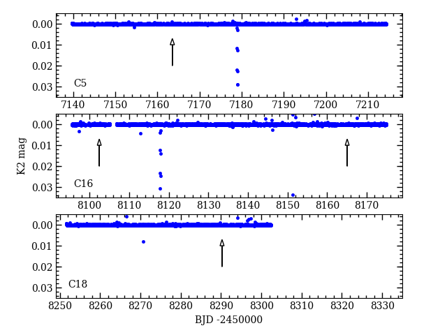
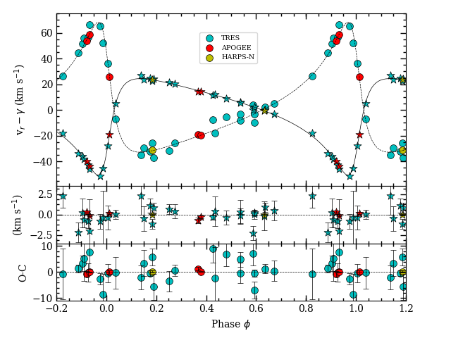
M67 was observed during Campaigns 5, 16, and 18 of the K2 mission. WOCS 11028 was observed during all of the campaigns in a custom aperture with long cadence (30 min) exposures. Single eclipses were observed during campaigns 5 and 16, having about a 2.7% decrease in flux. (No eclipse was observed in campaign 18 data, and the ephemeris indicates that one was not expected.) The eclipse times were measured to be at BJD , and using the bisector method of Kwee & van Woerden (1956). The radial velocity curve shows that these are secondary eclipses (of the cooler, less massive star). In the K2 light curves, there is no sign of primary eclipses at the four epochs predicted by the orbital ephemeris (see Figure 1).
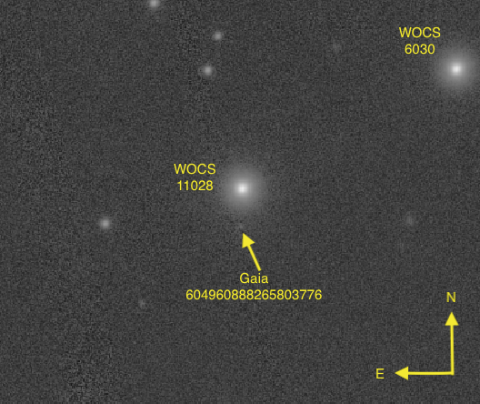
Because the K2 camera has relatively large pixels ( on a side), we briefly discuss the possibility of contaminating light from unrelated stars. Although WOCS 11028 is a member of M67, it is in the outskirts of the cluster. As shown in Figure 2, the nearest bright star is WOCS 6030 / Sanders 619 at a distance of , and about 0.3 mag fainter in Gaia band. There is a Gaia source (indicated in Figure 2) away, but nearly 8 magnitudes fainter. There are three other Gaia sources between 27 and away, but all are at least 5.3 mag fainter in . In the light curves described below, the photometric apertures did not extend more than 5 pixels away from the photocenter, and so avoided the brighter stars. As a result, we assume contamination of the K2 apertures used for WOCS 11028 is negligible.
Because of the incomplete gyroscopic stabilization during the K2 mission, systematic effects on the light curve are known to be substantial. We used two different light curves for WOCS 11028 as part of our investigation of systematic error sources. The first light curve we experimented with utilized the K2SFF pipeline (Vanderburg & Johnson, 2014; Vanderburg et al., 2016) that involved stationary aperture photometry along with correction for correlations between the telescope pointing and the measured flux. The light curve that resulted still retained small trends over the long term, so these were removed by fitting the out-of-eclipse points with a low-order polynomial and dividing the fit. The second light curve came from version 2.0 of the EVEREST pipeline (Luger et al., 2018), which uses pixel-level decorrelation to remove instrumental effects. We used the detrended and co-trending basis vector-corrected light curve. However, the eclipse depth is about 4% deeper in the EVEREST light curve than in the K2SFF version, so we need to gauge the effects on measurements of the binary characteristics. Because the K2 light curves have high signal-to-noise, they have a substantial influence on best-fit binary star parameter values (see section 3.4). The scatter among the best-fit parameter values when comparing runs with different K2 light curve reductions is sometimes larger than the statistical uncertainties. Because there is no clearly superior method for processing the K2 light curves, we will take the scatter in the binary model parameter values as a partial indicator of systematic error resulting from the processing.
2.2 The Spectral Energy Distribution
Because the eclipses of the WOCS 11028 binary provide minimal information on the sizes of the individual stars, we need other well-measured characteristics of the binary’s stars in order to extract age information for the cluster. Fortunately, M67 has been heavily observed over a wide wavelength range, making it possible to construct well-sampled spectral energy distributions for the binary and similarly bright stars in the cluster. In this section, we describe the spectroscopy and photometry we have assembled, and the efforts to put the observations on a consistent flux scale.
Ultraviolet: We obtained photometry and a spectrum from the Galaxy Evolution Explorer (GALEX; Martin et al. 2005) archive for the NUV passband ( Å). WOCS 11028 was imaged twice, for 1691.05 s (GI1 proposal 94, P.I. W. Landsman) and 5555.2 s (GI1 proposal 55. P.I. K. Honeycutt). As the archived magnitudes are based on count rates with minimal background contributions, we computed a final magnitude and flux based on the average count rate for both observations. Morrissey et al. (2007) describes the characteristics of the GALEX photometry and its calibration to flux. GALEX magnitudes are on an AB system (Oke & Gunn, 1983), and we used the zero point magnitude () and reference flux ( erg s-1 cm2 Å-1) to convert to flux.
A NUV grism spectrum was taken as part of GI1 proposal 94 (PI: W. Landsman) on 2005 Feb. 18 with a total exposure time of 27653 s. The NUV spectrum covers a wider wavelength range than the NUV photometry filter, but there was effectively no signal detected for WOCS 11028 at wavelengths less than about 2000 Å. The spectrum was obtained from MAST, and the flux calibration from the pipeline reduction was used.
Observations were taken of a smaller portion of M67 (including WOCS 11028) using the UVOT telescope on the Swift satellite. We collected UV fluxes in the , , and bands from the Swift UVOT Serendipitous Source Catalogue (version 1.1; Page et al. 2014). The three bands mostly cover the same wavelength range as the GALEX NUV filter, but with somewhat finer resolution. Flux correction factors from Poole et al. (2008) were applied to go from the gamma-ray burst spectrum calibration given in the archive to one utilizing Pickles (1998) library stars.
Near-ultraviolet, Optical and Near-infrared: M67 has been frequently observed from the ground for the purposes of photometric calibration. For the purposes of an SED, narrow-band filters are particularly useful, and we discuss these first. Balaguer-Núñez et al. (2007) presented Strömgren photometry for the cluster. Because M67 stars are commonly used as standards in Strömgren photometry (Nissen et al., 1987), we can be fairly assured that the observations are tied to the standard system. We employed reference fluxes from Gray (1998) to convert the magnitudes to fluxes.
Fan et al. (1996) conducted wide-field observations of M67 in a series of narrow-band filters (“BATC”) covering from 3890 to 9745 Å using bandpasses avoiding most important sky lines. The wavelength coverage of the filters is better in the near-infrared, making them a good complement to Strömgren photometry. The BATC survey goal was spectrophotometry at the 1% level, and the study largely achieved that, judging from the low scatter in their color-magnitude diagrams. Their reported magnitudes are on the Oke & Gunn AB system. We found that fluxes from these magnitudes were systematically higher than similar observations in other systems. We collected magnitudes in a larger set of filters from BATC Data Release 1111http://vizier.u-strasbg.fr/viz-bin/VizieR-3?-source=II/262/batc, and found that these were more consistent, probably due to improved calibration (Zhou et al., 2003).
Narrow-band photometry is also available in the Vilnius filter system for many stars in M67 (although not WOCS 11028) in the study of Laugalys et al. (2004). We converted the reported magnitudes to fluxes using the zeropoints from Mann & von Braun (2015). The filters in the Vilnius system are somewhat denser in the blue portions of the optical, and these again complement the spectrophotometry in the BATC system.
We have Johnson-Cousins photometry in from Sandquist (2004) and Yadav et al. (2008), in from Montgomery et al. (1993), in from Nardiello et al. (2016b), and in from Data Release 9 of the AAVSO Photometric All-Sky Survey (APASS; Henden et al. 2015). These measurements are on a Vega magnitude system, and so have been converted to fluxes using reference magnitudes from Table A2 of Bessell et al. (1998), and accounting for the known reversal of the zero point correction rows for and . The absolute calibrations of each of these studies are unavoidably different for the same filter bands, and this will contribute to the noise in the SEDs. However, this does not affect their use in determining the relative contributions of the two stars in the WOCS 11028 binary (see §2.2.1). (The and filter observations given in Nardiello et al. (2016b) were actually taken in SDSS and filters, and have been recalibrated to the Sloan DR12 system (D. Nardiello, private communication). These data were not used in fits to SEDs.)
There are several additional surveys that provide calibrated broad-band photometric observations. We used PSF magnitudes from Data Release 14 of the Sloan Digital Sky Survey (SDSS; York et al. 2000), calibrated according to Finkbeiner et al. (2016). The SDSS is nearly on the AB system, with small offsets in and that we have also corrected for here. The Pan-STARRS1 survey (Kaiser et al., 2010) contains photometry in 5 filters, and we use their mean PSF magnitudes here. Zero points for its AB magnitude system are given in Schlafly et al. (2012). The APASS survey also observed the cluster in Sloan filters, and their photometry was flux calibrated from the AB system.
Finally, Gaia has already produced high-precision photometry extending far down the main sequence of M67 as part of Data Release 2. We obtained the fluxes in the , , and bands from the Gaia Archive.
Infrared: We obtained Two-Micron All-Sky Survey (2MASS; Skrutskie et al. 2006) photometry in from the All-Sky Point Source Catalog, and have converted these to fluxes using reference fluxes for zero magnitude from Cohen et al. (2003). Many stars also have photometry in three bands from the Wide Field Infrared Explorer (WISE; Wright et al. 2010), which were also converted to fluxes using tabulated reference fluxes at zero magnitude.
2.2.1 Photometric Deconvolution
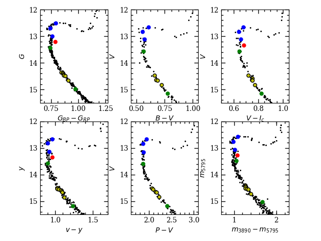
A benefit of the binary’s membership in the M67 cluster is that it should be possible to describe the binary’s light as the sum of the light of two single cluster stars. To that end, we compiled a database of photometric measurements from likely single main sequence stars in M67, and sought a combination of stars whose summed fluxes most closely match the fluxes of WOCS 11028. For our sample of probable single stars, we selected likely members based on Gaia proper motions, parallaxes, and photometry, as well as radial velocity membership and binarity information from Geller et al. (2015). Likely binaries were rejected by restricting the sample to those classified as radial velocity SM (single members) with Gaia photometry placing them within about 0.03 mag of the blue edge of the main sequence band in the color. Selected stars are shown in Figure 3.
The benefit of this procedure for constraining the SEDs of the binary’s stars is that it is a relative comparison using other cluster stars with the same distance, age, and chemical composition. As such, it is independent of distance and reddening (as long as these are the same for the binary and comparison stars), the details of the filter transmission curves (as long as the same filter is used for observations of the different M67 stars), and flux calibration of any of the filters (as long as the calibration is applied consistently). We can also avoid systematic errors associated with theoretical models or with the consistency of the different parts of empirical SEDs compiled from spectra.
We tested two ways of doing the decomposition: using actual M67 stars as proxies and checking all combinations of likely main sequence stars; and fitting all main sequence stars with photometry in a given filter as a function of Gaia magnitude in order to derive SEDs that could be combined. When using actual M67 stars, we are somewhat at the mercy of the photometry that is available for each star (and the binary) and of the stellar sampling of the main sequence. The use of fits allows for finer examination of the main sequence, although there is some risk of diverging from the photometry of real stars. Even for a relatively rich cluster like M67, parts of the main sequence are not well populated, and we believe that the main-sequence fitting method gives better results in that case. We present the results of both analyses below, however.
To judge the agreement between the summed fluxes of a pair of stars and the binary photometry, we looked for a minimum of a -like parameter involving fractional flux differences in the different filter bands:
where and is the magnitude uncertainty in the th filter band for the binary. The addition of 0.01 mag somewhat deweights photometry with very low uncertainties (Gaia and GALEX NUV) that results partly from their very wide filter bandpasses.
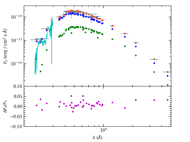
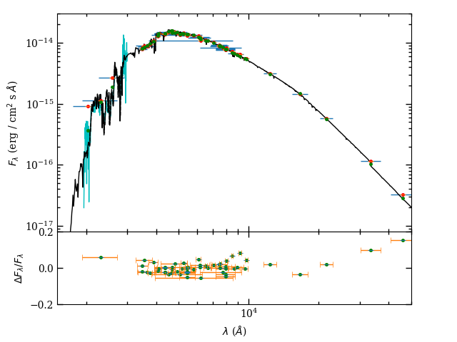
When using M67 stars as proxies, the results can be affected by the selection of filters that could be used. We examined solutions excluding the Swift/UVOT and/or Strömgren photometry because they covered the smallest portion of the cluster field, and excluding them allowed us to use larger sets of stars. The sample sizes were 52 stars having photometry in all of the filter bands, 109 with UVOT excluded, and 125 with UVOT and Strömgren photometry excluded. In all cases, the best fits involved WOCS 6018 (Sanders 763) as the brighter star, while the preferred fainter star was either WOCS 10027/S1597 (with UVOT photometry excluded) or WOCS 16013/S795 (for all photometry, or with UVOT and Strömgren excluded). Solutions involving WOCS 6018 with different faint stars (WOCS 17021/S820, WOCS 21046/S1731, WOCS 16018/S814) were the next-best fits, and all of these stars reside in similar positions on the main sequence. Figure 4 shows a comparison of the SED of WOCS 16013 with WOCS 6018, giving an indication of the significant optical and infrared excess for the binary. The bottom panel shows the residuals between the binary flux and the summed fluxes of WOCS 6018 and WOCS 10027. A potential limiting factor is the stellar sampling available near the brighter star, but we have stars within 0.007 mag on the bright side and within 0.016 mag on the faint side.
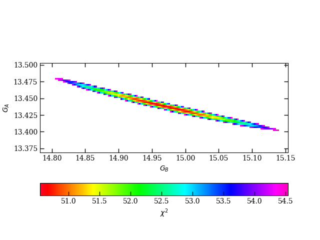
The main-sequence fitting procedure can be employed in any filter with a sufficient sample of stars covering the range of brightnesses for the binary’s stars. In our case, this eliminated the , Swift , and WISE W3 and W4 filters from consideration. Our fit statistic had a minimum value of 50.0 for the selection of 46 filters. We estimated the uncertainty in the fit based on where the goodness-of-fit statistic reached a value of 4 above the minimum value. For example, this returns and . As expected, there is an anti-correlation between values for the primary and secondary stars because of the need to match the binary fluxes (see Fig. 5).
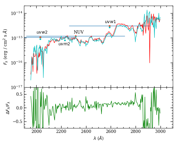
For an additional check on the brighter star, we compared the GALEX ultraviolet spectrum of WOCS 11028 with that of WOCS 6018, as shown in Fig. 6. Although our minimization procedure encourages agreement in near-UV filters, it doesn’t require agreement of the spectra. In spite of this, the overall shape and flux level of the two stars agree well, with the binary becoming consistently higher on the long wavelength end. The slope of the GALEX spectrum is one of the more sensitive indicators of temperature for stars on the upper main sequence of M67, and this combination of stars does a better job of reproducing that than two equal-mass stars, for example. The enhancement in flux at the long-wavelength end of the spectrum can be attributed to a small contribution from the faint star in the binary. The four photometric observations in the near ultraviolet (from GALEX and Swift/UVOT) indicate that the binary is slightly brighter than WOCS 6018 in all of the filter bands.
The above fits to the binary’s photometry provide luminosity ratios in different bands independent of models, and we use some of these as constraints in modeling the radial velocity and eclipse light curve data in §3.4. These ratios are provided in Table The K2 M67 Study: Precise Mass for a Turnoff Star in the Old Open Cluster M67.
2.2.2 Effective Temperatures and Bolometric Fluxes
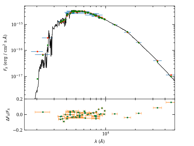
With SEDs in hand for stars that we believe are good proxies for the binary’s components, we can derive additional properties via fits with theoretical models. The models can introduce systematic errors in the quantities we try to measure, although we will try to mitigate them. We tested models from ATLAS9 (Castelli & Kurucz, 2004)222The models were calculated using the ATLAS9 fortran code that employed updated 2015 linelists, and at temperatures between the published gridpoints. and Coelho (2014), but the results were very similar, and we primarily discuss ATLAS9 model fits below. Models were adjusted to account for the interstellar reddening of M67 [; Taylor 2007] using the Cardelli et al. (1989) extinction curve. Model photometry was calculated using the IRAF333IRAF is distributed by the National Optical Astronomy Observatory, which is operated by the Association of Universities for Research in Astronomy (AURA) under a cooperative agreement with the National Science Foundation. routine sbands. Bolometric flux was derived from the median multiplicative factor needed to bring the best-fit model photometry into agreement with each observation, and we quote an uncertainty on the median that is based on the range covered by observations that are within entries of the middle in the ordered list. We find that the SEDs of WOCS 6018 and the bright component from our main sequence fit method are in good agreement with models of 6200 K (see Fig. 7), while all of the candidate fainter components indicate a temperature of about 5500 K (see Fig. 8).
To try to achieve greater precision, we also calculated temperatures using the infrared flux method (Blackwell & Shallis, 1977, IRFM;). Briefly, this method exploits the difference in temperature sensitivity between the bolometric flux and monochromatic fluxes in the infrared on the Rayleigh-Jeans portion of the spectrum. With the available photometry databases, we have measurements of fluxes covering the majority of the stellar energy emission. The ratio of the bolometric and infrared fluxes (we use fluxes in 2MASS bands) can be compared to theoretical values (where we again use ATLAS9 models):
We used the 2MASS flux calibration of Casagrande et al. (2010) in this case, in part because it produced greater consistency between the temperatures derived in the three bands — full ranges between 15 and 40 K. Starting from a solar-metallicity ATLAS9 model that produced a good fit by eye, we adjusted the temperature of the synthetic spectrum until it matched the average IRFM temperature from the three 2MASS bands. We find temperatures of 6185 K and 5500 K for the two stars. The model surface gravity was chosen from the eclipsing binary results or from MESA models, although changes had little effect. Uncertainty in the reddening (which modifies the shape of the theoretical model we fit to the data) and metal content of the models affects the measured temperature at about the 15 K level. Overall, we estimate that there is an uncertainty of about 50 K and 75 K in the temperatures.
For comparison, there are spectroscopic temperatures available for stars near the position of the brighter star in the CMD from recent surveys looking at abundance differences as a function of evolutionary phase. Liu et al. (2019) found temperatures by forcing excitation and ionization balance in their modeling of Fe I and II lines, and for three stars slightly brighter in , they derived temperatures between about 6100 and 6150 K. Souto et al. (2019) found temperatures from ASPCAP fits to infrared APOGEE spectra and the three closest stars in covered a range from 6050 to 6110 K (in their “calibrated” ASPCAP values). Gao et al. (2018) derived temperatures from fits to first and second ionization states of Sc, Ti, and Fe lines, and two H Balmer lines, and for the stars nearest in magnitude, they found a range from about 6090 to 6140 K. (Our best fit M67 star, WOCS 6018, had a temperature of 6127 K.) Bertelli Motta et al. (2018) used temperatures from the Gaia-ESO Survey, and observed four stars slightly fainter than WOCS 6018 that returned a range between 6000 and 6060 K. Önehag et al. (2014) derived temperatures from photometry, but also examined ionization and excitation temperatures. For five stars slightly fainter than our fit, they found temperatures between about 6130 and 6200 K, with the closest matches in brightness being at the high end of that range. The agreement of our IRFM temperature with these spectroscopic measurements is quite good, and if anything, our temperature is higher than spectroscopic values by K.
We can also derive bolometric fluxes at Earth from the model fits to the SEDs. The SEDs for both stars are very well sampled with photometry, and a GALEX spectrum for the best bright star proxy can be employed as well. The results are summarized in Table The K2 M67 Study: Precise Mass for a Turnoff Star in the Old Open Cluster M67. The SED model fits can be combined to provide a constraint on the radius ratio for the two stars that is independent of the distance and reddening of the cluster via
Because the single grazing eclipse per orbit gives us a constraint on the sum of the stellar radii, this radius ratio will allow us to compute the individual stellar radii.
2.3 Spectroscopy
We have measured radial velocities for the WOCS 11028 binary using three spectroscopic datasets. The first and largest set we employ here comes from the CfA Digital Speedometers (Latham, 1985, 1992) on the 1.5 m Tilinghast reflector at Fred Lawrence Whipple Observatory and the MMT. These observations were recordings of a single echelle order covering 516.7 to 521 nm around the Mg I b triplet using an intensified photon-counting Reticon detector. The spectra were taken as part of a larger monitoring campaign of M67 stars.
We made two observations of the binary using the HARPS-N spectrograph (Cosentino et al., 2012) on the 3.6 m Telescopio Nazionale Galileo (TNG). HARPS-N is a fiber-fed echelle that has a spectral resolving power , covering wavelengths from 383 to 693 nm. The spectra were processed, extracted, and calibrated using the Data Reduction Software (version 3.7) provided with the instrument.
We also obtained five archival spectra from the APOGEE database (Holtzman et al., 2015) that were taken between January and April 2014. These are -band infrared (m) spectra with a spectral resolution taken on the 2.5 m Sloan Foundation Telescope. We used APOGEE flags to mask out portions of the spectrum that were strongly affected by sky features, and continuum normalized the spectra using a median filter.
The radial velocities were measured using the spectral separation algorithm described in González & Levato (2006). In the first iteration step, a master spectrum for each component is isolated by aligning the observed spectra using trial radial velocities for that component and then averaging. This immediately de-emphasizes the lines of the non-aligned stellar component, and after the first determination of the average spectrum for each star, the contribution of the non-aligned star is subtracted before the averaging in order to better clean each spectrum. The radial velocities can also be remeasured from spectra with one component subtracted. This procedure is repeated for both components and continued until a convergence criterion is met. We measure the broadening functions (Rucinski, 2002) to determine the radial velocities using narrow-lined synthetic spectra as templates. Radial velocity measurements from broadening functions improve accuracy in cases when the lines from the two stars are moderately blended (Rucinski, 2002).
The CfA spectra covered a wide range of orbital phases that made it possible to use a large number of spectra in calculating average spectra for the two stars. In most cases, spectra were left out due to low signal-to-noise ratio. We used 17 out of 28 spectra in determining the average spectrum for the primary, but only used the 13 spectra with the most clearly detected secondary component to determine its average spectrum. With good average spectra, it was possible to subtract each component out of observed spectra even when they were taken close to crossing points (phases and 0.6). After some experimentation, we found that synthetic templates (from the grid of Coelho et al. (2005)) of 5250 K optimized the detection of broadening function peaks for the secondary star. A template with 6250 K was used for the primary star. For the CfA velocities only, we used run-by-run corrections derived from observations of velocity standards. Run-by-run offsets measured for the CfA spectra ranged from to km s-1. We initially assigned velocity uncertainties derived from the spectral separation analysis, but scaled these to ensure that the scatter around a best-fit model for this dataset was consistent with the measurement errors. (In other words, we forced the reduced value to 1.) The average uncertainty for the primary star velocities was 1.25 km s, and for the secondary star it was 4.41 km s-1.
The APOGEE spectra were analyzed separately, and detection of the secondary star features were considerably more secure. The synthetic spectral templates were taken from ATLAS9/ASST models (Zamora et al., 2015) calculated for the APOGEE project. The uncertainty estimate for each APOGEE velocity was generated from the rms of the velocities derived from the three wavelength bands in the APOGEE spectra. This was typically around 0.15 km sfor the primary star and 0.65 km sfor the secondary star. The velocity was corrected to the barycentric system using values calculated by the APOGEE pipeline. For all five spectra, the broadening function peaks for the two stars were resolvable thanks to the high resolution of the spectra and fortuitous phases of observation.
Because we only had two observations using the HARPS-N spectrograph and one of them was taken at a phase very near a crossing point, we determined velocities using broadening functions alone. To get an internal measure of the velocity uncertainties, we measured the velocities in four 30 nm subsections of the spectra and computed the error in the mean.
Because the synthetic spectra used in our broadening function measurements do not account for gravitational redshifts of the stars, our velocities should have an offset relative to velocities derived using an observed solar template. For the CfA spectra, the run-by-run corrections were computed using dawn and dusk sky exposures, and this defines the native CfA velocity system used in Geller et al. (2015), incorporating the gravitational redshift of the Sun. For consistency, we subtracted the combined gravitational redshift of the Sun and gravitational blueshift due to the Earth (0.62 km s-1) from the APOGEE and HARPS-N velocities we tabulate. Based on the derived masses and radii for the stars in the binary, they should have slightly larger gravitational redshifts than the Sun (0.66 and 0.69 km s-1, versus 0.64 km sfor the Sun) but we did not correct for these smaller differences. In our later model fits, we did, however, allow the system velocities for the two stars to differ to account for effects like this and convective blueshifting that could produce small systematic shifts. These could affect the measured radial velocity amplitudes and (and the stellar masses) if not modeled.
The measured radial velocities are presented in Table 1, and the phased radial velocity measurements are plotted in Fig. 9. The model fits are described in Section 3.4, but the parameters that were used to fit the velocity data were the velocity semi-amplitude of the primary star , mass ratio , eccentricity (), argument of periastron (), and systematic radial velocities and . In the end, we do not see noticeable differences between the systematic velocities.
| mJDaamJD = BJD - 2400000. | mJDaamJD = BJD - 2400000. | ||||||||
|---|---|---|---|---|---|---|---|---|---|
| (km s-1) | (km s-1) | (km s-1) | (km s-1) | ||||||
| CfA Observations | 49678.02714 | 54.71 | 0.59 | 6.53 | 3.23 | ||||
| 48347.73537 | 3.84 | 98.95 | 6.47 | 49700.00054 | 38.07 | 0.89 | 29.41 | 2.87 | |
| 48618.00088 | 53.87 | 0.59 | 0.83 | 3.95 | 49705.98524 | 31.68 | 1.77 | ||
| 48635.87968 | 38.55 | 1.48 | 24.19 | 3.95 | 50535.69747 | 1.18 | 76.62 | 1.44 | |
| 48676.79118 | 56.54 | 0.59 | 5.03 | 50536.76047 | 1.77 | 84.15 | 2.87 | ||
| 48701.71198 | 32.68 | 0.89 | 36.16 | 4.67 | 50885.78158 | 41.13 | 0.89 | 27.03 | 4.67 |
| 48704.66488 | 32.50 | 0.59 | 34.70 | 1.80 | 50913.75637 | 0.89 | 88.80 | 3.59 | |
| 48726.74348 | 3.25 | 84.47 | 7.90 | 50916.72187 | 0.89 | 97.47 | 2.16 | ||
| 48754.67588 | 44.44 | 1.77 | 14.28 | 11.86 | 50918.72237 | 4.69 | 1.48 | 68.75 | 3.59 |
| 48942.01949 | 44.13 | 0.30 | 25.07 | 5.39 | 50920.71047 | 37.55 | 0.59 | 25.23 | 6.11 |
| 48966.93949 | 14.32 | 1.48 | 58.96 | 9.70 | APOGEE Observations | ||||
| 48988.95240 | 57.20 | 0.89 | 1.08 | 56672.86368 | 0.06 | 91.22 | 0.09 | ||
| 49019.89560 | 29.34 | 1.18 | 37.60 | 3.95 | 56677.88083 | 13.45 | 0.15 | 57.87 | 0.64 |
| 49049.81820 | 56.23 | 1.48 | 3.07 | 5.03 | 56700.76762 | 46.59 | 0.15 | 12.91 | 0.17 |
| 49057.71970 | 52.50 | 0.89 | 6.60 | 2.16 | 56734.66627 | 0.13 | 85.78 | 1.07 | |
| 49077.68900 | 34.51 | 0.59 | 29.15 | 1.44 | 56762.63514 | 46.73 | 0.35 | 13.13 | 0.64 |
| 49111.72870 | 59.12 | 2.36 | 4.67 | HARPS-N Observations | |||||
| 49328.01792 | 34.75 | 0.30 | 22.47 | 3.23 | 57752.76085 | 55.83 | 0.08 | 1.04 | 0.30 |
| 49347.86222 | 0.89 | 88.10 | 8.62 | 57780.74729 | 31.82 | 0.03 | |||
It is always prudent to check for systematic differences in velocity when utilizing datasets from more than one observational set-up. Among the measured primary star velocities, mean residuals (observed minus computed) were km sfor APOGEE, km sfor CfA, and km sfor HARPS-N. For the secondary star, we found mean residuals of km sfor CfA, km sfor APOGEE, and km sfor HARPS-N (one measurement). Of these, only the average residual for the CfA secondary velocities was more than one standard devation (0.20 km s-1) away from zero. Because the APOGEE and HARPS-N spectra have higher signal-to-noise than the CfA spectra, they are the main contributors to measurement of the radial velocity amplitude of the secondary star, which critically affects the calculated mass of the primary star.
3 Analysis
3.1 Cluster Membership
WOCS 11028 is a fairly large distance (about ) from the center of M67, but Carrera et al. (2019) find that half of the cluster turnoff stars fall within of the cluster center. As a result, its position is not strong evidence of being a field star.
All ground-based proper motion studies (Sanders, 1977; Girard et al., 1989; Zhao et al., 1993; Yadav et al., 2008; Nardiello et al., 2016a) indicate a high probability (%) of cluster membership for WOCS 11028, with the exception of Krone-Martins et al. (2010), who give 10%). Gaia observations from Data Release 2 (Gaia Collaboration et al., 2018a) have produced much more precise proper motions recently, and the binary still has a proper motion vector ( mas yr-1, mas yr-1) safely residing among other likely members (centered at mas yr-1, mas yr-1; Gaia Collaboration et al. 2018b). Similarly, the Gaia parallax ( mas) is within of the cluster mean ( mas).
Geller et al. (2015) published membership probabilities based on their radial velocity survey by comparing the velocity distributions of cluster members and field stars. They classified WOCS 11028 as a binary member (98% probability) based on their system velocity ( km s-1) measured from the CfA observations and carefully placed on the zeropoint of other stars in the field. The best-fit system velocity from our measurements ( km s-1) is slightly off from the mean cluster velocity of Geller et al. (33.64 km swith a radial velocity dispersion of km s-1). However, even with our lower velocity, the radial velocity membership probability is still 95%.
Based on the three-dimensional kinematic evidence, the binary is a high probability cluster member.
3.2 Distance Modulus
With the release of Gaia DR2 parallaxes, the M67 distance modulus should be revisited, as it will play a large role in comparisons with models later in the article. The mean parallax derived for cluster members from Gaia DR2 measurements ( mas; Gaia Collaboration et al. 2018b) is very precise, but possibly affected by a zeropoint uncertainty. Lindegren et al. (2018) finds an offset of about as (with tabulated parallaxes being smaller than reality), while systematic variations with position, magnitude, and color were below as. At the other extreme, Stassun & Torres (2018) found an offset of as using a sample of eclipsing binaries. Zinn et al. (2019) find offsets of and as using comparisons with asteroseismic giants and red clump stars in the Kepler field. Schönrich et al. (2019) derived an offset of as from an analysis of all stars (more than 7 million) in the radial velocity sample of Gaia DR2.
These indications are consistent with the situation for M67. Without correction, the Gaia cluster mean distance modulus would be , but this is comparable to what has been derived previously for the distance modulus with extinction. For example, Pasquini et al. (2008) derive (statistical and systematic uncertainties) from ten solar analogs, Sandquist (2004) derived using metal-rich field dwarfs with Hipparcos parallaxes, and Stello et al. (2016) found from K2 asteroseismology of more than 30 cluster red giants. With a -band extinction expected, this is a significant discrepancy. For subsequent calculations in this article, we will assume a as offset in the Gaia parallaxes and include a systematic uncertainty of as to conservatively account for disagreement in the parallax offsets in the literature. The resulting distance modulus is .
3.3 Li Abundance and Stellar Rotation
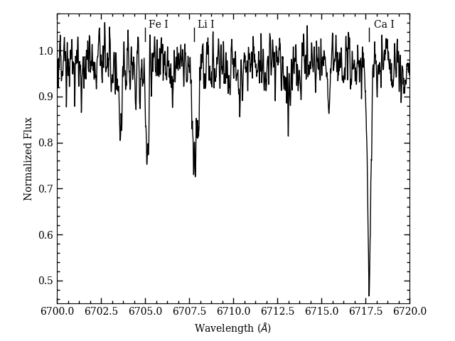
Even though the WOCS 11028 binary has a relatively large orbital separation, our analysis of another wide binary in M67 (WOCS 12009; Sandquist et al., 2018) indicated that the brighter star was likely the product of an earlier merger. A key piece of evidence for that binary was the lack of detectable Li. Single main sequence stars of similar brightness in the cluster inhabit the Li plateau, a broad maximum in the Li abundance. The lack of detectable Li was an indication of nuclear processing, consistent with surface material having originally been in a lower-mass main sequence star with a deeper surface convection zone.
To have greater assurance that the stars of WOCS 11028 have evolved as isolated single stars and can be used to constrain the cluster age, we can also use the Li abundance here. If the brighter star in WOCS 11028 was unmodified since the cluster’s formation, its mass () would place it toward the bright end of the cluster’s Li plateau with abundances (Pace et al., 2012). On the other hand, the secondary star (mass near ) should not have detectable Li. Stars in the plateau have outer convective zones that do not transport Li nuclei down to temperatures where nuclear reactions can burn them, and additional mixing processes must have little, if any effect. Even with the diluting effects of the secondary star’s light on the Li lines, Li should be detectable if it is present with the plateau abundance.
We are able to detect Li in our HARPS-N spectra as shown in Fig. 10. If the star had a history of interaction (mass transfer, or a merger involving lower mass stars), it is unlikely that the Li would be detectable. If the brighter star formed in a merger, the more massive merging star could not have been more than about less massive than the current star or else a surface convection zone would have had a chance to consume its Li during its main sequence evolution. In addition, the less massive merging star would take up residence in the core of the merger remnant because of its lower entropy, rebooting its nuclear evolution with gas having higher hydrogen abundance. After some adjustment on a thermal timescale, it would have been bluer than other cluster stars of the same mass. A precise determination of the Li abundance is complicated by the secondary star’s light, and is beyond the scope of this work. However, the strong Li detection coupled with strong indications that WOCS 11028 A has a color consistent with its fellow cluster members effectively rules out anything except a very early merger and/or a merger with a very low mass object. Effectively, this would make today’s star the same as an unmodified star of the same mass.
We do not see evidence of rotational spot modulation in the K2 light curves due to spots, but our HARPS-N spectra allow us to constrain the rotational speeds of the stars in the binary via the widths of the broadening function peaks. We are unable to detect rotation with an upper limit km s-1. If the primary was pseudo-synchronized, its rotation velocity would be around this limit (rotation period near 14 d). However, the timescale calculated for this (Hut, 1981) is far longer than the cluster age, thanks to the substantial separation even at periastron. Considered as a single star, the primary has probably spun down somewhat, although not to the same degree as lower mass stars with deeper surface convection zones. Angus et al. (2015) calibrated their gyrochronological models against the rotation of asteroseismic targets in the Kepler field, and their sample probably gives the best indication of typical rotation rates for old stars more massive than the Sun. Their isochrones predict a rotation period near 16 day, and this would imply a rotation velocity below our ability to detect it spectroscopically. As an old cluster, M67 is expected to have slowly rotating stars, but this does put a limit on how long ago mass transfer or a merger could have happened if either star was somehow modified. A rapidly rotating star with the mass of our primary star would require approximately 3 Gyr to reach our detection limit according to the rotational isochrones of Angus et al. (2015), and this is the majority of the cluster’s age.
3.4 Binary Star Modeling
We used the ELC code (Orosz & Hauschildt, 2000) to simultaneously model the ground-based radial velocities and Kepler K2 photometry for the WOCS 11028 binary. The code is able to use a variety of optimizers to search the complex multi-dimensional space of parameters used in the binary star model. In our particular case, we used a set of 15 parameters. Two of the parameters were the orbital period , and the reference time of periastron . Six additional parameters mostly characterize the orbit: the velocity semi-amplitude of the primary star , mass ratio , systematic radial velocities444We allow for the possibility of differences for the two stars that could result from differences in convective blueshifts or gravitational redshifts. and , eccentricity (), and argument of periastron (). For a typical double-lined spectroscopic and eclipsing binary, both the radial velocities and eclipse light curves constrain and , with the phase spacing of the eclipse playing a large role. But because this binary only has one eclipse per cycle, these parameters are constrained by the radial velocities almost exclusively.
The light curve has a large role in constraining the inclination parameter , but there are potentially correlations between inclination and choices for radius and temperature parameters. For radii, we used the sum of the stellar radii and their ratio as parameters. For this binary, the sum of radii is constrained by the measurements of the single grazing eclipse in each cycle along with the well-determined spectroscopic parameters of the orbit. The radius ratio can be constrained by luminosity ratios we have derived from our SED analysis (§2.2) in concert with temperature information. For a typical eclipsing binary, the temperature ratio would be constrained by the relative depths of the eclipses, but that is not measurable here. We have separate constraints on the temperatures of the stars from SED fits to the proxy stars, and so we use these as fit parameters: temperatures of the primary and secondary .
Finally, there is some dependence of the fits on the limb darkening, although relatively little because only the near-limb of the secondary star is probed by the grazing eclipses we see. So we fit for two quadratic limb darkening law coefficients () for the secondary star (the only star that is eclipsed) in the Kepler bandpass. Our runs of the ELC code employed the Kipping (2013) algorithm, which involves a search over a triangular area of parameter space of physically realistic values. This forces the model star to a) darken toward the limb, and b) have a concave-down darkening curve. In the final analysis, we find that the limb darkening coefficients are virtually unconstrained, but by allowing the code to systematically explore potential values, the uncertainties will be incorporated in our uncertainties of the other stellar parameters. Owing to the substantial orbital separation, we assumed that the stars are spherical. Given this, we used the algorithm given in Short et al. (2018) as implemented in ELC to rapidly compute the eclipses. Finally, because there is little or no out-of-eclipse light modulation, we did not see a need to model spots.
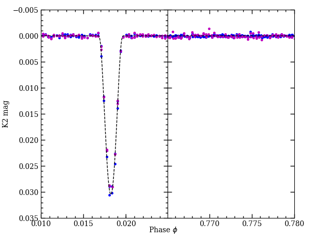
For the K2 light curve modeling, we only included observations that were within about in phase of the eclipse, and a similar section around where the other eclipse would have been if the binary was closer to edge-on. In this way, our models “see” that there is only one eclipse per orbital cycle. In doing this, we leave out the majority of observations, which may be affected by systematics due to spacecraft pointing corrections and other instrumental signals. Because the K2 light curves use long cadence data with 30 minute exposures, they also effectively measure the average flux during that time. To account for this, the ELC code integrates the computed light curves in each observed exposure window.
The quality of the model fit was quantified by an overall derived from comparing the radial velocity and light curve data to the models, as well as from how well a priori constraints were matched. For this binary, we used stellar temperatures derived from SED fits and luminosity ratios in derived from the modeling of the binary SED with single cluster stars. To illustrate the effect of these constraints, we conducted a run without the luminosity ratios, as shown in Table 2.
To try to ensure that different datasets were given appropriate weights in the models, we empirically scaled uncertainties on different datasets to produce a reduced of 1 relative to a best-fit model for that particular dataset. For spectroscopic velocity measurements, this meant scaling differently according to the source spectrograph and the star (primary and secondary). The K2 photometric light curve uncertainties were scaled independently.
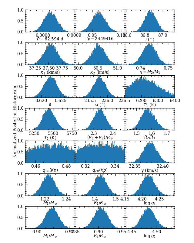
We used a differential evolution Markov Chain optimizer (Ter Braak, 2006) for seeking the overall best-fit model and exploring parameter space around that model to generate a posterior probability sampling. Approximate parameter uncertainties were derived from the parts of the posterior distributions containing 68.2% of the remaining models from the Markov chains. Gaussians were good approximations to the posterior distributions for all parameters except limb darkening coefficients in the run where luminosity constraints were applied. The results of the parameter fits are provided in Table 2, and the posterior distributions are shown in Figure 11. A comparison of the K2 light curve with the best-fit model is shown in Figure 12, and a comparison of the radial velocity measurements with models are shown in Figure 9.
| Parameter | No SED Constraint | SED Luminosity Constraints | |
|---|---|---|---|
| Pipeline | K2SFF | K2SFF | EVEREST |
| Constraints: | |||
| (K) | |||
| (K) | |||
| (km s-1) | |||
| (d) | 62.59484 | 62.59484 | 62.59482 |
| (d) | 0.00003 | 0.00003 | 0.00002 |
| 49416.060 | 49416.058 | 49416.061 | |
| 0.013 | 0.012 | 0.012 | |
| () | |||
| () | |||
| (km s-1) | |||
| (km s-1) | |||
| (cgs) | |||
| (cgs) | |||
As can be expected, when we do not enforce luminosity ratio constraints from SED fitting, there is no information on the ratio of radii in the data, and as a result, the radii of the stars are very poorly constrained. The mass determinations are essentially unaffected, however, because that information is contained in the radial velocity curves and the orbital inclination (derived from the light curve).
4 Discussion
M67 has long been studied because of similarities in chemical composition and age with the Sun, but stars at the cluster turnoff are approximately 20-30% more massive than the Sun, with substantial differences in internal physics. Stars with masses of may generate convective cores late in their main sequence evolution, and this plays a critical role in their evolution.
In the discussion below, we will leverage new information from two sources — precise measurements of the stars in the WOCS 11028 binary, and additional characterization of stars around the turnoff of the cluster — to identify conflicts with models, and to try to understand the physics that might be causing those conflicts.
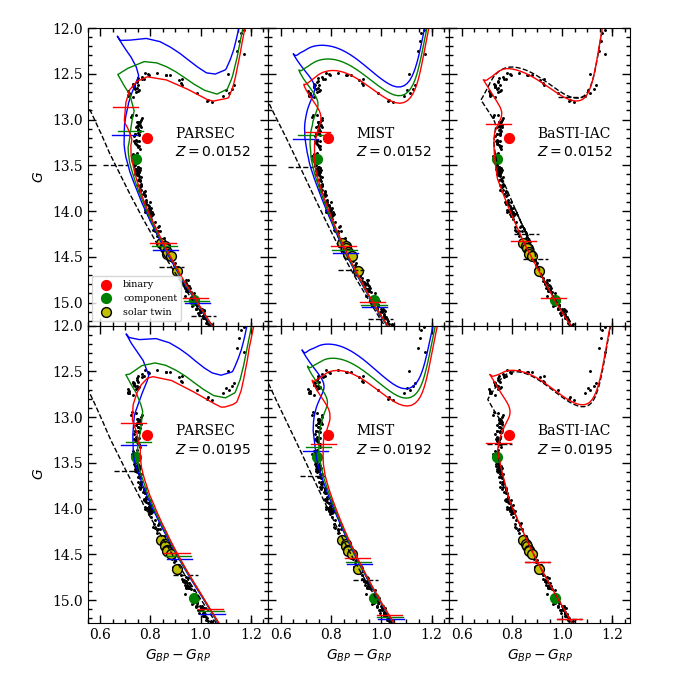
For clarity in the discussion, we define the upper turnoff to be at the global minimum in color at the blue end of the subgiant branch (); the turnoff gap slightly fainter than this (); and the lower turnoff to be at the fainter local color minimum (). Because WOCS 11028 A is nearly exactly at the lower turnoff based on our SED decomposition (see Figure 13), it provides an excellent mass calibration point for the cluster.
4.1 The Cluster Composition
As is usually the case, the chemical composition is an important component of interpreting the measurements and understanding the implications for the cluster age and for the stellar physics in the models we use. We discussed high-precision cluster [Fe/H] measurements relative to the Sun in Sandquist et al. (2018) in order to minimize systematic errors due to composition. Since that paper though, it has become clearer that diffusion is playing a role in the measured surface compositions of M67 stars. Significant trends in abundance are seen as a function of the evolutionary state of the stars, with subgiants having higher measured abundances than turnoff stars (Önehag et al., 2014; Bertelli Motta et al., 2018; Liu et al., 2019; Souto et al., 2019). Because subgiants should have deep enough convection zones to homogenize surface layers that were affected by heavy element settling, the subgiant abundances should be more representative of the initial bulk heavy element composition of the stars. The spectroscopic studies generally come to the conclusion that initial composition of the cluster members was [Fe/H] to . In the model comparisons below, we will consider initial metal compositions between solar and [Fe/H].
4.2 The Characteristics and Evolution Status of WOCS 11028 A and B
The verticality of the cluster CMD at the position of WOCS 11028 A constrains the present direction of its evolution track, and we illustrate the discussion with MESA model tracks (version r11701; Paxton et al. 2011, 2013, 2015, 2018, 2019) in the largest panel of Figure 14. The models predict that for the first 2 Gyr of the star’s life, it was evolving mostly upward in luminosity, with slowly increasing temperature before hitting a maximum and starting to decrease. The star must have started evolving more rapidly toward cooler temperature in order to change the local slope of the main sequence isochrone from increasing temperature to constant temperature with increasing mass. Comparing the markers showing common age for three stars of slightly different mass, the triplet becomes vertical near the midpoints of the tracks during this coolward movement. For greater age, the triplets have decreasing temperature with higher mass, and in M67 this corresponds to stars between the lower turnoff and the faint end of the gap.
The precise point where the vertical slope is produced will depend on details of the fuel consumption in this phase, but we can be assured that the star must still be evolving faster toward lower temperature than slightly lower mass stars (in other words, accelerating) or else it would not be able to match the temperature of those stars that should be evolving at a very similar speed. This in turn assures us that convection must be present in the core of the star — low-mass stars that do not establish convective cores on the main sequence only accelerate toward lower temperature when they are past central hydrogen exhaustion while on the subgant branch. So the mass measurement for WOCS 11028 A gives us an observational lower limit for stars that establish convective cores on the main sequence.
In the evolution tracks, the turn toward lower temperature occurs when the extent of the convective core increases in the latter half of core hydrogen burning. The CNO cycle overtakes the chain as the dominant energy generating reaction network while central temperature increases and hydrogen abundance declines. So not only do we have good measurements of the WOCS 11028 A star (described below), but we have an indication of physical conditions occuring within the star. A complete model of the star would match all of the measurements and evolutionary constraints with a unique set of parameters, while mismatches would indicate systematic errors.
4.2.1 Mass and Radius
Although the radii we derive from our analysis of the binary are not as precise as they could have been if the system had been doubly eclipsing, they can still provide some indication of the age independent of other stars in the cluster if the stars have not undergone mass transfer or mergers in their history555The more massive star in the binary WOCS 12009, analyzed in Sandquist et al. (2018) and mentioned in section 3.3, had a much smaller radius than expected for reasonable cluster ages, providing support for the idea of a stellar merger in that case. The radius of the less massive star may not have been involved in the merger, but its radius is also unlikely to be significantly different even if it was.. In addition, these comparisons are independent of uncertainties in quantities like distance and reddening.
The comparison with several sets of solar-metallicity isochrone models is shown in Figure 15. Taken at face value, WOCS 11028 A is smaller than predicted for typically quoted M67 ages ( Gyr) by or more, and WOCS 11028 B is larger than reasonable models by a similar amount. Note that if we are systematically underestimating the luminosity ratio used in our binary star modeling (as one might wonder from the discussion of the SED fits in §2.2), this would exacerbate the conflict with models by decreasing the primary star radius and increasing the secondary star radius.
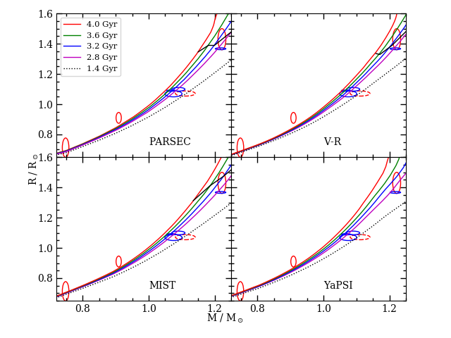
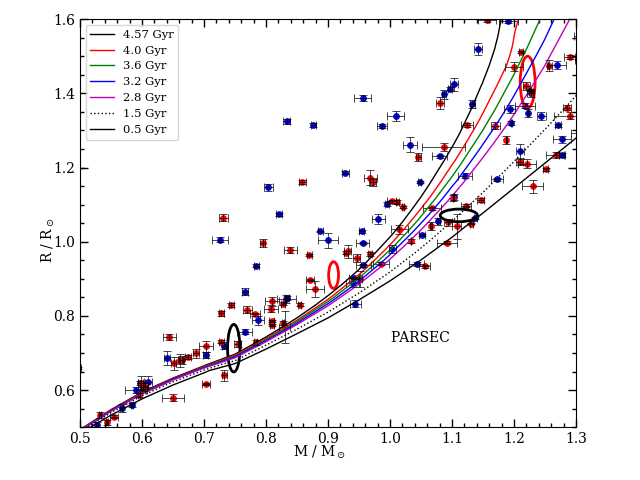
When compared with stars from well-measured binaries (Southworth 2015; see Figure 16), the secondary stars of the two measured M67 binaries (WOCS 11028 B and WOCS 12009 B) do not look out of the ordinary. PARSEC models generally underpredict radii for stars with like WOCS 11028 B, and this is not sensitive to the assumed age or metal content . The disagreement with models leads to some justifiable concerns whether a model age can be trusted if the characteristics of the relatively unevolved stars cannot be predicted accurately.
Among the stars in the Southworth (2015) sample are several from the younger but similarly metal-rich cluster NGC 6819 ( Gyr; Brewer et al., 2016). One of the stars is WOCS 40007 A, which has a mass () that is nearly identical to that of WOCS 11028 A. As another indicator of M67’s relative age, WOCS 11028 A is at M67’s turnoff, while WOCS 40007 A is approximately 0.85 mag fainter than NGC 6819’s turnoff in . WOCS 40007 A has a radius () that is smaller than WOCS 11028 A, although WOCS 11028 A’s radius is measured with about 10 times lower precision. So while WOCS 11028 A appears to be somewhat small relative to the model expectations for M67’s age, it does appear to be larger and older (by about 0.4 Gyr) than the corresponding stars of NGC 6819.
An absolute determination of the age requires comparisons to models though, and the characteristics of WOCS 11028 A return a value of Gyr for isochrones having . Radius is fairly insensitive to one of the more important model uncertainties — bulk metal content — and so should be given extra attention in considering the age. From experiments with MESA models, we find that for stars near WOCS 11028 A’s mass, whereas . By the same token, helium abundance generally affects radius in the opposite direction, and if one assumes, as most isochrone sets do, that galactic chemical evolution increases and together (in other words, is a constant), radius appears even less sensitive to composition changes. We will return to this point in Section 4.2.3.
We should also consider the evolutionary status of the brighter star WOCS 11028 A though. If models agree with our mass-radius measurements at a particular age but have the star at the wrong evolutionary state, it would be an indication of a systematic error in model physics. In Figure 15, we have connected isochrone points corresponding to the lower turnoff at each age. We find that, for all of the model sets we could check, the mass-radius combination for WOCS 11028 A is consistent with model predictions for that evolutionary stage.
4.2.2 The Color-Magnitude Diagram (CMD)
To date, the primary method for measuring the age of M67 has been isochrone fits to the CMD. Examples of results include 3.5 Gyr to 4.0 Gyr (Sarajedini et al., 2009) and 3.6 to 4.6 Gyr (VandenBerg & Stetson, 2004). A large portion of these age ranges result from model physics and chemical composition uncertainties that impact this cluster, and new information may help reduce the age uncertainty by reducing these modeling uncertainties. For example, Stello et al. (2016) used an asteroseismic analysis of the masses of pulsating giants in M67 to derive an age of about 3.5 Gyr, although that age still has uncertainties due to model physics.
The modeling of the eclipsing binary star gives us very precise masses for the component stars, and our SED analysis places restrictions on the CMD positions of the stars. These are the most precise data that can be extracted from the binary at present. When utilized with precise photometry for other cluster members, isochrone fitting can provide us with an estimate of the age. It is important to remember that masses are generally unavailable for traditional CMD isochrone fitting, and by employing them here, we can start to address systematic uncertainties on the derived age.
The Gaia photometric dataset is one of the most precise available, so in Figure 13 we compare the M67 photometry with theoretical isochrones. The isochrones were shifted based on the mean Gaia parallax for the cluster corrected for the Schönrich et al. (2019) zeropoint offset [for a distance modulus ), along with the Taylor (2007) reddening for the cluster [giving extinction and ]. The comparison indicates that the position of the faint component of WOCS 11028 is consistent with the theoretical predictions for its mass, especially considering an uncertainty in of about mag (see section 2.2). There is significant disagreement between the position of WOCS 11028 A and the model predictions for its mass, however. The theoretical predictions are at least about 0.17 mag too bright for the youngest models under consideration, and closer to the brightness level of the binary. It should be remembered as a practical matter that the magnitude of the brighter star is much more certain than the fainter star because of the need to match the brightness constraint of the binary, assuming that both stars are radiating like normal single star cluster members. Our earlier analysis puts the fit uncertainty at around mag in , so that an explanation beyond statistical uncertainty seems necessary.
The fact that model predictions fall near or brighter than the combined brightness of the binary reduces the range of possible explanations: either our assumption that the binary’s individual stars are emitting like unmodified single main sequence stars is wrong (and the binary’s light should not be modeled using stars on the main sequence), or there is a significant systematic error with model predictions. We have not seen any evidence to support the idea that the primary star is different from similar main sequence stars: there is detectable Li and the rotational velocity is low and consistent with a normally-evolving single star (section 3.3), and the ultraviolet emission from the binary can be reproduced very well by the emission of other cluster main sequence stars (section 2.2.1 and Figure 6). If the primary star had been modified earlier in its history, it should appear fainter and bluer than single main sequence stars that evolved uneventfully with the cluster.
We can also compare with stars from field eclipsing binaries having well-measured luminosity ratios in common filter bands. For this purpose, we examined stars from the DEBCat database (Southworth, 2015) with stellar masses within about of that of WOCS 11028 A, and kept those stars with precise Gaia parallaxes. The stars in our comparison are given in Table 5, and a comparison of the absolute magnitudes is shown in Figure 17. WOCS 11028 A is generally at the bright end of the range covered by stars with the most similar masses, which is to be expected given the age of the cluster it resides in. Even so, its magnitudes are quite comparable to several other stars: UX Men A and WZ Oph A and B agree extremely well with WOCS 11028 A in Strömgren filters, and WOCS 40007 A from the cluster NGC 6819 agrees quite well in magnitudes if we make use of a distance modulus derived from the eclipsing binaries in the cluster (as it is too distant for a good Gaia parallax). We conclude that WOCS 11028 A is not unusually faint for its mass, and this cannot explain the disagreement with model isochrones.
4.2.3 Temperature and Luminosity
With the variety of photometric measurements made for M67 stars, the SEDs provide us with excellent leverage on the temperatures of the binary star components as well as other cluster stars for comparisons. We find that both components of the binary agree well with stars from the DEBCat database, and the temperature of the primary star matches well with spectroscopic temperatures (see §2.2.1). While WOCS 11028 B matches the model temperature for its mass (see Figure 18), WOCS 11028 A is generally around 100 K cooler than the model that has its lower turnoff at the appropriate mass.
We can compute the luminosities for the stars in two different ways. The first uses the bolometric flux derived from SED fitting along with the Gaia-based distance and the inverse square law. The bolometric flux is computed assuming that any flux that is not covered by photometric measurements can be accounted for using an appropriate synthetic spectrum. The luminosities are found to be and for the proxies of the two stars in the binary. The quoted uncertainties include contributions from the parallax and the bolometric flux fit. Alternately, we can compute luminosities from the radii derived in the binary star analysis and the temperatures derived from the SED fits. Here the results are and , respectively. These estimates are marginally consistent with the values computed from the bolometric fluxes, but are less precise.
As seen in Figure 19, WOCS 11028 B is in general agreement with model luminosity predictions at solar metallicity, but WOCS 11028 A is about 25% lower than model values. This is a stronger statement than it might seem at first because we have the additional constraint on the evolutionary state of WOCS 11028 A. While it is possible to find a match with the models in luminosity and mass, this occurs at young ages when a star of WOCS 11028 A’s mass is not precisely at the lower temperature maximum at the cluster turnoff in the cluster CMD (see §4.2). The discrepancy is potentially a serious issue for age determination because it implies a significant systematic error. Below we discuss factors that impact the luminosity disagreement, and the difficulty of finding a clear explanation.
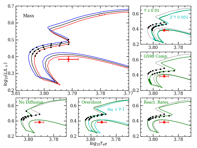
For comparison, we show exploratory MESA evolution models in Figure 14. For these experiments, the baseline inputs were a solar-calibrated Asplund et al. 2009 composition (, ) and mixing length parameter (), nuclear reaction rates from the JINA compilation, diffusion, and disabled core convective overshooting. Before proceeding, we note that convection or diffusion parameters produce minimal effects on the luminosity of the star as it moves away from the main sequence toward its temporary temperature minimum shortly before core hydrogen exhaustion. These factors play more of a role when discussing the rest of the turnoff in §4.3.
-
•
Measured mass: A stellar mass approximately lower than measured would allow the redward evolution of the model star to pass through the middle of the HR diagram error bars. This would be a error according to our calculations, however, and seems unlikely. We note that a star of still produces a significant convective core at the end of its main sequence evolution in the MESA models.
-
•
Measured luminosity: If there is a systematic error in our decomposition of the binary’s light or in the distance of the system, it could account for some of the luminosity discrepancy. If the distance is underestimated (due to an overestimate in the parallax), the luminosity would be larger. The Gaia parallax correction would be a suspect because it is acting in this direction. The corrections being discussed (§3.2) would produce a maximum effect of 0.04 dex in , which is not enough to explain the full discrepancy, and even so, smaller distances become more inconsistent with CMD-based distance measures. As for the bolometric flux, we note that the star-based decomposition of the SED (instead of the main sequence fit) leads to a lower , and so would exacerbate the discrepancy if true.
-
•
Nuclear reaction rates: CNO cycle rates in a stellar evolution code affect the strength of the energy generation. Larger rates lead to an earlier initiation of the convective core and lower luminosity for the star during its redward evolution. The CNO cycle bottleneck reaction 14N(p,)15O is the most important to consider. The reaction rate was revised downward by nearly 50% at stellar energies as a consequence of a reduced contribution of capture to the ground state of 15O, making capture to the 6.792 MeV excited state the dominant channel. Summaries of relevant experimental measurements can be found in Adelberger et al. (2011) and Wagner et al. (2018). The NACRE reaction rate tabulation (Angulo et al., 1999) uses the older, higher astrophysical factor, while recent tabulations (Xu et al., 2013; Cyburt et al., 2010) use values consistent with the recent experimental results (Formicola et al., 2004; Imbriani et al., 2005). While there appears to be convergence on experimental details of the 14N(p,)15O reaction, the extrapolation of the factor to stellar energies now contributes the most to the uncertainty at the level of about 8% (Wagner et al., 2018). Although significant for other purposes (such as using solar neutrinos to address solar composition uncertainties), this level of uncertainty is too small to account for the luminosity discrepancy unless there is an unknown and more substantial systematic error in the model reaction rate.
The bottleneck reaction in CNO cycle II is 17ON, and this rate has recently been revised upward by a factor of 2 at stellar energies by Bruno et al. (2016). This affects the flow of 16O into the main CNO cycle, and so has a small effect on the luminosity. But again, within the likely uncertainties, reaction rates also fall far short of explaining the size of the luminosity discrepancy.
-
•
CNO and heavy element abundances: CNO element abundances affect the CNO cycle energy generation through their role as catalysts, and larger abundances allow the convective core to be established earlier in the main sequence evolution and at lower luminosity. As an illustration in the middle right panel of Figure 14, the use of a GS98 solar abundance mix moves the redward evolution to lower luminosity because that mix has a larger proportion of CNO elements and because solar calibration with this composition leads to a larger metallicity. However, even a nearly 25% change in the CNO elements is not enough to explain the luminosity discrepancy for WOCS 11028 A. As seen in the upper right panel of Figure 14, increased metal content also results in a reduced luminosity during the redward evolution. As discussed in section 4.1, evidence from recent spectroscopic studies suggests that subgiants (which should have deep enough outer convective zones to erase diffusion effects that occurred on the main sequence) have higher surface metal abundances than turnoff stars.
Reasonable changes to the bulk heavy element abundance can bring the models into agreement with the measured luminosity and temperature of WOCS 11028 A at its measured mass. However, if we assume that composition changes are responsible, then this affects the agreement of other well-measured stars with the models. In particular, the models become too low in luminosity to match WOCS 11028 B.
Our conclusion is that a larger bulk heavy element abundance for M67 stars (previously masked by diffusion effects) is the most significant effect on the agreement between models and the characteristics of WOCS 11028 A that we can identify. Figure 19 compares the characteristics of WOCS 11028 A with MESA models for and . In the plot, the faint cluster turnoff occurs at the age where the three tracks cross, indicating a constant temperature in the mass range shown. With the larger bulk metal content, the radius, effective temperature, and luminosity of the star are approximately in agreement with models for ages roughly between 3.5 and 4.0 Gyr. Further adjustment of would throw either the model or out of agreement with the observations, although the radius is less sensitive to metal content.
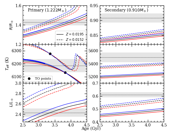
If the same large metal abundance is applied to models of WOCS 11028 B, they are pushed farther from agreement with the observations, however. The radius in particular should not be sensitive to the metal content, but the models are significantly lower than the observations for reasonable ages. As seen in Figure 16, the measurements of WOCS 11028 B agree with those for other well-measured eclipsing binary star components. As a result, we think that there are still unidentified systematic errors that are playing a role.
4.3 The Turnoff of M67 and Convective Cores
With the new data on the massive star in the WOCS 11028 binary, there is an opportunity to re-examine the cluster turnoff and the constraints it places on the age and stellar physics. We can make a more precise estimate of star masses at the turnoff than has been possible before by employing models that are capable of reproducing the characteristics of WOCS 11028 A, reducing the importance of systematic errors by making a relative comparison. The observed properties of the CMD gap and the upper turnoff are strongly influenced by the extent of the convective core, which in turn affects the amount of accessible fuel and the main sequence lifetimes.
A major uncertainty about convective core extent is overshooting of the convective boundary. The stars at M67’s turnoff are uniquely interesting because they are close to the minimum mass for having convective cores, and the amount of overshooting could play an outsized role in stars with small cores. Some studies of eclipsing binaries in the mass range (Claret & Torres, 2017, 2018) indicate that convective overshooting is consistent with zero at the mass of WOCS 11028 A, but rapidly increasing to a plateau for masses greater than about . On the other hand, the models of Higl & Weiss (2017) also show little or no need for overshooting in binaries with main sequence stars having masses near , but some weak evidence for overshooting in BG Ind, having a somewhat more massive () and more evolved primary star. Constantino & Baraffe (2018) found little evidence for a mass-dependent overshooting for masses between 1.2 and . A major problem with the binary star samples in most of these studies is that overshooting reveals itself most clearly very close to core hydrogen exhaustion, and unless stars are in a very specific evolutionary phase, their conventional stellar properties (like , , and ) will not be sensitive to the overshooting. This disagreement in the literature reinforces the value of using the information contained in M67, with its larger sample of stars and mass inferences from the WOCS 11028 binary.
More recently, a number of asteroseismic studies have also attempted to constrain convective core overshooting with low-degree p modes. Studies like Viani & Basu (2020) find positive trends in overshooting amount with mass, while others like Angelou et al. (2020) find overshooting amounts that are consistent with what is found from binary and cluster calibrations but without evidence of a clear mass dependence. These issues highlight that there are systematics and degeneracies in the fitting of parameters in asteroseismic studies, and that they have not fully clarified the overshoot issue. Asteroseismic masses have significantly lower precisions than binary system masses as well. All of these factors call out for additional precise constraints on the overshooting in this mass range.
Overshooting did not play a significant role in our interpretation of the WOCS 11028 binary because the primary star is well before core hydrogen exhaustion, but it does more strongly affect the CMD positions of stars around the turnoff gap and beginning of the subgiant branch. Models indicate that a star like WOCS 11028 A reaches a maximum in surface temperature when the convective core starts expanding as the core temperature increases and the CNO cycle becomes more dominant. After the star passes its surface temperature maximum, models show that the convective core is maintained and the star evolves mostly in until shortly before core hydrogen exhaustion. At that time the convective core rapidly shrinks and disappears, and the star executes a quick movement to higher temperatures and luminosities in the HR Diagram. There is still a residue of hydrogen in the core and a steep gradient in hydrogen abundance outside that, so the evolution of the star slows down again in the early subgiant branch. Overall, this evolution track is a hybrid, with the early core hydrogen burning evolution similar to low-mass stars, and the late evolution similar to more massive stars.
The extent and lifetime of the convective core in stars slightly more massive than WOCS 11028 A is imprinted on the shape of the turnoff in the CMD and in the number of stars present. The noticeable gap seen at in M67 is a demonstration of the rapid evolution that results from the disappearance of the convective core shortly before central hydrogen exhaustion. Similarly, the fairly large density of stars present just brighter than the gap shows that gas with large hydrogen abundance is residing just outside the exhausted center of the star, and the burning of this hydrogen allows the evolution to slow down again.
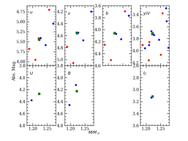
To define the shape of the turnoff, we derived bolometric fluxes and surface temperatures from SED fits for probable single stars at critical points in the CMD. We identified WOCS 7006 / Sanders 1003 as a likely single cluster member at the bright end of the gap based on CMD position and lack of radial velocity variation (Geller et al., 2015), and WOCS 8011 / Sanders 1219 as a likely single member at the faint end. We also examined WOCS 3003 / Sanders 1034 as a representative of the end of the most heavily populated part of the early subgiant branch. The stars are shown in CMDs in Figure 3, and their derived properties are given in Table 3.
| WOCS 3003 | WOCS 7006 | WOCS 8011 | WOCS 11028A | WOCS 11028B | |
|---|---|---|---|---|---|
| ( erg cm-2 s-1) | |||||
| () | |||||
| 13.568 | 15.167 | ||||
| 0.372 | 0.486 | ||||
| 0.394 | 0.321 | ||||
| H | |||||
| (K) | 6225 | 6150 | 6225 | ||
| (IRFM) (K) | 6010 | 6170 | 6080 | 6185 | 5500 |
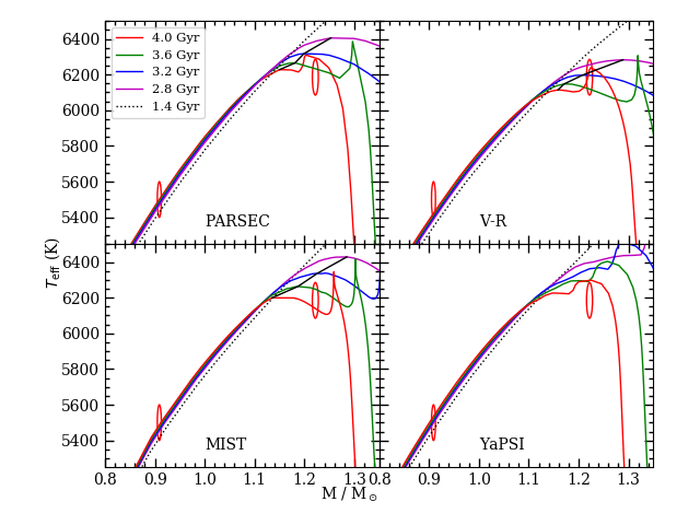
As was shown in Figure 14, several model physics parameters play a role in setting the shape of the turnoff and subgiant branch, and most affect core convection. As a result, there is some degeneracy in the parameters that can be used to model the turnoff. For our purposes here, we will focus on convective core overshooting. Overshooting has the most substantial effects on evolution tracks shortly before the time of core hydrogen exhaustion. Core hydrogen exhaustion is delayed by overshooting, which allows the redward evolution to extend to lower temperature, giving isochrones a deeper redward kink (see bottom middle panel of Figure 14). In addition, the morphology of the upper turnoff changes in response to overshooting, with increasing amounts resulting in a more horizontal early subgiant branch. (See Figure 13, and compare the BaSTI-IAC isochrones with and without overshooting, or younger PARSEC isochrones to older ones that have less overshoot.) Both the morphology of the upper turnoff and the luminosity and temperature positions of the stars measured near the gap in M67 are indicative of weaker convective overshooting than is used in the MIST isochrones. This is a means of calibrating overshoot for stars with masses around the gap (approximately , based on models that match WOCS 11028 A). The exact amount depends somewhat on other physics, like diffusion rates, CNO cycle reaction rates, and CNO element abundances.
It has long been known that the turnoff of M67 is not well matched by isochrones (VandenBerg et al., 2007; Magic et al., 2010). Currently published theoretical isochrones should not be used to calibrate the overshooting or read an age because they do not reproduce the characteristics of WOCS 11028 A (see Section 4.2.3), and would therefore have clear systematic errors. There are unfortunately several composition and physics factors that can affect the size (and even the presence) of a convective core in models, and relatively small changes in the extent of this core can strongly affect the amount of hydrogen fuel the core gets, and therefore, the length of the star’s life. But by using models that are at least able to match WOCS 11028 A, we should be able to reduce the size of the errors.
Figure 20 shows isochrones from MESA models having and , with convective core overshooting set to half the default value, or . Larger amounts of overshooting move the gap to lower temperatures, and appear to be ruled out. With this set of input parameters, we are able to approximately reproduce the HR diagram positions of the three stars (described above) that reside at identifiable points in the cluster CMD using an age around 3.75-4 Gyr. In addition, Stello et al. (2016) found an average giant star mass of in their asteroseismic analysis of M67 giant stars using K2 data. This measurement is also consistent with an age near 4 Gyr for the MESA models used in Figure 20. The agreement with all of these observations implies that the models are approximately reproducing the hydrogen abundance profile in the stars at core exhaustion.
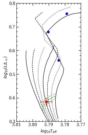
5 Conclusions
We present high-precision measurements of the masses, radii, and photometry for stars in the bright detached eclipsing binary system WOCS 11028 in the cluster M67. This cluster is commonly used as a testbed for stellar evolution models of solar metallicity, and the addition of new observables for stars in the cluster will further test the fidelity of the physics we use to model them.
Despite orbits that only produce one eclipse per cycle, we have shown that high-precision masses for the stars in WOCS 11028 are possible. We have used a decomposition of the SED of the binary to constrain the temperatures, radii, and luminosities of the stars as well. The brighter star in the binary sits precisely at the fainter turnoff point for the cluster, where stars with convective cores are accelerating toward the red in the later stages of core hydrogen burning. The known mass of a star at an identifiable evolutionary point constrains the age of the cluster, although uncertainties in model physics reduce the precision that is attainable.
Systematic errors in the model physics remain a difficult problem for stars at the turnoff of M67. Recent spectroscopic studies seem to make a strong case for the inclusion of diffusion in models, and a larger bulk metallicity for cluster stars can explain the characteristics of WOCS 11028 A. However, the cost of this is a disgreement between fainter stars (solar analogs and less massive stars) and models. We are forced to the conclusion that there appears to be an unidentified systematic error that affects the luminosities of stars between (and possibly including) 1 and . Our examination of physics uncertainties like nuclear reaction rates, convection, and chemical composition has not revealed an obvious culprit. With the assumption of a larger bulk metallicity, age indicators are somewhat consistent in returning ages between about 3.5 and 4 Gyr. Future adjustments to model physics will hopefully provide greater agreement between the measures.
With a star of known mass at the lower cluster turnoff, we can more reliably calibrate models of stars at core hydrogen exhaustion, which are sensitive to the size of the convective core. The morphology of M67’s turnoff implies that convective overshooting in turnoff mass stars is present, but to an extent that is smaller than used in standard isochrones. After identifying composition and physics parameters that allow us to match the characteristics of WOCS 11028 A, we can estimate the mass of stars at the turnoff of M67. We find that stars near the gap and upper turnoff should have masses of . With these same model parameters, we can approximately match the average asteroseismic giant mass of measured by Stello et al. (2016) at an age near 4 Gyr. More precise comparisons between observed masses and theory will require a better understanding of the core convection physics because this critically affects the timing of a star’s divergence from the main sequence. Precise and direct measurements of masses in the eclipsing system HV Cnc could improve the comparison as well because the brightest star resides at the upper turnoff. The difficulties in completing such a study are the faintness of the companion and the contaminating effects of an unresolved third star (Sandquist & Shetrone, 2003). However, this is one of the few ways of further identifying and eliminating the systematic errors in our modeling of these stars and our determination of their ages.
References
- Adelberger et al. (2011) Adelberger, E. G., García, A., Robertson, R. G. H., et al. 2011, Reviews of Modern Physics, 83, 195
- Andersen et al. (1989) Andersen, J., Clausen, J. V., & Magain, P. 1989, A&A, 211, 346
- Andersen (1991) Andersen, J. 1991, A&A Rev., 3, 91
- Angelou et al. (2020) Angelou, G. C., Bellinger, E. P., Hekker, S., et al. 2020, MNRAS, 493, 4987.
- Angulo et al. (1999) Angulo, C., Arnould, M., Rayet, M., et al. 1999, Nuclear Physics A, 656, 3
- Angus et al. (2015) Angus, R., Aigrain, S., Foreman-Mackey, D., et al. 2015, MNRAS, 450, 1787
- Asplund et al. (2009) Asplund, M., Grevesse, N., Sauval, A. J., & Scott, P. 2009, ARA&A, 47, 481
- Balaguer-Núñez et al. (2007) Balaguer-Núñez, L., Galadí-Enríquez, D., & Jordi, C. 2007, A&A, 470, 585
- Bertelli Motta et al. (2018) Bertelli Motta, C., Pasquali, A., Richer, J., et al. 2018, MNRAS, 478, 425
- Bessell et al. (1998) Bessell, M. S., Castelli, F., & Plez, B. 1998, A&A, 333, 231
- Blackwell & Shallis (1977) Blackwell, D. E., & Shallis, M. J. 1977, MNRAS, 180, 177
- Bressan et al. (2012) Bressan, A., Marigo, P., Girardi, L., et al. 2012, MNRAS, 427, 127
- Brewer et al. (2016) Brewer, L. N., Sandquist, E. L., Mathieu, R. D., et al. 2016, AJ, 151, 66
- Bruno et al. (2016) Bruno, C. G., Scott, D. A., Aliotta, M., et al. 2016, Phys. Rev. Lett., 117, 142502
- Cardelli et al. (1989) Cardelli, J. A., Clayton, G. C., & Mathis, J. S. 1989, ApJ, 345, 245
- Carrera et al. (2019) Carrera, R., Pasquato, M., Vallenari, A., et al. 2019, A&A, 627, A119
- Casagrande et al. (2010) Casagrande, L., Ramírez, I., Meléndez, J., et al. 2010, A&A, 512, A54
- Casagrande & VandenBerg (2014) Casagrande, L., & VandenBerg, D. A. 2014, MNRAS, 444, 392
- Castelli & Kurucz (2004) Castelli, F., & Kurucz, R. L. 2004, arXiv:astro-ph/0405087
- Choi et al. (2016) Choi, J., Dotter, A., Conroy, C., et al. 2016, ApJ, 823, 102
- Claret & Torres (2017) Claret, A., & Torres, G. 2017, ApJ, 849, 18
- Claret & Torres (2018) Claret, A., & Torres, G. 2018, ApJ, 859, 100
- Clausen et al. (2008) Clausen, J. V., Torres, G., Bruntt, H., et al. 2008, A&A, 487, 1095
- Clausen et al. (2010) Clausen, J. V., Frandsen, S., Bruntt, H., et al. 2010, A&A, 516, A42
- Coelho et al. (2005) Coelho, P., Barbuy, B., Meléndez, J., Schiavon, R. P., & Castilho, B. V. 2005, A&A, 443, 735
- Coelho (2014) Coelho, P. R. T. 2014, MNRAS, 440, 1027
- Cohen et al. (2003) Cohen, M., Wheaton, W. A., & Megeath, S. T. 2003, AJ, 126, 1090
- Constantino & Baraffe (2018) Constantino, T. & Baraffe, I. 2018, A&A, 618, A177.
- Cosentino et al. (2012) Cosentino, R., Lovis, C., Pepe, F., et al. 2012, Proc. SPIE, 8446, 84461V
- Cyburt et al. (2010) Cyburt, R. H., Amthor, A. M., Ferguson, R., et al. 2010, ApJS, 189, 240
- Dotter (2016) Dotter, A. 2016, ApJS, 222, 8
- Evans et al. (2018) Evans, D. W., Riello, M., De Angeli, F., et al. 2018, A&A, 616, A4
- Fan et al. (1996) Fan, X., Burstein, D., Chen, J.-S., et al. 1996, AJ, 112, 628
- Finkbeiner et al. (2016) Finkbeiner, D. P., Schlafly, E. F., Schlegel, D. J., et al. 2016, ApJ, 822, 66
- Foreman-Mackey et al. (2013) Foreman-Mackey, D., Hogg, D. W., Lang, D., & Goodman, J. 2013, PASP, 125, 306
- Formicola et al. (2004) Formicola, A., Imbriani, G., Costantini, H., et al. 2004, Physics Letters B, 591, 61
- Gaia Collaboration et al. (2018a) Gaia Collaboration, Brown, A. G. A., Vallenari, A., et al. 2018, A&A, 616, A1
- Gaia Collaboration et al. (2018b) Gaia Collaboration, Babusiaux, C., van Leeuwen, F., et al. 2018, A&A, 616, A10
- Gao et al. (2018) Gao, X., Lind, K., Amarsi, A. M., et al. 2018, MNRAS, 481, 2666
- Geller et al. (2015) Geller, A. M., Latham, D. W., & Mathieu, R. D. 2015, AJ, 150, 97
- Girard et al. (1989) Girard, T. M., Grundy, W. M., Lopez, C. E., & van Altena, W. F. 1989, AJ, 98, 227
- Gökay et al. (2020) Gökay, G., Özdemir, S., & Gürol, B. 2020, New A, 75, 101302
- González & Levato (2006) González, J. F., & Levato, H. 2006, A&A, 448, 283
- Graczyk et al. (2016) Graczyk, D., Smolec, R., Pavlovski, K., et al. 2016, A&A, 594, A92
- Gray (1998) Gray, R. O. 1998, AJ, 116, 482
- Grevesse & Sauval (1998) Grevesse, N., & Sauval, A. J. 1998, Space Sci. Rev., 85, 161
- Hełminiak et al. (2009) Hełminiak, K. G., Konacki, M., Ratajczak, M., et al. 2009, MNRAS, 400, 969
- Hełminiak et al. (2019) Hełminiak, K. G., Konacki, M., Maehara, H., et al. 2019, MNRAS, 484, 451
- Henden et al. (2015) Henden, A. A., Levine, S., Terrell, D., et al. 2015, American Astronomical Society Meeting Abstracts #225 225, 336.16
- Hidalgo et al. (2018) Hidalgo, S. L., Pietrinferni, A., Cassisi, S., et al. 2018, ApJ, 856, 125
- Higl & Weiss (2017) Higl, J., & Weiss, A. 2017, A&A, 608, A62
- Holtzman et al. (2015) Holtzman, J. A., Shetrone, M., Johnson, J. A., et al. 2015, AJ, 150, 148
- Hut (1981) Hut, P. 1981, A&A, 99, 126
- Imbriani et al. (2005) Imbriani, G., Costantini, H., Formicola, A., et al. 2005, European Physical Journal A, 25, 455
- Kaiser et al. (2010) Kaiser, N., Burgett, W., Chambers, K., et al. 2010, Proc. SPIE, 7733, 77330E
- Kipping (2013) Kipping, D. M. 2013, MNRAS, 435, 2152
- Krone-Martins et al. (2010) Krone-Martins, A., Soubiran, C., Ducourant, C., Teixeira, R., & Le Campion, J. F. 2010, A&A, 516, A3
- Kwee & van Woerden (1956) Kwee, K. K., & van Woerden, H. 1956, Bull. Astron. Inst. Netherlands, 12, 327
- Lacy & Fekel (2014) Lacy, C. H. S., & Fekel, F. C. 2014, AJ, 148, 71
- Lacy et al. (2014) Lacy, C. H. S., Torres, G., Fekel, F. C., et al. 2014, AJ, 147, 148
- Latham (1985) Latham, D. W. 1985, Stellar Radial Velocities, 88, 21
- Latham (1992) Latham, D. W. 1992, IAU Colloq. 135: Complementary Approaches to Double and Multiple Star Research, 32, 110
- Laugalys et al. (2004) Laugalys, V., Kazlauskas, A., Boyle, R. P., et al. 2004, Baltic Astronomy, 13, 1
- Lindegren et al. (2018) Lindegren, L., Hernández, J., Bombrun, A., et al. 2018, A&A, 616, A2
- Liu et al. (2019) Liu, F., Asplund, M., Yong, D., et al. 2019, A&A, 627, A117
- Luger et al. (2018) Luger, R., Kruse, E., Foreman-Mackey, D., et al. 2018, AJ, 156, 99
- Magic et al. (2010) Magic, Z., Serenelli, A., Weiss, A., & Chaboyer, B. 2010, ApJ, 718, 1378
- Mann & von Braun (2015) Mann, A. W., & von Braun, K. 2015, PASP, 127, 102
- Marigo et al. (2017) Marigo, P., Girardi, L., Bressan, A., et al. 2017, ApJ, 835, 77
- Marta et al. (2008) Marta, M., Formicola, A., Gyürky, G., et al. 2008, Phys. Rev. C, 78, 022802
- Martin et al. (2005) Martin, D. C., Fanson, J., Schiminovich, D., et al. 2005, ApJ, 619, L1
- Mathieu et al. (2016) Mathieu, R. D., Vanderburg, A., & K2 M67 Team 2016, American Astronomical Society Meeting Abstracts, 228, 117.04
- Montgomery et al. (1993) Montgomery, K. A., Marschall, L. A., & Janes, K. A. 1993, AJ, 106, 181
- Morrissey et al. (2007) Morrissey, P., Conrow, T., Barlow, T. A., et al. 2007, ApJS, 173, 682
- Nardiello et al. (2016a) Nardiello, D., Libralato, M., Bedin, L. R., et al. 2016, MNRAS, 455, 2337
- Nardiello et al. (2016b) Nardiello, D., Libralato, M., Bedin, L. R., et al. 2016, MNRAS, 463, 1831
- Nissen et al. (1987) Nissen, P. E., Twarog, B. A., & Crawford, D. L. 1987, AJ, 93, 634
- Önehag et al. (2014) Önehag, A., Gustafsson, B., & Korn, A. 2014, A&A, 562, A102
- Oke & Gunn (1983) Oke, J. B., & Gunn, J. E. 1983, ApJ, 266, 713
- Orosz & Hauschildt (2000) Orosz, J. A., & Hauschildt, P. H. 2000, A&A, 364, 265
- Ochsenbein et al. (2000) Ochsenbein, F., Bauer, P., & Marcout, J. 2000, A&AS, 143, 23
- Pace et al. (2012) Pace, G., Castro, M., Meléndez, J., Théado, S., & do Nascimento, J.-D., Jr. 2012, A&A, 541, A150
- Page et al. (2014) Page, M. J., Yershov, V., Breeveld, A., et al. 2014, Proceedings of Swift: 10 Years of Discovery (SWIFT 10), held 2-5 December 2014 at La Sapienza University, Rome, Italy. Online at http://pos.sissa.it/cgi-bin/reader/conf.cgi?confid=233, id.37, 37
- Pasquini et al. (2008) Pasquini, L., Biazzo, K., Bonifacio, P., Randich, S., & Bedin, L. R. 2008, A&A, 489, 677
- Paxton et al. (2011) Paxton, B., Bildsten, L., Dotter, A., et al. 2011, ApJS, 192, 3
- Paxton et al. (2013) Paxton, B., Cantiello, M., Arras, P., et al. 2013, ApJS, 208, 4
- Paxton et al. (2015) Paxton, B., Marchant, P., Schwab, J., et al. 2015, ApJS, 220, 15
- Paxton et al. (2018) Paxton, B., Schwab, J., Bauer, E. B., et al. 2018, ApJS, 234, 34
- Paxton et al. (2019) Paxton, B., Smolec, R., Schwab, J., et al. 2019, ApJS, 243, 10
- Pickles (1998) Pickles, A. J. 1998, PASP, 110, 863
- Poole et al. (2008) Poole, T. S., Breeveld, A. A., Page, M. J., et al. 2008, MNRAS, 383, 627
- Popper et al. (1986) Popper, D. M., Lacy, C. H., Frueh, M. L., et al. 1986, AJ, 91, 383
- Rucinski (2002) Rucinski, S. M., 2002, AJ, 124, 1746
- Sanders (1977) Sanders, W. L. 1977, A&AS, 27, 89
- Sandquist & Shetrone (2003) Sandquist, E. L., & Shetrone, M. D. 2003, AJ, 126, 2954
- Sandquist et al. (2018) Sandquist, E. L., Mathieu, R. D., Quinn, S. N., et al. 2018, AJ, 155, 152
- Sandquist (2004) Sandquist, E. L. 2004, MNRAS, 347, 101
- Sarajedini et al. (2009) Sarajedini, A., Dotter, A., & Kirkpatrick, A. 2009, ApJ, 698, 1872
- Schönrich et al. (2019) Schönrich, R., McMillan, P., & Eyer, L. 2019, MNRAS, 487, 3568
- Schlafly et al. (2012) Schlafly, E. F., Finkbeiner, D. P., Jurić, M., et al. 2012, ApJ, 756, 158
- Short et al. (2018) Short, D. R., Orosz, J. A., Windmiller, G., et al. 2018, AJ, 156, 297
- Skrutskie et al. (2006) Skrutskie, M. F. et al. 2006, AJ, 131, 1163
- Southworth (2015) Southworth, J. 2015, Living Together: Planets, Host Stars and Binaries, 496, 164
- Souto et al. (2019) Souto, D., Allende Prieto, C., Cunha, K., et al. 2019, ApJ, 874, 97
- Spada et al. (2017) Spada, F., Demarque, P., Kim, Y.-C., Boyajian, T. S., & Brewer, J. M. 2017, ApJ, 838, 161
- Stassun & Torres (2018) Stassun, K. G. & Torres, G. 2018, ApJ, 862, 61
- Stello et al. (2016) Stello, D., Vanderburg, A., Casagrande, L., et al. 2016, ApJ, 832, 133
- Taylor (2007) Taylor, B. J. 2007, AJ, 133, 370
- Ter Braak (2006) Ter Braak, C. J. F. 2006, Stat. Comput., 16, 239
- Tody (1986) Tody, D. 1986, Proc. SPIE, 627, 733
- Tody (1993) Tody, D. 1993, Astronomical Data Analysis Software and Systems II, 52, 173
- Torres et al. (2010) Torres, G., Andersen, J., & Giménez, A. 2010, A&A Rev., 18, 67
- VandenBerg et al. (2006) VandenBerg, D. A., Bergbusch, P. A., & Dowler, P. D. 2006, ApJS, 162, 375
- VandenBerg et al. (2007) VandenBerg, D. A., Gustafsson, B., Edvardsson, B., Eriksson, K., & Ferguson, J. 2007, ApJ, 666, L105
- VandenBerg & Stetson (2004) VandenBerg, D. A., & Stetson, P. B. 2004, PASP, 116, 997
- Vanderburg & Johnson (2014) Vanderburg, A., & Johnson, J. A. 2014, PASP, 126, 948
- Vanderburg et al. (2016) Vanderburg, A., Latham, D. W., Buchhave, L. A., et al. 2016, ApJS, 222, 14
- Viani & Basu (2020) Viani, L. S. & Basu, S. 2020, arXiv:2009.09344
- Vos et al. (2012) Vos, J., Clausen, J. V., Jørgensen, U. G., et al. 2012, A&A, 540, A64
- Wagner et al. (2018) Wagner, L., Akhmadaliev, S., Anders, M., et al. 2018, Phys. Rev. C, 97, 015801
- Wright et al. (2010) Wright, E. L., Eisenhardt, P. R. M., Mainzer, A. K., et al. 2010, AJ, 140, 1868
- Xu et al. (2013) Xu, Y., Takahashi, K., Goriely, S., et al. 2013, Nucl. Phys. A, 918, 61
- Yadav et al. (2008) Yadav, R. K. S., Bedin, L. R., Piotto, G., et al. 2008, A&A, 484, 609
- York et al. (2000) York, D. G., Adelman, J., Anderson, J. E., Jr., et al. 2000, AJ, 120, 1579
- Zamora et al. (2015) Zamora, O., García-Hernández, D. A., Allende Prieto, C., et al. 2015, AJ, 149, 181
- Zhao et al. (1993) Zhao, J. L., Tian, K. P., Pan, R. S., He, Y. P., & Shi, H. M. 1993, A&AS, 100, 243
- Zhou et al. (2003) Zhou, X., Jiang, Z., Ma, J., et al. 2003, A&A, 397, 361
- Zinn et al. (2019) Zinn, J. C., Pinsonneault, M. H., Huber, D., et al. 2019, ApJ, 878, 136
| Bright Component A | Faint Component B | Ratios | ||||||||||
|---|---|---|---|---|---|---|---|---|---|---|---|---|
| WOCS 11028 | WOCS 6018 | MS Fit | WOCS 10027 | MS Fit | Stars | MS Fit | ||||||
| Filter | (Å) | Ref. | ||||||||||
| 2030 | 16.715 | 0.058 | 16.898 | 0.040 | 16.886 | 19.389 | 0.100 | |||||
| 2231 | 16.655 | 0.072 | 16.757 | 0.050 | ||||||||
| NUV | 2315.7 | 18.164 | 0.006 | 18.230 | 0.008 | 18.221 | 21.047 | 0.049 | 21.277 | 0.075 | 0.060 | |
| 2634 | 15.228 | 0.030 | 15.390 | 0.021 | 15.382 | 17.753 | 0.113 | |||||
| 3450 | 15.953 | 0.018 | 18.030 | 0.145 | 1 | |||||||
| 3520 | 15.283 | 0.004 | 15.476 | 0.004 | 15.386 | 17.183 | 0.016 | 17.470 | 0.208 | 0.147 | 2 | |
| 3551 | 14.851 | 0.009 | 15.025 | 0.014 | 14.993 | 16.825 | 0.029 | 17.096 | 0.191 | 0.144 | ||
| 3663 | 14.144 | 14.202 | 15.962 | 16.308 | 0.187 | 0.144 | 3 | |||||
| 3740 | 15.475 | 0.013 | 15.449 | 17.590 | 0.139 | 1 | ||||||
| BATC2 () | 3890 | 14.39 | 0.01 | 14.59 | 0.02 | 14.539 | 16.45 | 0.05 | 16.695 | 0.180 | 0.137 | 4 |
| 4054 | 14.882 | 0.011 | 14.854 | 16.825 | 0.163 | 1 | ||||||
| 4100 | 14.308 | 0.003 | 14.522 | 0.002 | 14.466 | 16.155 | 0.014 | 16.401 | 0.222 | 0.168 | 2 | |
| 4361 | 14.125 | 15.739 | 0.006 | 15.930 | 0.190 | 5 | ||||||
| 4361 | 14.149 | 14.149 | 15.758 | 0.015 | 15.960 | 0.227 | 0.189 | 3 | ||||
| 4361 | 13.971 | 0.068 | 14.164 | 0.031 | 14.118 | 15.786 | 0.096 | 15.955 | 0.224 | 0.184 | 6 | |
| 4361 | 13.952 | 14.183 | 14.151 | 15.627 | 15.960 | 0.264 | 0.189 | 7 | ||||
| 4361 | 13.881 | 0.013 | 14.123 | 15.675 | 0.004 | 15.912 | 0.193 | 8 | ||||
| BATC4 () | 4532 | 13.67 | 0.01 | 13.92 | 0.01 | 13.879 | 15.41 | 0.01 | 15.620 | 0.254 | 0.201 | 4 |
| 4665 | 14.148 | 0.008 | 14.117 | 15.827 | 0.207 | 1 | ||||||
| 4640 | 13.759 | 0.386 | 13.979 | 0.307 | 13.807 | 15.360 | 0.176 | 15.481 | 0.280 | 0.214 | 6 | |
| 4686 | 13.592 | 0.001 | 13.825 | 0.008 | 13.816 | 15.292 | 0.010 | 15.491 | 0.259 | 0.214 | ||
| 4688 | 13.720 | 0.002 | 13.979 | 0.002 | 13.940 | 15.454 | 0.011 | 15.653 | 0.257 | 0.207 | 2 | |
| 4810 | 13.560 | 0.001 | 13.784 | 0.001 | 13.743 | 15.224 | 0.003 | 15.425 | 0.266 | 0.212 | ||
| BATC5 () | 4916 | 13.53 | 0.01 | 13.78 | 0.01 | 13.710 | 15.17 | 0.01 | 15.375 | 0.278 | 0.216 | 4 |
| 5051.5 | 13.5113 | 0.0013 | 13.7714 | 0.0011 | 13.7289 | 15.1898 | 0.0016 | 15.3801 | 0.271 | 0.219 | ||
| 5162 | 13.815 | 0.008 | 13.777 | 15.451 | 0.214 | 1 | ||||||
| BATC6 () | 5258 | 13.38 | 0.01 | 13.65 | 0.01 | 13.585 | 15.03 | 0.02 | 15.225 | 0.281 | 0.221 | 4 |
| 5442 | 13.622 | 0.006 | 13.582 | 15.182 | 0.229 | 1 | ||||||
| 5448 | 13.337 | 0.001 | 13.597 | 0.001 | 13.564 | 14.953 | 0.002 | 15.152 | 0.287 | 0.232 | 5 | |
| 5448 | 13.598 | 13.597 | 15.010 | 0.010 | 15.183 | 0.275 | 0.227 | 3 | ||||
| 5448 | 13.366 | 0.042 | 13.619 | 0.011 | 13.566 | 14.977 | 0.047 | 15.158 | 0.286 | 0.231 | 6 | |
| 5448 | 13.391 | 13.675 | 13.597 | 15.174 | 0.234 | 7 | ||||||
| 5448 | 13.246 | 0.004 | 13.539 | 14.924 | 0.007 | 15.123 | 0.232 | 8 | ||||
| 5480 | 13.349 | 0.003 | 13.616 | 0.003 | 13.568 | 14.974 | 0.008 | 15.167 | 0.286 | 0.229 | 2 | |
| BATC7 () | 5785 | 13.24 | 0.02 | 13.55 | 0.02 | 13.473 | 14.84 | 0.03 | 15.013 | 0.305 | 0.242 | 4 |
| BATC8 () | 6069 | 13.16 | 0.02 | 13.44 | 0.02 | 13.380 | 14.70 | 0.03 | 14.901 | 0.313 | 0.246 | 4 |
| 6122 | 13.194 | 0.019 | 13.491 | 0.019 | 13.440 | 14.737 | 0.041 | 14.952 | 0.317 | 0.248 | 6 | |
| 6166 | 13.166 | 0.001 | 13.487 | 0.017 | 13.410 | 14.769 | 0.010 | 14.911 | 0.307 | 0.251 | ||
| 6170 | 13.482 | 0.013 | 13.426 | 14.756 | 0.001 | 14.926 | 0.309 | 0.251 | ||||
| 6230.6 | 13.1974 | 0.0002 | 13.4816 | 0.0002 | 13.4363 | 14.8044 | 0.0003 | 14.9717 | 0.296 | 0.243 | ||
| 6534 | 13.112 | 0.008 | 13.062 | 14.546 | 0.255 | 1 | ||||||
| BATC9 () | 6646 | 13.13 | 0.02 | 13.44 | 0.01 | 13.394 | 14.66 | 0.03 | 14.859 | 0.325 | 0.259 | 4 |
| BATC10a () | 7055 | 13.08 | 0.01 | 13.39 | 0.01 | 13.327 | 14.66 | 0.03 | 14.786 | 0.334 | 0.261 | 4 |
| 7440 | 13.264 | 0.369 | 13.528 | 0.305 | 13.374 | 14.545 | 0.072 | 14.790 | 0.392 | 0.271 | 6 | |
| 7480 | 13.357 | 0.001 | 13.308 | 14.602 | 0.021 | 14.742 | 0.318 | 0.267 | ||||
| 7520 | 13.225 | 13.465 | 13.337 | 14.618 | 0.003 | 14.748 | 0.346 | 0.273 | ||||
| BATC10b () | 7545 | 13.06 | 0.01 | 13.37 | 0.01 | 13.308 | 14.53 | 0.04 | 14.740 | 0.344 | 0.267 | 4 |
| 7726.2 | 12.7237 | 0.0007 | 13.0354 | 0.0006 | 12.9865 | 14.2558 | 0.0014 | 14.4074 | 0.325 | 0.270 | ||
| 7980 | 12.655 | 0.001 | 12.957 | 0.002 | 12.919 | 14.132 | 0.002 | 14.325 | 0.339 | 0.274 | 5 | |
| 7980 | 12.920 | 12.888 | 14.176 | 14.325 | 0.314 | 0.266 | 3 | |||||
| 7900 | 12.981 | 0.008 | 12.934 | 14.355 | 0.270 | 1 | ||||||
| 7900 | 12.584 | 0.005 | 12.874 | 14.107 | 0.002 | 14.311 | 0.266 | 8 | ||||
| BATC11 () | 8020 | 13.04 | 0.01 | 13.35 | 0.01 | 13.283 | 14.48 | 0.02 | 14.697 | 0.353 | 0.272 | 4 |
| BATC12 () | 8483 | 13.01 | 0.01 | 13.34 | 0.01 | 13.289 | 14.49 | 0.01 | 14.679 | 0.347 | 0.278 | 4 |
| 8660 | 13.058 | 0.004 | 13.387 | 0.003 | 13.339 | 14.579 | 0.002 | 14.715 | 0.334 | 0.282 | ||
| 8932 | 13.010 | 0.016 | 13.350 | 0.011 | 13.291 | 14.602 | 0.021 | 14.661 | 0.344 | 0.283 | ||
| BATC13 () | 9180 | 12.97 | 0.01 | 13.30 | 0.01 | 13.246 | 14.41 | 0.01 | 14.610 | 0.360 | 0.285 | |
| 9620 | 13.037 | 0.005 | 13.366 | 0.007 | 13.318 | 14.527 | 0.010 | 14.667 | 0.343 | 0.289 | ||
| BATC14 () | 9736 | 12.99 | 0.01 | 13.31 | 0.01 | 13.281 | 14.43 | 0.01 | 14.630 | 0.360 | 0.289 | |
| 12350 | 12.177 | 0.018 | 12.546 | 0.022 | 12.492 | 13.609 | 0.036 | 13.767 | 0.376 | 0.309 | ||
| 16620 | 11.903 | 0.020 | 12.260 | 0.020 | 12.237 | 13.276 | 0.042 | 13.391 | 0.392 | 0.346 | ||
| 21590 | 11.829 | 0.020 | 12.239 | 0.023 | 12.177 | 13.205 | 0.024 | 13.311 | 0.411 | 0.352 | ||
| 33526 | 11.799 | 0.023 | 12.211 | 0.024 | 12.131 | 13.015 | 0.030 | 13.264 | 0.477 | 0.352 | ||
| 46028 | 11.839 | 0.021 | 12.250 | 0.415 | 12.165 | 13.095 | 13.311 | 0.459 | 0.348 | |||
| (K) | 6200 | 100 | 6200 | 5600 | 100 | 5500 | 0.88 | 0.89 | ||||
| ( erg / cm2 s) | 10.47 | 10.89 | 3.21 | 2.73 | 0.310 | 0.248 | ||||||
| () | 0.719 | 0.643 | ||||||||||
| Name | (mas) | Filter | Magnitude | Refs.aaReferences: 1: Clausen et al. (2008). 2: Clausen et al. (2010). 3: Lacy et al. (2014). 4: Lacy & Fekel (2014). 5: Vos et al. (2012). 6: Hełminiak et al. (2009); Andersen et al. (1989). 7: Hełminiak et al. (2019); Popper et al. (1986). 8: Graczyk et al. (2016). 9: Brewer et al. (2016). | ||
|---|---|---|---|---|---|---|
| AD Boo B | 0.034 | 1 | ||||
| BK Peg B | 0.061 | 2 | ||||
| AP And A | 0.058 | 11.845 | 3 | |||
| AP And B | 0.058 | 11.963 | 3 | |||
| VZ Hya A | 0.028 | 1 | ||||
| V501 Her A | 0.048 | 4 | ||||
| V501 Her B | 0.048 | 4 | ||||
| EF Aqr A | 0. | 5 | ||||
| WZ Oph A | 0.045 | 1 | ||||
| WZ Oph B | 0.045 | 1 | ||||
| UX Men A | 0.028 | 6 | ||||
| UX Men B | 0.028 | 6 | ||||
| FL Lyr A | 0.007 | 7 | ||||
| LL Aqr A | 0.018 | 8 | ||||
| WOCS 40007 A | 0.16 | 0.420bbDistance modulus from Brewer et al. (2016) translated back into an equivalent parallax. | 9 | |||