The jump filter in the discontinuous Galerkin method for hyperbolic conservation laws
Abstract
When simulating hyperbolic conservation laws with discontinuous solutions, high-order linear numerical schemes often produce undesirable spurious oscillations. In this paper, we propose a jump filter within the discontinuous Galerkin (DG) method to mitigate these oscillations. This filter operates locally based on jump information at cell interfaces, targeting high-order polynomial modes within each cell. Besides its localized nature, our proposed filter preserves key attributes of the DG method, including conservation, stability, and high-order accuracy. We also explore its compatibility with other damping techniques, and demonstrate its seamless integration into a hybrid limiter. In scenarios featuring strong shock waves, this hybrid approach, incorporating this jump filter as the low-order limiter, effectively suppresses numerical oscillations while exhibiting low numerical dissipation. Additionally, the proposed jump filter maintains the compactness of the DG scheme, which greatly aids in efficient parallel computing. Moreover, it boasts an impressively low computational cost, given that no characteristic decomposition is required and all computations are confined to physical space. Numerical experiments validate the effectiveness and performance of our proposed scheme, confirming its accuracy and shock-capturing capabilities.
Key words: hyperbolic conservation laws; discontinuous Galerkin method; viscosity; jump filter; shock capture; steady-state.
1 Introduction
Developing robust, accurate, and efficient high-order schemes for numerically solving hyperbolic nonlinear systems of conservation laws is crucial. Hyperbolic conservation laws are fundamental partial differential equations (PDEs) that bridge mathematics and mechanics, reflecting natural wave phenomena and finding wide applications in fluid dynamics, magnetohydrodynamics, multiphase flow, population dynamics, traffic flow, etc. Despite smooth initial and boundary conditions, nonlinear hyperbolic systems may exhibit flow-field discontinuities, such as shocks and contact discontinuities. The lack of robustness, especially concerning nonlinear instabilities, presents a significant challenge in applying high-order numerical schemes to technical problems. High-order approximations of these discontinuities may result in unbounded oscillations, leading to solver divergence. Hence, the development of shock-capturing techniques has received considerable attention in recent years to tackle this issue.
There has been an abundance of work on the extension of classical shock-capturing methodologies to higher-order methods over the past three decades. Some popular higher-order shock-capturing methods include essentially non-oscillatory (ENO) schemes [24], weighted ENO (WENO) methods [48, 39], subcell finite volume shock-capturing methods [68, 56], and Runge-Kutta discontinuous Galerkin (RKDG) methods, just to name a few. Unlike WENO-type methods, DG methods do not require any reconstruction procedure since the numerical solution in each cell is already a polynomial of suitable degree. Since complete discontinuous basis functions are used, DG methods also have some advantages different from classical finite element methods, such as the allowance of arbitrary unstructured meshes with hanging nodes, and easy - adaptivity. It’s worth noting that DG methods exhibit extremely local data communications which demonstrate excellent parallel efficiency. The DG method is also very friendly to the GPU environment [42]. For the history and development of the DG method, we refer to the survey paper [67]. Even though the DG method satisfies a cell-entropy inequality which implies an or energy stability [33], this stability is not strong enough to prevent spurious oscillations or even blow-ups of the numerical solution in the presence of strong discontinuities. Therefore, nonlinear limiters are often needed to control such spurious oscillations. The classic limiters mainly include minmod type total variation bounded (TVB) slope limiters [12, 11, 13], moment limiters [5, 43], and many improved version [6]. In recent years, another class of limiters that have been actively researched are the WENO-type limiters [65], including Hermite WENO limiters [85, 53], simple WENO limiters [83] and multi-resolution WENO limiters [84]. Additionally, a widely used limiter introduced by Kuzmin for DG methods is the vertex-based limiter [44, 45, 46]. These limiters excel in controlling numerical oscillations; however, they can be computationally expensive and challenging to implement on unstructured or curved meshes, especially in three-dimensional scenarios.
A different approach to shock capturing, dating back to the work of Von Neumann and Richtmeyer [75] in the 1950s, is the use of artificial viscosity (AV). Jameson et al. [37, 35, 36] proposed a combination of a finite volume discretization method with dissipative terms and a Runge-Kutta time stepping method to yield an effective method for solving the Euler equations in arbitrary geometric domains. The historical drawback of the artificial viscosity approach is that the added terms are frequently too dissipative in certain regions of the flow. To minimize undesirable dissipation, Tadmor applied spectral viscosity (SV) [69, 70, 55] with spectral methods to stabilize the calculation, introducing diffusion-like terms that depend on the spatial resolution and distinguish different frequencies of the numerical solution. This concept has successfully been applied to large-eddy simulations of high Reynolds number flows in [40]. For higher order finite difference methods, Cook and Cabot [14, 15] incorporated artificial viscosity by scaling the physical viscosity terms such as dynamic viscosity, bulk viscosity, and shear viscosity. By adjusting the order of the polyharmonic operator, the viscosities can be strongly weighted toward high wavenumbers, thus imparting spectral-like behavior the dissipation. Subsequently, Fiorina and Lele [19] further developed this approach to address entropy gradients arising from temperature and species discontinuities. They introduced a nonlinear artificial diffusivity to mitigate these effects. Moreover, Kawai and Lele [41] extended the method to accommodate non-uniform and curvilinear meshes, enhancing its applicability. This approach was later adopted by other authors in the context of compressible turbulence simulations, and by Premasuthan et al. [63, 64] for spectral difference method [50] using only the dilation part of the shock sensor proposed by Bhagatwala and Lele [4]. The development of this type of method has seen numerous advancements. References [18, 51, 58, 59, 1] provide a wealth of new developments in this field. As an application of the artificial viscosity and hyperviscosity methods for stabilizing radial basis function based algorithms refer to [66, 71].
Artificial viscosity has also been employed with DG methods to capture shocks. Persson and Peraire [62] introduced a sub-cell shock-capturing artificial viscosity approach for high-order DG methods which combines a highly selective spectral sensor, based on orthogonal polynomials, with a consistently discretized element-wise constant artificial viscosity added to the equations. Building on work by Persson and Peraire, Klockner et al. [42] thoroughly justified the detector’s design and further explained the scaling and smoothing steps necessary to turn the output of the detector into a local, artificial viscosity. Later, Persson [61] studied the application of sensor-based artificial viscosity to transient flow problems, and showed how different levels of smoothness in the sensor affect the solution. Barter and Darmofal [2] proposed a PDE-based artificial viscosity model appended to the system of governing equations to obtain a smoother artificial viscosity coefficient at the expense of solving an additional PDE. Besides, Lv et al. [54] proposed an artificial viscosity scheme that is based on the eigen-spectrum of the discretization operator to minimize the stiffness addition caused by explicit calculations. The advantage of the formulation presented in [54] is that it provides a rigorous expression for different orders of bases, rather than relying solely on a simple scaling argument as in [62]. Another approach is the entropy-based viscosity method [7, 22] which was proposed in the DG framework in [86] and developed for other methods in [32, 9, 72]. The underlying heuristics is that in regions where the entropy production is large, the entropy viscosity is large as well and the effective viscosity is limited to be first-order, thus making the method monotone in these regions. There are also approaches which base the shock sensor on the element residuals [28, 26, 27, 3]. However, these residual-based methods tend to present some robustness issues when used with high-order methods and strong shocks. Other models can refer [57, 59]. In addition, the computational efficacy of applying the aforementioned models within the framework of DG was evaluated in [81].
In this paper, we present a novel local viscosity in the DG method, utilizing the jump information at cell interfaces. The concept of jump is of paramount importance as it allows for an adaptive determination of viscosity levels in each cell based on its smoothness characteristics. In regions of smooth flow, where minimal jumps occur between adjacent computational cells, the added viscosity is commensurately small, thereby significantly preserving the accuracy of the DG scheme. Conversely, in areas adjacent to shock waves, where discontinuities are more prominent, a larger viscosity is imparted to these cells, effectively mitigating numerical oscillations. Theoretical analysis confirms that the proposed DG scheme preserves several desirable properties, including conservation, stability, and optimal convergence rate. However, a direct implementation of this scheme may entail significant computational expenses and introduce additional stiffness, which can restrict the time step size for stability. To overcome this challenge, the introduction of SV can be seamlessly integrated within the spectral filtering framework, as demonstrated in [20, 31, 57, 29], resulting in a highly efficient computational implementation. The approximation properties of spectrally filtered Fourier and Legendre expansions have been rigorously analyzed in [74, 30], while spectral filtering has emerged as a widely applicable stabilization technique, as documented in [17, 16]. Using this time-splitting method, the jump filter only needs to be applied after the standard DG schemes for each time step, and only the multiplication of the coefficients of the polynomials expanded from the numerical solution by a precomputed factor is necessary. This approach showcases an exceptional ability to automatically discern the magnitude of discontinuities and effectively mitigate numerical oscillations in their vicinity, without relying on problem-specific parameters. Besides, the jump filter is seamlessly integrated into the hybrid limiter framework [77], resulting in a significant reduction of numerical dissipation while effectively suppressing numerical oscillations. Unlike traditional limiters such as minmod type slope limiters [12, 13] or WENO limiters [65, 84], the jump filter is computed directly in physical space, leading to substantial computational cost reductions. Additionally, the proposed viscosity is exclusively dependent on local cells, preserving the compactness of the DG scheme and facilitating parallel computations. The accuracy and robustness of our algorithm are demonstrated through a comprehensive set of numerical examples.
This paper is structured as follows: In Section 2, we introduce the concept of local viscosity and the corresponding jump filter in the DG method for one- and two-dimensional hyperbolic conservation laws. We demonstrate the conservative, stable, and accurate nature of the DG scheme with this jump filter. Section 3 presents a comprehensive array of numerical examples, encompassing one-dimensional and two-dimensional cases, with a primary focus on the Euler equations. These examples cover various scenarios, including strong shock waves, shock reflection, interactions between shock waves and vortices, interactions with bubbles, and Kelvin-Helmholtz instability. Finally, Section 4 provides concluding remarks.
2 Scheme formulation
2.1 One-dimensional scalar conservation laws
Consider the scalar conservation laws in one-dimensional form
| (2.1) |
with periodic or compactly supported boundary conditions. Let denote the partition of with the mesh denoted by for . The center of the cell is and the mesh size is denoted by with being the maximum cell size. The mesh is assumed to be regular, which means the ratio between the maximum and minimum mesh sizes keeps bounded in the mesh refinements.
The DG approximation space is the space of all piecewise polynomial functions defined on :
| (2.2) |
We also denote the inner product over the interval and the associated norm by
| (2.3) |
It results in the semi-discrete DG scheme as follows: Find , such that
| (2.4) |
where . Here, is the numerical flux defined on the cell interface and in general depends on the values of from both sides of the interface . The Godunov flux or the Lax-Friedrichs flux is often employed when solving scalar equations.
In the linear case of Eqn. (2.1), the smoothness of the solution depends only on the initial conditions. However, for general nonlinear cases, the discontinuous solutions, known as shocks, may develop even if the initial data are smooth. The high order DG scheme would generate spurious oscillations when the solution contains shocks, so-called the Gibbs phenomenon. These spurious oscillations may not only generate some artificial structures, but also cause many overshoots and undershoots that make the numerical scheme less robust. To overcome this issue, the limiter approach was proposed, such as the TVB limiters [12, 11, 13], the WENO limiters [65, 85], and the vertex-based limiters [44, 45, 46], which is processed after each time stage. Another strategy, known as the entropy viscosity approach, is a predominant approach in the continuous Galerkin (CG) community for solving hyperbolic conservation laws [34, 23, 60, 22], which is based on the viscosity solution [47]. The viscosity solution of the Eqn. (2.1) is defined as the solution to the equation
| (2.5) |
with . The physical solution is obtained as the limit viscosity solution .
We propose the following DG scheme with local viscosity: Find , such that
| (2.6) |
where is the local viscosity coefficient and will be determined later. In the DG scheme (2.6), the introduction of this local viscosity term aims to mitigate spurious oscillations in shock solutions without compromising the high-order accuracy of smooth solutions. To achieve this, we define the local viscosity function as follows:
| (2.7) |
where and the jump viscosity coefficient is given by
| (2.8) |
with as a carefully designed free parameter. Here, denotes the jump of at cell interface , and represents the -th derivative of with respect to .
Assuming is constant in , which can be estimated by the numerical solution at the current time stage and then through integration by parts, the local viscosity term is equivalent to:
| (2.9) | ||||
| (2.10) |
where the reference cell . The numerical solution on can be expressed by the Gauss-Legendre basis
| (2.11) |
Since satisfies the Sturm-Liouville equation
| (2.12) |
we obtain
| (2.13) |
If we were to directly implement this term in (2.6), it would affect the maximum allowable time step when using an explicit time discretization. Alternatively, this term can be included in a time-splitting fashion [20, 31]. In this approach, we first advance the original DG scheme (2.4) by one time stage, followed by incorporating the diffusion term
| (2.14) |
which is equivalent to
| (2.15) |
By taking , it results that
| (2.16) |
where
| (2.17) |
For one time step with size , this ODE system can be solved as follows:
| (2.18) |
Notice that for , is the cell average and , thus the local cell conservation of the DG scheme is preserved.
In (2.17), to further minimize numerical dissipation, we opt for a smaller mode damping parameter defined as follows:
| (2.19) | |||
| (2.20) |
Here, replaces in equation (2.17), focusing solely on jumps within the mode number . Compared to equation (2.17), this damping technique eliminates the need to consider jump information from higher-order derivatives when filtering low-level moments. Consequently, it enhances the preservation of original polynomial data, thereby maintaining the accuracy of the standard DG scheme more effectively.
2.2 Stability and error estimates
The conservation property of the scheme can be readily obtained by setting in (2.6), leading to
| (2.23) |
Summing over , with either periodic or compactly supported boundary conditions, we achieve global conservation. The stability of the semi-discrete scheme is achieved by taking in (2.6). Summing it over , we obtain
| (2.24) |
where as for the cell entropy inequality for (2.4) in [38], and denotes the global norm. Consequently, we have the stability .
2.2.1 Error estimates
In the following, we will present the optimal error estimate of the fully discrete DG scheme with the jump filter for the linear hyperbolic conservation laws, i.e., . Without loss of generality, we assume . Take the upwind numerical flux in (2.4) and the DG scheme is rewritten as
| (2.25) |
where , and
| (2.26) |
Applying the th-order -stage RK method with Shu-Osher representation in the semi-discrete DG scheme (2.25), we obtain the fully discrete RKDG scheme
where is the numerical solution at th time level, is the time step and . Define and . Then we present the RKDG scheme with a jump filter after each RK stage:
| (2.27) |
and is the solution of the following initial value problem
| (2.28) | ||||
where and is defined by (2.7) or equivalently (2.18). Finally, .
For simplicity, we will only give the error estimates of the first order RKDG scheme with the jump filter as an example. With the general stability result of an arbitrary RKDG method in [78, 79, 80] and by induction, it is straightforward to obtain error estimates for the th-order -stage fully discrete scheme (2.27)-(2.28). Our main results are as follows.
Theorem 2.1.
Suppose that without the jump filter, the first order fully discrete RKDG scheme is stable under the CFL condition for , where is a suitable constant. If the exact solution is sufficiently smooth, is the solution of the first order fully discrete RKDG scheme with the jump filter (2.27)-(2.28) and , then we have the optimal error estimate
We include the proof of this theorem in Appendix.
2.3 Two-dimensional scalar conservation laws
In the two-dimensional case, the situation is similar. Consider the two-dimensional scalar conservation laws
| (2.29) |
with suitable boundary conditions on the rectangular domain . After we have the regular Cartesian grid of , the cell is denoted by for ; . The center of the cell is and the mesh size is denoted by , .
The DG scheme with local viscosity on the rectangular mesh is: Find , such that for any , we have
| (2.30) |
where and denotes Hadamard product. Here, is the outward unit normal of the cell boundary and is a two point numerical flux. Following the one-dimensional case, we can choose the local viscosity function as
| (2.31) |
where , .
By integration by parts, the local viscosity term is equivalent to
| (2.32) |
where the reference cell .
The numerical solution on can be expressed by the Gauss-Legendre basis
| (2.33) |
Since satisfies the Sturm-Liouville equation
| (2.34) |
where
| (2.35) |
Then we have
| (2.36) |
We also use the time splitting fashion to deal with this term as in the one-dimensional case. By taking , we obtain the following ODE system
| (2.37) |
where
| (2.38) |
For one time step , it can be solved as follows:
| (2.39) |
The jump viscosity coefficient is given by
| (2.40) |
where and are a free parameter. Here, the vector is the multi-index with , and is defined as . Besides, , where represents the absolute value of the jump of across the right interface of an element . A similar formula can be used to express . The trapezoidal rule is employed to approximate this damping term along each edge of in all our two-dimensional tests. Just as in the one-dimensional case, to further minimize numerical dissipation, we can also adjust the mode damping parameter as follows:
| (2.41) | |||
| (2.42) |
We replace by in (2.38), which considers jumps only within the mode number . Additionally, this damping term (2.41) serves to determine the magnitude of the viscosity term throughout this paper, allowing for adaptive damping of various moments based on the jump size. Again, it leads to reduced numerical dissipation compared with (2.40).
Finally, it’s worth noting that there are no fundamental obstacles to extending the jump filter to Cartesian meshes in higher dimensions.
2.4 Systems of conservation laws
Since the system of conservation laws can be regarded as multiple scalar equations coupled together, extending the jump filter to systems does not pose any fundamental difficulty. Considering one-dimensional system with suitable boundary conditions, following the analogous approach as in the one-dimensional scalar case, we introduce appropriate viscous terms on each component. By employing the time-splitting method, we derive the following system of ODEs:
| (2.43) |
where
| (2.44) |
where represents the number of equations in the system, and denotes the jump viscosity coefficient based on the -th variable. For the one time step size , this ODE system can be solved as follows:
| (2.45) |
When dealing with the system of conservation laws, it suffices to compute the jump viscosity coefficient for each component of the system and select the maximum one which is aimed to ensure stability of the scheme when solving problems involving strong shock waves.
We are aware that classical limiters like the TVB limiter or the WENO-type limiter often yield satisfactory outcomes when applied in the characteristic space. In our case, we compute the jump and then apply damping to various moments based on the jump magnitude. However, it’s worth noting that the eigenvectors of a matrix are not unique, and selecting different eigenvectors can result in different damping values if we calculate jump in characteristic space, potentially resulting in varying computed results. To address this challenge, we directly compute the jumps in the conservative space and select an appropriate in (2.20), or and in (2.42). Through numerical experiments, we have demonstrated that this approach effectively mitigates spurious oscillations even in the presence of strong shocks.
3 Numerical experiments
This section presents several numerical examples, encompassing both one-dimensional and two-dimensional benchmark cases, with a primary focus on the compressible Euler equations. The aim is to showcase the effectiveness of the DG scheme equipped with a jump filter in maintaining the accuracy of the standard DG scheme. Particularly in scenarios featuring strong shock waves, we observe that the jump filter efficiently controls numerical oscillations, yielding results comparable to those achieved with the TVB limiter.
To further reduce numerical dissipation, we adopt a hybrid limiter detailed in Remark 2 of [77]. This hybrid approach incorporates the jump filter as the lower-order limiter. Specifically, we employ the jump indicator introduced in [77] to identify “troubled” cells. Then, exclusively on these cells, we use the jump filter to compute lower-order polynomials capable of controlling numerical oscillations. Finally, we combine these lower-order polynomials with the higher-order DG polynomials, weighting them appropriately to obtain the mixed polynomials.
Numerical experiments will demonstrate that employing this hybrid approach, with the lower-order polynomials computed using the jump filter, yields results comparable to those obtained by using the TVB limiter for the lower-order polynomials. However, the key advantage of the jump filter lies in its avoidance of characteristic decomposition, resulting in relatively lower computational costs.
In the following tests, we employ the local Lax-Friedrichs (LLF) numerical flux. However, it’s worth noting that other numerical fluxes, such as the HLL (Harten-Lax-van Leer) [25] and HLLC (Harten-Lax-van Leer-Contact) numerical fluxes [73], can also be effectively employed in this context. For time discretization, we utilize the third-order explicit strong-stability-preserving Runge-Kutta (SSP-RK) method [21]. Furthermore, our jump filter or hybrid limiter, in conjunction with the jump filter, is applied in a post-processing step after each Runge-Kutta substage.
3.1 One dimensional tests
We perform the limiting procedure with (2.19) with the parameter in (2.20) where is the spectral radius of the Jacobian matrix which contains the information of wave speed and denotes the averages of the conservative variables of cell .
Example 3.1 (Burgers equation).
Consider the inviscid Burgers equation
| (3.46) |
with the initial condition . Table 3.1 presents the errors and orders of numerical solutions with and without the jump filter, at time when the solution is still smooth. It is evident that the DG scheme equipped with the jump filter achieves the desired accuracy. Moreover, as the mesh is refined, the error between the scheme with and without the jump filter diminishes significantly.
Additionally, in Figs. 3.1, numerical solutions and errors after shock formation at time are depicted. Pointwise errors reveal controlled spurious oscillations around the shock, with a very small pollution region. Furthermore, both the cell average and the entire polynomial of numerical solutions remain oscillation-free.
Throughout all cases illustrated in Figs. 3.1, the local jump viscosity coefficient correlates closely with the numerical errors. This suggests that it can serve as a reliable shock indicator, facilitating adaptive filtering.
| results with filter | results without filter | ||||||||
|---|---|---|---|---|---|---|---|---|---|
| error | order | error | order | error | order | error | order | ||
| 20 | 2.60e-02 | – | 3.74e-02 | – | 1.01e-02 | – | 9.92e-03 | – | |
| 40 | 3.96e-03 | 2.71 | 5.66e-03 | 2.72 | 2.85e-03 | 1.83 | 3.00e-03 | 1.72 | |
| 80 | 7.52e-04 | 2.40 | 9.76e-04 | 2.54 | 7.73e-04 | 1.88 | 7.94e-04 | 1.92 | |
| 160 | 1.90e-04 | 1.98 | 2.02e-04 | 2.27 | 2.04e-04 | 1.92 | 2.03e-04 | 1.96 | |
| 320 | 5.07e-05 | 1.91 | 4.75e-05 | 2.09 | 5.29e-05 | 1.95 | 5.13e-05 | 1.99 | |
| 640 | 1.32e-05 | 1.94 | 1.23e-05 | 1.94 | 1.35e-05 | 1.97 | 1.29e-05 | 1.99 | |
| 20 | 1.10e-01 | – | 2.37e-01 | – | 6.70e-04 | – | 1.39e-03 | – | |
| 40 | 1.41e-02 | 2.97 | 3.32e-02 | 2.83 | 9.42e-05 | 2.83 | 2.13e-04 | 2.70 | |
| 80 | 6.03e-05 | 7.87 | 1.50e-04 | 7.79 | 2.13E-05 | 3.21 | 6.54E-05 | 3.09 | |
| 160 | 2.94e-06 | 4.36 | 6.75e-06 | 4.47 | 1.81e-06 | 2.89 | 3.62e-06 | 2.92 | |
| 320 | 2.84e-07 | 3.37 | 5.66e-07 | 3.58 | 2.37e-07 | 2.94 | 4.83e-07 | 2.91 | |
| 640 | 3.26e-08 | 3.12 | 6.52e-08 | 3.12 | 3.02e-08 | 2.97 | 6.20e-08 | 2.96 | |
| 20 | 8.70e-03 | – | 1.90e-02 | – | 3.76e-05 | – | 6.42e-05 | – | |
| 40 | 1.02e-04 | 6.42 | 3.65e-04 | 5.71 | 3.88e-06 | 3.27 | 9.45e-06 | 2.76 | |
| 80 | 1.50e-06 | 6.08 | 5.34e-06 | 6.09 | 2.87e-07 | 3.76 | 5.86e-07 | 4.01 | |
| 160 | 4.15e-08 | 5.18 | 1.14e-07 | 5.55 | 1.99e-08 | 3.85 | 3.85e-08 | 3.93 | |
| 320 | 1.70e-09 | 4.61 | 4.46e-09 | 4.67 | 1.33e-09 | 3.90 | 2.46e-09 | 3.97 | |
| 640 | 9.22e-11 | 4.20 | 1.94e-10 | 4.53 | 8.69e-11 | 3.94 | 1.55e-10 | 3.99 | |


Next, we delve into the Euler equations:
| (3.47) |
with , , where , , and . Here, denotes density, and and represent velocity and momentum, respectively. stands for the total energy, denotes pressure, and signifies internal energy. represents the ratio of specific heats, and is the enthalpy. For the Euler equations in 1D, we set in (2.20). Notably, in Euler equations, we observed that the factor enhances the scheme’s capability to capture strong shock waves. In this section, we present plots of the full polynomials of DG solutions.
Example 3.2 (Lax problem).
We consider the Lax problem for the Euler equations with the initial condition
| (3.48) |
The density computed using the DG scheme with the jump filter and the associated hybrid limiter, is plotted against the exact solution in Figs. 3.2. It’s evident that the DG scheme with the jump filter maintains sharp, oscillation-free resolution near shocks. Moreover, employing the hybrid limiter associated with the jump filter as the lower-order limiting strategy for this problem also yields oscillation-free results. Notably, this hybrid approach can further reduce computational costs, as discussed in [77].
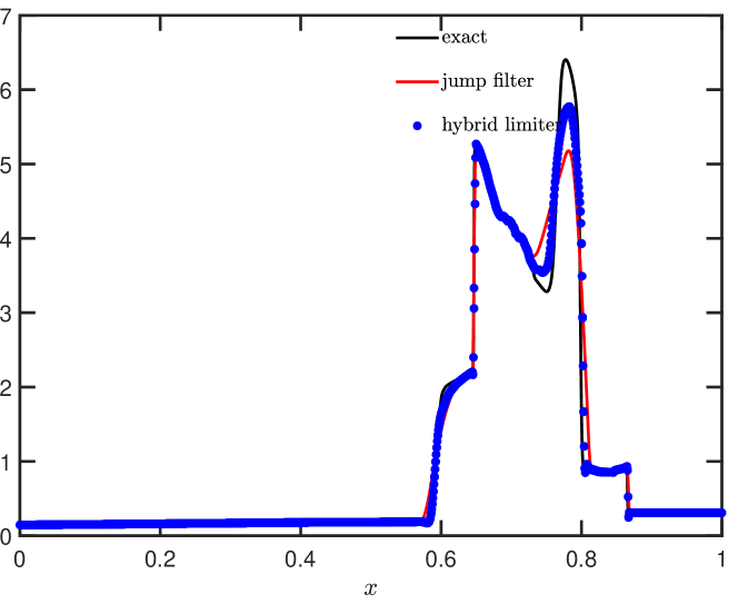
Example 3.3 (Blast waves).
We then consider the interaction of two blast waves with the initial condition:
| (3.49) |
Reflecting boundary conditions are applied at both endpoints, and the numerical solutions are depicted in Figs. 3.2. Here, the “exact” solution refers to the numerical solution computed by the fifth-order finite difference WENOZ-H scheme [76] with grid points. Initially, it’s evident that the DG scheme with the jump filter maintains sharp, oscillation-free resolution near shocks. To further minimize numerical dissipation, we employ the hybrid limiter associated with the jump filter for this problem. Comparing the results, we observe that the hybrid limiter exhibits superior resolution compared to the DG scheme with the jump filter alone.

Example 3.4 (Shu-Osher shock tube problem).
Next, we consider the shock density wave interaction problem with a moving Mach 3 shock interacting with sine waves in the density:
| (3.50) |
Given that this solution exhibits both shocks and a complex smooth region structure, a higher-order scheme is expected to showcase its advantages. For reference, the “exact” solution is computed using the fifth-order finite difference WENO scheme [39] with 2000 grid points. In Figs. 3.3, the density is plotted using the DG method with the jump filter and the hybrid limiter associated with it. Both schemes effectively capture high-frequency waves, and the hybrid limiter demonstrates its ability to efficiently reduce numerical dissipation. Additionally, higher-order DG methods with the jump filter or the hybrid limiter outperform their lower-order counterparts.


3.2 Two dimensional tests
The 2D Euler equation can be written as:
| (3.51) |
with , , where , , and . Here, represents density, and and are velocities and momenta. is the total energy, is pressure, and is the internal energy. And is the ratio of specific heats. Unless otherwise specified, we always take . For Euler equations in 2D, the damping term (2.41) serves to determine the magnitude of the viscosity term with in (2.42), where and are the estimates of the local maximum wave speeds in the - and -directions, respectively.
Example 3.5 (Vortex evolution problems).
We now consider the problem of vortex evolution. An isentropic vortex perturbation centered at is added to the velocity , temperature (), and entropy () of the flow, given in the following:
where , , and the . Here is the strength of the vortex, controls the decay rate of the vortex, and is the critical radius at which the vortex has the maximum strength. We test the following two cases:
-
(a)
(accuracy test) The state of the mean flow is given by . The parameters are taken as , , , . The exact solution represents the convection motion of the vortex with the mean flow velocity. We compute the numerical solution at time in the region under periodic boundary conditions. Table 3.2 presents the accuracy and convergence rates. It is observed that the DG scheme with the jump filter achieves the expected convergence rate, surpassing . This deviation is attributed to the dominance of the viscous term on coarse meshes. However, with mesh refinement, the convergence rate rapidly approaches the theoretically expected order of accuracy. Moreover, comparison with the standard DG scheme reveals negligible differences in errors on fine meshes, suggesting a minimal impact of our jump filter as expected. As the mesh is refined, the jumps between adjacent cells diminish significantly.
-
(b)
(shock-vortex interaction) The model problem characterizes the mutual interference effects of a stationary shock wave and a moving vortex. The computational domain is given by . A stationary shock wave is located at and is perpendicular to the -axis. The left state of the shock wave is . A small vortex is imposed on the fluid to the left of the shock wave, with its center at . We take the same values of these parameters as in [39] that , , and . The upper and lower boundaries are subjected to reflective boundary conditions. Figure 3.4 displays contour plots of pressure at six distinct times, illustrating the shock-vortex interaction dynamics. Employing DG schemes with the jump filter effectively captures these dynamics and accurately depicts intricate wave structures. The obtained results are comparable to those reported in [39].
| results with filter | results without filter | ||||||||
| error | order | error | order | error | order | error | order | ||
| 6.26e-03 | – | 6.79e-02 | – | 1.30e-03 | – | 1.60e-02 | – | ||
| 5.52e-04 | 3.50 | 4.97e-03 | 3.77 | 1.93e-04 | 2.75 | 2.25e-03 | 2.83 | ||
| 4.70e-05 | 3.55 | 4.90e-04 | 3.33 | 2.84e-05 | 2.76 | 3.74e-04 | 2.58 | ||
| 5.70e-06 | 3.04 | 7.48e-05 | 2.71 | 4.96e-06 | 2.52 | 8.37e-05 | 2.16 | ||
| 1.08e-06 | 2.39 | 1.85e-05 | 2.01 | 1.06e-06 | 2.22 | 1.97e-05 | 2.08 | ||
| 1.23e-03 | – | 1.32e-02 | – | 2.06e-05 | – | 5.76e-04 | – | ||
| 3.13e-05 | 5.29 | 3.55e-04 | 5.21 | 2.77e-06 | 2.89 | 7.24e-05 | 2.99 | ||
| 1.01e-06 | 4.94 | 1.49e-05 | 4.57 | 3.88e-07 | 2.83 | 9.64e-06 | 2.90 | ||
| 6.21e-08 | 4.03 | 1.21e-06 | 3.61 | 5.36e-08 | 2.85 | 1.33e-06 | 2.85 | ||
| 7.46e-09 | 3.05 | 1.92e-07 | 2.70 | 7.37e-09 | 2.86 | 1.97e-07 | 2.75 | ||
| 1.65e-03 | – | 1.83e-02 | – | 6.47e-07 | – | 1.38e-05 | – | ||
| 1.72e-06 | 9.90 | 3.48e-05 | 9.04 | 3.33e-08 | 4.28 | 9.25e-07 | 3.90 | ||
| 2.13e-08 | 6.33 | 3.42e-07 | 6.66 | 1.86e-09 | 4.16 | 5.45e-08 | 4.08 | ||
| 3.49e-10 | 5.93 | 7.18e-09 | 5.57 | 1.10e-10 | 4.08 | 3.18e-09 | 4.10 | ||
| 8.66e-12 | 5.33 | 2.37e-10 | 4.92 | 6.82e-12 | 4.01 | 1.85e-10 | 4.10 | ||


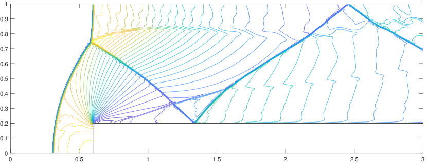
Example 3.6 (Double Mach reflection problem).
This is a benchmark test for the two-dimensional Euler equations for high-resolution schemes. The computation domain is . A right-moving Mach shock is located at , , making a angle with the horizontal wall. At the top boundary, the flow values are set to describe the exact motion of the Mach 10 shock. The boundary conditions at the left and the right are inflow and outflow respectively.
The contour plots of density in DG solutions with the jump filter and the hybrid limiter at time are presented in Figs. 3.5, with zoomed-in views in Figs. 3.6. Firstly, it’s evident that the DG scheme with the jump filter effectively captures shock waves, with resolution improving as accuracy increases. These results mirror the effect of TVB limiters in achieving total variation boundedness in standard DG schemes [13], as further explored in [77].
On the other hand, when utilizing the hybrid limiter associated with the jump filter as lower-order limiters, the scheme adeptly captures shock waves and showcases the advantages of higher-order schemes more comprehensively. Higher-order schemes exhibit superior resolution, particularly below the Mach stem, as illustrated in Figs. 3.6. This underscores that employing the jump filter as lower-order polynomials in the hybrid limiter not only facilitates efficient capture of shock waves but also minimizes numerical dissipation.


Example 3.7 (Forward facing step problem).
The wind tunnel is units in length and unit in width, and the step is units high, located units from the left end of the tunnel. The initial condition is a uniform flow given by . Reflective boundary conditions are applied along the wall boundaries, and inflow and outflow boundary conditions are imposed along the left and right boundaries.
The DG solutions with the jump filter and the associated hybrid limiter are depicted in Figs. 3.7 at time . Notably, all schemes exhibit essential oscillation-free behavior. Additionally, a discernible difference emerges between higher and lower-order schemes: the former more effectively captures slip lines, showcasing the superiority of higher-order schemes. Moreover, employing the hybrid approach yields even lower dissipation. This can be attributed to its ability to effectively capture the intricate flow structure and resolve slip lines better than the jump filter alone.


Example 3.8 (Shock passing a backward facing corner).
Shock diffraction is a very common phenomenon. The computational domain for this problem is and . The initial condition is a pure right-moving shock of Mach , initially located at and , moving into undisturbed air ahead of the shock with . We use the inflow boundary condition at , reflective boundary condition at and , and outflow boundary condition elsewhere. To ensure the positivity of the density and pressure of the DG solutions, we first apply the jump filter, and then we utilize the positivity-preserving (PP) limiter introduced by Zhang and Shu [82] in Examples 3.8 and 3.9. Due to the conservation nature of our scheme, integrating the PP limiter is straightforward. Based on our numerical tests, we’ve found that the DG scheme with the jump filter can maintain positivity even without PP limiters for certain grid configurations. However, this isn’t universally true. Figures 3.8 depict density contour plots at time . Evidently, all schemes successfully exhibit the essential property of non-oscillation in the numerical solution. Furthermore, the higher-order scheme consistently outperforms the lower-order scheme in accurately capturing the slip line.


Example 3.9 (High Mach number astrophysical jets).
We consider the high Mach number astrophysical jets without the radiative cooling [82]. A Mach problem is considered to show the robustness of the scheme with the PP limiter [82]. The computational domain is taken as , initially full of the ambient gas with . The right, top, and bottom boundary are outflows. For the left boundary, if and otherwise. The numerical solution at a mesh of is shown in Figs. 3.10. We can observe that the numerical results closely resemble the corresponding outcomes in [82].


Example 3.10 (Shock-bubble interaction).
In this experiment we simulate a strong rightwards moving shock wave over a low density gas bubble [8]. The computational domain is . At the initial time, the region exhibits three different states: (A) ; (B) a circular disk centered at with a radius of ; (C) other regions. In region (A), . In region (B), . In region (C), . The left boundary has the Dirichlet boundary condition, the right has the outflow boundary condition, and the top and bottom boundaries have the solid wall boundary condition. In this example, a moving shockwave propagates to the right and compresses the bubble in the region (B). In the left of Figs. 3.11, we present numerical results obtained with different schemes at , and in the right Figs. 3.11, we display the density distribution around the bubble. It can be observed that the higher-order schemes with the jump filter capture more unstable and intricate structures, providing a more detailed representation of the flow field.


Example 3.11 (Kelvin-Helmholtz (KH) instability).
The KH instability problem is considered in a computational domain of . The initial values within this domain are set as follows:
where . Periodic boundary conditions are applied and the simulation concludes at . Figures 3.12 depict the density distribution obtained using the jump filter with and basis functions. Noticeably, the higher-order schemes generate more intricate vortex structures and turbulent mixing layers.


4 Conclusions
By incorporating a local viscosity term based solely on cell interface jumps, this paper introduces a novel shock capturing approach to the DG scheme. This scheme is efficiently implemented through a splitting fashion without impacting the chosen time step. Its favorable properties are ensured by rigorous mathematical theory, guaranteeing conservation, stability, and optimal error estimation. Extensive numerical experiments, primarily focusing on various test cases of the Euler equations, validate the proposed method, showcasing its efficacy in controlling numerical spurious oscillations, particularly in scenarios involving strong shock waves. Furthermore, by integrating the novel jump filter into a hybrid limiter framework, the scheme effectively suppresses numerical spurious oscillations while further reducing dissipation. The jump filter maintains the compactness of the DG scheme, facilitating easy implementation and enabling efficient parallel computations. An important advantage of this approach is its simplicity and computational efficiency. For each time step, only the multiplication of the coefficients by a precomputed factor is necessary. This factor is calculated in physical space without the need for characteristic decomposition. It appears that the jump filter can be seamlessly implemented on unstructured meshes, and we plan to explore this capability and its application in steady-state problems in our future work to enhance its versatility and applicability.
5 Appendix
In this section, we provide the proof of Theorem 2.1. Before presenting the proof, we provide some preliminary knowledge. The Gauss-Radau projection provides great help in obtaining the optimal error estimates. For any function , the projection is defined as the unique element in such that
By a standard scaling argument [10], it is easy to obtain the following approximation property:
| (5.52) |
here the constant is independent of and and . In addition, the following inverse property with respect to the finite element space will be used in our analysis.
| (5.53) | ||||
Now we present several properties of the DG operator defined by (2.26). The proofs are routine, so we omit them to save space.
| (5.54) | |||
| (5.55) |
where and .
To obtain the error equation, we first present the local truncation error in time for the exact functions. Suppose the exact solution is smooth enough, then we have
| (5.56) |
and . Let and denote , . Multiplying the test function on both sides of (5.56) and integrating by parts yields the following equality
| (5.57) |
As the usual treatment, define
Subtracting (5.57) from the scheme (2.27) with gives the error equation
| (5.58) |
here we have used the property (5.55). Obviously, we have the following equivalent form
| (5.59) |
To obtain the final error estimate for the scheme (2.27)-(2.28), we would like to give the following lemmas. In what follows, we use to represent a generic positive constant that is independent of , , and . It may have a different value in each occurrence.
Lemma 5.1.
Proof.
By the smoothness of the exact solution and the linearity of the projection , it follows from (5.52) that the projection error and its evolution satisfies
| (5.60) |
The proposition can be proven by noting that . ∎
Lemma 5.2.
Under the CFL condition , we have
Proof.
Lemma 5.3.
Suppose is defined by (2.7), then we have
Proof.
By the jump viscosity coefficient and the smoothness of the exact solution, we get
here we have used the inverse inequalities (5.53). Thus we have
∎
We make an a priori assumption for all
| (5.61) |
and it will be verified in the end. Now we can obtain the following the error estimates.
Lemma 5.4.
If , then we have
Proof.
If , then holds for any . Note that is independent of and satisfies (2.28). The following error equation holds
Taking yields
Since the second term on the left is nonnegative, we have
Here we have used Lemma 5.3, and the inverse estimate (5.53). Applying the property (5.60), we get
Integrating the inequality from to and using , , we derive
The proof is completed by using the estimate of in Lemma 5.2. ∎
Now we can give the proof of Theorem 2.1.
Proof of 2.1.
Along the same lines to prove the stability of the RKDG scheme [80], taking in the error equation (5.59) and using the property (5.54), we have
| (5.62) |
here we have used the estimates in Lemma 5.1 and 5.4. Then apply the discrete Gronwall inequality to get
A simple use of the triangle inequality, the approximation property of and the fact that , we have . Thus
The proof is completed by the triangle inequality and the approximation property of . ∎
In the end, we will verify the a prior assumption (5.61). Note that and . Then , hold for with and a priori assumption holds for . By Lemma 5.2 and the CFL condition with , we have . Thus a priori assumption holds for . By Lemma 5.4 and (5.62), we have . This argument can be further continued and formalized by induction to show that and for any . This validates the a priori assumption (5.61).
References
- [1] H. Abbassi, F. Mashayek, and G.B. Jacobs. Shock capturing with entropy-based artificial viscosity for staggered grid discontinuous spectral element method. Comput. & Fluids, 98:152–163, 2014.
- [2] G. Barter and D. Darmofal. Shock capturing with higher-order, PDE-based artificial viscosity. In 18th AIAA Computational Fluid Dynamics Conference, page 3823, 2007.
- [3] F. Bassi, A. Crivellini, A. Ghidoni, and S. Rebay. High-order discontinuous Galerkin discretization of transonic turbulent flows. In 47th AIAA aerospace sciences meeting including the new horizons forum and aerospace exposition, page 180, 2009.
- [4] A. Bhagatwala and S.K. Lele. A modified artificial viscosity approach for compressible turbulence simulations. J. Comput. Phys., 228(14):4965–4969, 2009.
- [5] R. Biswas, K.D. Devine, and J. Flaherty. Parallel, adaptive finite element methods for conservation laws. Appl. Numer. Math., 14(1-3):255–283, 1994.
- [6] A. Burbeau, P. Sagaut, and Ch.-H. Bruneau. A problem-independent limiter for high-order Runge-Kutta discontinuous Galerkin methods. J. Comput. Phys., 169(1):111–150, 2001.
- [7] E. Burman. On nonlinear artificial viscosity, discrete maximum principle and hyperbolic conservation laws. BIT Numerical Mathematics, 47:715–733, 2007.
- [8] M. Cada and M. Torrilhon. Compact third-order limiter functions for finite volume methods. J. Comput. Phys., 228(11):4118–4145, 2009.
- [9] A. Chaudhuri, G.B. Jacobs, W.-S. Don, H Abbassi, and F. Mashayek. Explicit discontinuous spectral element method with entropy generation based artificial viscosity for shocked viscous flows. J. Comput. Phys., 332:99–117, 2017.
- [10] P.G. Ciarlet. The finite element method for elliptic problems, volume 40 of Classics in Applied Mathematics. Society for Industrial and Applied Mathematics (SIAM), Philadelphia, PA.
- [11] B. Cockburn, S.-Y. Lin, and C.-W. Shu. TVB Runge-Kutta local projection discontinuous Galerkin finite element method for conservation laws III: one-dimensional systems. J. Comput. Phys., 84(1):90–113, 1989.
- [12] B. Cockburn and C.-W. Shu. TVB Runge-Kutta local projection discontinuous Galerkin finite element method for conservation laws. II. General framework. Math. Comput., 52(186):411–435, 1989.
- [13] B. Cockburn and C.-W. Shu. The Runge-Kutta discontinuous Galerkin method for conservation laws V: multidimensional systems. J. Comput. Phys., 141(2):199–224, 1998.
- [14] A.W. Cook and W.H. Cabot. A high-wavenumber viscosity for high-resolution numerical methods. J. Comput. Phys., 195(2):594–601, 2004.
- [15] A.W. Cook and W.H. Cabot. Hyperviscosity for shock-turbulence interactions. J. Comput. Phys., 203(2):379–385, 2005.
- [16] W.-S. Don, D. Gottlieb, and J.-H. Jung. A multidomain spectral method for supersonic reactive flows. J. Comput. Phys., 192(1):325–354, 2003.
- [17] W.S. Don. Numerical study of pseudospectral methods in shock wave applications. J. Comput. Phys., 110(1):103–111, 1994.
- [18] P. Fernandez, C. Nguyen, and J. Peraire. A physics-based shock capturing method for unsteady laminar and turbulent flows. In 2018 AIAA Aerospace Sciences Meeting, page 0062, 2018.
- [19] B. Fiorina and S.K. Lele. An artificial nonlinear diffusivity method for supersonic reacting flows with shocks. J. Comput. Phys., 222(1):246–264, 2007.
- [20] D. Gottlieb and J.S. Hesthaven. Spectral methods for hyperbolic problems. J. Comput. Appl. Math., 128(1-2):83–131, 2001.
- [21] S. Gottlieb, C.-W. Shu, and E. Tadmor. Strong stability-preserving high-order time discretization methods. SIAM Rev., 43:89–112, 2001.
- [22] J.-L. Guermond and R. Pasquetti. Entropy-based nonlinear viscosity for Fourier approximations of conservation laws. C. R. Math. Acad. Sci. Paris, 346(13-14):801–806, 2008.
- [23] J.-L. Guermond, R. Pasquetti, and B. Popov. Entropy viscosity method for nonlinear conservation laws. J. Comput. Phys., 230(11):4248–4267, 2011.
- [24] A. Harten, B. Engquist, S. Osher, and S. Chakravarthy. Uniformly high order accurate essentially non-oscillatory schemes, iii. J. Comput. Phys., 131(1):3–47, 1987.
- [25] A. Harten, P.D. Lax, and B. Van Leer. On upstream differencing and godunov-type schemes for hyperbolic conservation laws. SIAM Rev, 25(1):35–61, 1983.
- [26] R. Hartmann. Adaptive discontinuous Galerkin methods with shock-capturing for the compressible Navier-Stokes equations. Internat. J. Numer. Methods Fluids, 51(9-10):1131–1156, 2006.
- [27] R. Hartmann. Higher-order and adaptive discontinuous Galerkin methods with shock-capturing applied to transonic turbulent delta wing flow. Internat. J. Numer. Methods Fluids, 72(8):883–894, 2013.
- [28] R. Hartmann and P. Houston. Adaptive discontinuous Galerkin finite element methods for the compressible Euler equations. J. Comput. Phys., 183(2):508–532, 2002.
- [29] J.S. Hesthaven. Numerical methods for conservation laws: From analysis to algorithms. SIAM, 2017.
- [30] J.S. Hesthaven and R. Kirby. Filtering in Legendre spectral methods. Math. Comput., 77(263):1425–1452, 2008.
- [31] J.S. Hesthaven and T. Warburton. Nodal discontinuous Galerkin methods: algorithms, analysis, and applications. Springer Science & Business Media, 2007.
- [32] A. Hiltebrand and S. Mishra. Entropy stable shock capturing space–time discontinuous galerkin schemes for systems of conservation laws. Numerische Mathematik, 126:103–151, 2014.
- [33] S. Hou and X.D. Liu. Solutions of multi-dimensional hyperbolic systems of conservation laws by square entropy condition satisfying discontinuous Galerkin method. J. Sci. Comput., 31:127–151, 2007.
- [34] T. J. R. Hughes and T. E. Tezduyar. Finite element methods for first-order hyperbolic systems with particular emphasis on the compressible Euler equations. Comput. Methods Appl. Mech. Engrg., 45(1-3):217–284, 1984.
- [35] A. Jameson. Artificial diffusion, upwind biasing, limiters and their effect on accuracy and multigrid convergence in transonic and hypersonic flows. In 11th Computational Fluid Dynamics Conference, page 3359, 1993.
- [36] A. Jameson. A perspective on computational algorithms for aerodynamic analysis and design. Progress in Aerospace Sciences, 37(2):197–243, 2001.
- [37] A. Jameson, W. Schmidt, and E. Turkel. Numerical solution of the Euler equations by finite volume methods using Runge Kutta time stepping schemes. In 14th fluid and plasma dynamics conference, page 1259, 1981.
- [38] G.-S. Jiang and C.-W. Shu. On a cell entropy inequality for discontinuous Galerkin methods. Math. Comput., 62(206):531–538, 1994.
- [39] G.-S. Jiang and C.-W. Shu. Efficient implementation of weighted ENO schemes. J. Comput. Phys., 126(1):202–228, 1996.
- [40] G-S. Karamanos and G.E. Karniadakis. A spectral vanishing viscosity method for large-eddy simulations. J. Comput. Phys., 163(1):22–50, 2000.
- [41] S. Kawai and S.K. Lele. Localized artificial diffusivity scheme for discontinuity capturing on curvilinear meshes. J. Comput. Phys., 227(22):9498–9526, 2008.
- [42] A. Klöckner, T. Warburton, J. Bridge, and J.S. Hesthaven. Nodal discontinuous galerkin methods on graphics processors. J. Comput. Phys., 228(21):7863–7882, 2009.
- [43] L. Krivodonova. Limiters for high-order discontinuous Galerkin methods. J. Comput. Phys., 226(1):879–896, 2007.
- [44] D. Kuzmin. A vertex-based hierarchical slope limiter for p-adaptive discontinuous Galerkin methods. J. Comput. Appl. Math., 233(12):3077–3085, 2010.
- [45] D. Kuzmin. Slope limiting for discontinuous Galerkin approximations with a possibly non-orthogonal Taylor basis. Internat. J. Numer. Methods Fluids, 71(9):1178–1190, 2013.
- [46] D. Kuzmin. Hierarchical slope limiting in explicit and implicit discontinuous Galerkin methods. J. Comput. Phys., 257:1140–1162, 2014.
- [47] Randall J. LeVeque. Numerical methods for conservation laws. Lectures in Mathematics ETH Zürich. Birkhäuser Verlag, Basel, second edition, 1992.
- [48] X.-D. Liu, S. Osher, and T. Chan. Weighted essentially non-oscillatory schemes. J. Comput. Phys., 115(1):200–212, 1994.
- [49] Y. Liu, J. Lu, and C.-W. Shu. An essentially oscillation-free discontinuous Galerkin method for hyperbolic systems. SIAM J. Sci. Comput., 44(1):A230–A259, 2022.
- [50] Y. Liu, M. Vinokur, and Z. Wang. Spectral difference method for unstructured grids I: Basic formulation. J. Comput. Phys., 216(2):780–801, 2006.
- [51] G. Lodato. Characteristic modal shock detection for discontinuous finite element methods. Comput. & Fluids, 179:309–333, 2019.
- [52] J. Lu, Y. Liu, and C.-W. Shu. An oscillation-free discontinuous Galerkin method for scalar hyperbolic conservation laws. SIAM J. Numer. Anal., 59(3):1299–1324, 2021.
- [53] H. Luo, J.D. Baum, and R. Löhner. A Hermite WENO-based limiter for discontinuous Galerkin method on unstructured grids. J. Comput. Phys., 225(1):686–713, 2007.
- [54] Y. Lv, Y. See, and M. Ihme. An entropy-residual shock detector for solving conservation laws using high-order discontinuous Galerkin methods. J. Comput. Phys., 322:448–472, 2016.
- [55] Y. Maday, S.M.O. Kaber, and E. Tadmor. Legendre pseudospectral viscosity method for nonlinear conservation laws. SIAM J. Numer. Anal., 30(2):321–342, 1993.
- [56] J. Markert, G. Gassner, and S. Walch. A sub-element adaptive shock capturing approach for discontinuous Galerkin methods. Commun. Appl. Math. Comput., 5(2):679–721, 2023.
- [57] A. Meister, S. Ortleb, and Th. Sonar. Application of spectral filtering to discontinuous Galerkin methods on triangulations. Numer. Methods Partial Differential Equations, 28(6):1840–1868, 2012.
- [58] N.-A. Messaï, G. Daviller, and J.-F. Boussuge. Artificial viscosity-based shock capturing scheme for the Spectral Difference method on simplicial elements. J. Comput. Phys., 504:Paper No. 112864, 31, 2024.
- [59] David Moro, Ngoc Cuong Nguyen, and Jaime Peraire. Dilation-based shock capturing for high-order methods. Internat. J. Numer. Methods Fluids, 82(7):398–416, 2016.
- [60] M. Nazarov and J. Hoffman. Residual-based artificial viscosity for simulation of turbulent compressible flow using adaptive finite element methods. Internat. J. Numer. Methods Fluids, 71(3):339–357, 2013.
- [61] P.O. Persson. Shock capturing for high-order discontinuous Galerkin simulation of transient flow problems. In 21st AIAA computational fluid dynamics conference, page 3061, 2013.
- [62] P.O. Persson and J. Peraire. Sub-cell shock capturing for discontinuous Galerkin methods. In 44th AIAA aerospace sciences meeting and exhibit, page 112, 2006.
- [63] S. Premasuthan, C. Liang, and A. Jameson. Computation of flows with shocks using the spectral difference method with artificial viscosity, I: basic formulation and application. Comput. & Fluids, 98:111–121, 2014.
- [64] S. Premasuthan, C. Liang, and A. Jameson. Computation of flows with shocks using the spectral difference method with artificial viscosity, II: modified formulation with local mesh refinement. Comput. & Fluids, 98:122–133, 2014.
- [65] J. Qiu and C.-W. Shu. Runge-Kutta discontinuous Galerkin method using WENO limiters. SIAM J. Sci. Comput., 26(3):907–929, 2005.
- [66] V. Shankar, G.B. Wright, and A. Narayan. A robust hyperviscosity formulation for stable RBF-FD discretizations of advection-diffusion-reaction equations on manifolds. SIAM J. Sci. Comput., 42(4):A2371–A2401, 2020.
- [67] C.-W. Shu. Discontinuous Galerkin method for time-dependent problems: survey and recent developments. Recent developments in discontinuous Galerkin finite element methods for partial differential equations, pages 25–62, 2014.
- [68] M. Sonntag and C. Munz. Efficient parallelization of a shock capturing for discontinuous Galerkin methods using finite volume sub-cells. J. Sci. Comput., 70(3):1262–1289, 2017.
- [69] E. Tadmor. Convergence of spectral methods for nonlinear conservation laws. SIAM J. Numer. Anal., 26(1):30–44, 1989.
- [70] E. Tadmor. Super-viscosity and spectral approximations of nonlinear conservation laws. In Numerical methods for fluid dynamics, 4 (Reading, 1992), pages 69–81. Oxford Univ. Press, New York, 1993.
- [71] I. Tominec and M. Nazarov. Residual viscosity stabilized RBF-FD methods for solving nonlinear conservation laws. J. Sci. Comput., 94(1):Paper No. 14, 31, 2023.
- [72] N. Tonicello, G. Lodato, and L. Vervisch. Entropy preserving low dissipative shock capturing with wave-characteristic based sensor for high-order methods. Comput. & Fluids, 197:104357, 17, 2020.
- [73] E.F. Toro. Riemann solvers and numerical methods for fluid dynamics: a practical introduction. Springer Science & Business Media, 2013.
- [74] H. Vandeven. Family of spectral filters for discontinuous problems. J. Sci. Comput., 6(2):159–192, 1991.
- [75] J. Von Neumann and R. D. Richtmyer. A method for the numerical calculation of hydrodynamic shocks. J. Appl. Phys., 21:232–237, 1950.
- [76] Y. Wan and Y. Xia. A new hybrid WENO scheme with the high-frequency region for hyperbolic conservation laws. Commun. Appl. Math. Comput., 5(1):199–234, 2023.
- [77] L. Wei and Y. Xia. An indicator-based hybrid limiter in discontinuous Galerkin methods for hyperbolic conservation laws. J. Comput. Phys., 498:Paper No. 112676, 25, 2024.
- [78] Y. Xu, X. Meng, C.-W. Shu, and Q. Zhang. Superconvergence analysis of the Runge-Kutta discontinuous Galerkin methods for a linear hyperbolic equation. J. Sci. Comput., 84(1):Paper No. 23, 40, 2020.
- [79] Y. Xu, C.-W. Shu, and Q. Zhang. Error estimate of the fourth-order Runge-Kutta discontinuous Galerkin methods for linear hyperbolic equations. SIAM J. Numer. Anal., 58(5):2885–2914, 2020.
- [80] Y. Xu, Q. Zhang, C.-W. Shu, and H. Wang. The -norm stability analysis of Runge-Kutta discontinuous Galerkin methods for linear hyperbolic equations. SIAM J. Numer. Anal., 57(4):1574–1601, 2019.
- [81] J. Yu and J.S. Hesthaven. A study of several artificial viscosity models within the discontinuous Galerkin framework. Commun. Comput. Phys., 27(5):1309–1343, 2020.
- [82] X. Zhang and C.-W. Shu. On positivity-preserving high order discontinuous Galerkin schemes for compressible Euler equations on rectangular meshes. J. Comput. Phys., 229(23):8918–8934, 2010.
- [83] X. Zhong and C.-W. Shu. A simple weighted essentially nonoscillatory limiter for Runge-Kutta discontinuous Galerkin methods. J. Comput. Phys., 232(1):397–415, 2013.
- [84] J. Zhu, J. Qiu, and C.-W. Shu. High-order Runge-Kutta discontinuous Galerkin methods with a new type of multi-resolution WENO limiters. J. Comput. Phys., 404:109105, 18, 2020.
- [85] J. Zhu, J. Qiu, C.-W. Shu, and M. Dumbser. Runge–Kutta discontinuous Galerkin method using WENO limiters II: unstructured meshes. J. Comput. Phys., 227(9):4330–4353, 2008.
- [86] V. Zingan, J.-L. Guermond, J. Morel, and B. Popov. Implementation of the entropy viscosity method with the discontinuous Galerkin method. Comput. Methods Appl. Mech. Engrg., 253:479–490, 2013.