The Interpolation Phase Transition in Neural Networks:
Memorization and Generalization under Lazy Training

Andrea Montanari and Yiqiao Zhong¹¹footnotemark: 1 Department of Electrical Engineering and Department of Statistics, Stanford University

Abstract

Modern neural networks are often operated in a strongly overparametrized regime: they comprise so many parameters that they can interpolate the training set, even if actual labels are replaced by purely random ones. Despite this, they achieve good prediction error on unseen data: interpolating the training set does not lead to a large generalization error. Further, overparametrization appears to be beneficial in that it simplifies the optimization landscape. Here we study these phenomena in the context of two-layers neural networks in the neural tangent (NT) regime. We consider a simple data model, with isotropic covariates vectors in $d$ dimensions, and $N$ hidden neurons. We assume that both the sample size $n$ and the dimension $d$ are large, and they are polynomially related. Our first main result is a characterization of the eigenstructure of the empirical NT kernel in the overparametrized regime $Nd\gg n$ . This characterization implies as a corollary that the minimum eigenvalue of the empirical NT kernel is bounded away from zero as soon as $Nd\gg n$ , and therefore the network can exactly interpolate arbitrary labels in the same regime.

Our second main result is a characterization of the generalization error of NT ridge regression including, as a special case, min- $\ell_{2}$ norm interpolation. We prove that, as soon as $Nd\gg n$ , the test error is well approximated by the one of kernel ridge regression with respect to the infinite-width kernel. The latter is in turn well approximated by the error of polynomial ridge regression, whereby the regularization parameter is increased by a ‘self-induced’ term related to the high-degree components of the activation function. The polynomial degree depends on the sample size and the dimension (in particular on $\log n/\log d$ ).

1 Introduction

Tractability and generalization are two key problems in statistical learning. Classically, tractability is achieved by crafting suitable convex objectives, and generalization by regularizing (or restricting) the function class of interest to guarantee uniform convergence. In modern neural networks, a different mechanism appears to be often at work [NTS15, ZBH⁺16, BHMM19]. Empirical risk minimization becomes tractable despite non-convexity because the model is overparametrized. In fact, so overparametrized that a model interpolating perfectly the training set is found in the neighborhood of most initializations. Despite this, the resulting model generalizes well to unseen data: the inductive bias produced by gradient-based algorithms is sufficient to select models that generalize well.

Elements of this picture have been rigorously established in special regimes. In particular, it is known that for neural networks with a sufficiently large number of neurons, gradient descent converges quickly to a model with vanishing training error [DZPS18, AZLS19, OS20]. In a parallel research direction, the generalization properties of several examples of interpolating models have been studied in detail [BLLT20, LR20, HMRT19, BHX19, MM21, MRSY19]. The present paper continues along the last direction, by studying the generalization properties of linear interpolating models that arise from the analysis of neural networks.

In this context, many fundamental questions remain challenging. (We refer to Section 4 for pointers to recent progress on these questions.)

Q1.

When is a neural network sufficiently complex to interpolate $n$ data points? Counting degrees of freedom would suggest that this happens as soon as the number of parameters in the network is larger than $n$ . Does this lower bound predict the correct threshold? What are the architectures that achieve this lower bound?
Q2.

Assume that the answer to the previous question is positive, namely a network with the order of $n$ parameters can interpolate $n$ data points. Can such a network be found efficiently, using standard gradient descent (GD) or stochastic gradient descent (SGD)?
Q3.

Can we characterize the generalization error above this interpolation threshold? Does it decrease with the number of parameters? What is the nature of the implicit regularization and of the resulting model $\widehat{f}(\text{\boldmath$x$})$ ?

Here we address these questions by studying a class of linear models known as ‘neural tangent’ models. Our focus will be on characterizing test error and generalization, i.e., on the last question Q3, but our results are also relevant to Q1 and Q2.

We assume to be given data $\{(\text{\boldmath$x$}_{i},y_{i})\}_{i\leq n}$ with i.i.d. $d$ -dimensional covariates vectors $\text{\boldmath$x$}_{i}\sim\mathrm{Unif}(\mathbb{S}^{d-1}(\sqrt{d}))$ (we denote by $\mathbb{S}^{d-1}(r)$ the sphere of radius $r$ in $d$ dimensions). In addressing questions Q1 and Q2, we assume the labels $y_{i}$ to be arbitrary. For Q3 we will assume $y_{i}=f_{*}(\text{\boldmath$x$}_{i})+\varepsilon_{i}$ , where $\varepsilon_{1},\ldots,\varepsilon_{n}$ are independent noise variables with $\mathbb{E}(\varepsilon_{i})=0$ and $\mathbb{E}(\varepsilon^{2}_{i})=\sigma_{\varepsilon}^{2}$ . Crucially, we allow for a general target function $f_{*}$ under the minimal condition $\mathbb{E}\{f_{*}(\text{\boldmath$x$}_{i})^{2}\}<\infty$ . We assume both the dimension and sample size to be large and polynomially related, namely $c_{0}d\leq n\leq d^{1/c_{0}}$ for some small constant $c_{0}$ .

A substantial literature [DZPS18, AZLS19, ZCZG20, OS20, LZB20] shows that, under certain training schemes, multi-layer neural networks can be well approximated by linear models with a nonlinear (randomized) featurization map that depends on the network architecture and its initialization. In this paper, we will focus on the simplest such models. Given a set of weights $\text{\boldmath$W$}=(\text{\boldmath$w$}_{1},\dots,\text{\boldmath$w$}_{N})$ , we define the following function class with $Nd$ parameters $\text{\boldmath$a$}:=(\text{\boldmath$a$}_{1},\dots,\text{\boldmath$a$}_{N})$ :

\displaystyle\mathcal{F}_{{\sf NT}}^{N}(\text{\boldmath$W$}):=\Big{\{}f(\text{\boldmath$x$};\text{\boldmath$a$}):=\frac{1}{\sqrt{Nd}}\sum_{i=1}^{N}\langle\text{\boldmath$a$}_{i},\text{\boldmath$x$}\rangle\sigma^{\prime}(\langle\text{\boldmath$w$}_{i},\text{\boldmath$x$}\rangle)\,\;\;\;\text{\boldmath$a$}_{i}\in\mathbb{R}^{d}\Big{\}}\,.

(1)

In other words, to a vector of covariates $\text{\boldmath$x$}\in\mathbb{R}^{d}$ , the NT model associates a (random) features vector

\text{\boldmath$\Phi$}(\text{\boldmath$x$})=\frac{1}{\sqrt{Nd}}[\sigma^{\prime}(\langle\text{\boldmath$x$},\text{\boldmath$w$}_{1}\rangle)\text{\boldmath$x$}^{\sf T},\ldots,\sigma^{\prime}(\langle\text{\boldmath$x$},\text{\boldmath$w$}_{N}\rangle)\text{\boldmath$x$}^{\sf T}]\in\mathbb{R}^{Nd}.

(2)

The model then computes a linear function $f(\text{\boldmath$x$};\text{\boldmath$a$})=\langle\text{\boldmath$a$},\text{\boldmath$\Phi$}(\text{\boldmath$x$})\rangle$ . We fit the parameters $a$ via minimum $\ell_{2}$ -norm interpolation:

	minimize	$\displaystyle\;\;\;\;\\|\text{\boldmath$a$}\\|_{2}\,,$		(3)
	subj. to	$\displaystyle\;\;\;\;f(\text{\boldmath$x$}_{i};\text{\boldmath$a$})=y_{i}\;\;\;\forall i\leq n\,.$		(3)

We will also study a generalization of min $\ell_{2}$ -norm interpolation which is given by least-squares regression with ridge penalty. Interpolation is recovered in the limit in which the ridge parameter tends to $0$ .

As mentioned, the construction of model (1) and the choice of minimum $\ell_{2}$ -norm interpolation (3) are motivated by the analysis of two-layers neural networks. In a nutshell, for a suitable scaling of the initialization, two-layer networks trained via gradient descent are well approximated by the min-norm interpolator described above.

While our focus is not on establishing or expanding the connection between neural networks and neural tangent models, Section 5 discusses the relation between model (1) and two-layer networks, mainly based on [COB19, BMR21]. We also emphasize that the model (1) is the neural tangent model corresponding to a two-layer network in which only first-layer weights are trained. If second-layer weights were trained as well, this model would have to be slightly modified (see Section 5). However, our proofs and results would remain essentially unchanged at the cost of substantial notational burden. The reason is intuitively clear: in large dimensions, the number of second layer weights $N$ is negligible compared to the number of first-layer weights $Nd$ .

We next summarize our results. We assume the weights $(\text{\boldmath$w$}_{k})_{k\leq N}$ to be i.i.d. with $\text{\boldmath$w$}_{k}\sim\mathrm{Unif}(\mathbb{S}^{d-1}(1))$ . In large dimensions, this choice is closely related to one of the most standard initialization of gradient descent, that is $\text{\boldmath$w$}_{k}\sim{\mathcal{N}}(\mathrm{\bf 0},{\boldsymbol{I}}_{d}/d)$ . In the summary below $C$ denotes constants that can change from line to line, and various statements hold ‘with high probability’ (i.e., with probability converging to one as $N,d,n\to\infty$ ).

Interpolation threshold.: Considering —as mentioned above— feature vectors $(\text{\boldmath$x$}_{i})_{i\leq n}\sim\mathrm{Unif}(\mathbb{S}^{d-1}(1))$ , and arbitrary labels $y_{i}\in\mathbb{R}$ we prove that, if $Nd/(\log Nd)^{C}\geq n$ then with high probability there exists $f\in\mathcal{F}^{N}_{{\sf NT}}(\text{\boldmath$W$})$ that interpolates the data. Namely $f(\text{\boldmath$x$}_{i};\text{\boldmath$a$})=y_{i}$ for all $i\leq n$ .

Finding such an interpolator amounts to solving the $n$ linear equations $f(\text{\boldmath$x$}_{i};\text{\boldmath$a$})=y_{i}$ , $i\leq n$ in the $Nd$ unknowns $\text{\boldmath$a$}_{1},\dots,\text{\boldmath$a$}_{N}$ , which parametrize $\mathcal{F}^{N}_{{\sf NT}}(\text{\boldmath$W$})$ , cf. Eq. (1). Hence the function $f$ can be found efficiently, e.g. via gradient descent with respect to the square loss.
Minimum eigenvalue of the empirical kernel.: In order to prove the previous upper bound on the interpolation threshold, we show that the linear system $f(\text{\boldmath$x$}_{i};\text{\boldmath$a$})=y_{i}$ , $i\leq n$ has full row rank provided $Nd/(\log Nd)^{C}\geq n$ . In fact, our proof provides quantitative control on the eigenstructure of the associated empirical kernel matrix.

Denoting by $\text{\boldmath$\Phi$}\in\mathbb{R}^{n\times(Nd)}$ the matrix whose $i$ -th row is the $i$ -th feature vector $\text{\boldmath$\Phi$}(\text{\boldmath$x$}_{i})$ , the empirical kernel is given by $\mathrm{\bf K}_{N}:=\text{\boldmath$\Phi$}\text{\boldmath$\Phi$}^{\top}$ . We then prove that, for $Nd/(\log Nd)^{C}\geq n$ , $\mathrm{\bf K}_{N}$ tightly concentrates around its expectation with respect to the weights $\mathrm{\bf K}:=\mathbb{E}_{\text{\boldmath$W$}}[\text{\boldmath$\Phi$}\text{\boldmath$\Phi$}^{\top}]$ , which can be interpreted as the kernel associated to an infinite-width network. We then prove that the latter is well approximated by $\mathrm{\bf K}^{p}+\gamma_{>\ell}{\boldsymbol{I}}_{n}$ , where $\mathrm{\bf K}^{p}$ is a polynomial kernel of constant degree $\ell$ , and $\gamma_{>\ell}$ is bounded away from zero, and depends on the high-degree components of the activation function. This result implies a tight lower bound on the minimum eigenvalue of the kernel $\mathrm{\bf K}_{N}$ as well as estimates of all the other eigenvalues. The term $\gamma_{>\ell}{\boldsymbol{I}}_{n}$ acts as a ‘self-induced’ ridge regularization.

We note that $\lambda_{\min}(\mathrm{\bf K}_{N})$ has a direct algorithmic relevance, as discussed in [DZPS18, COB19, OS20].
Generalization error.: Most of our work is devoted to the analysis of the generalization error of the min-norm NT interpolator (3). As mentioned above, we consider general labels of the form $y_{i}=f_{*}(\text{\boldmath$x$}_{i})+\varepsilon_{i}$ , for $f_{*}$ a target function with finite second moment. We prove that, as soon as $Nd/(\log Nd)^{C}\geq n$ , the risk of NT interpolation is close to the one of polynomial ridge regression with kernel $\mathrm{\bf K}^{p}$ and ridge parameter $\gamma_{>\ell}$ .

The degree $\ell$ of the effective polynomial kernel is defined by the condition $d^{\ell}(\log d)^{C}\leq n\ll d^{\ell+1}/(\log d)^{C}$ for $\ell\geq 2$ or $d/C\leq n\ll d^{2}/(\log d)^{C}$ for $\ell=1$ (in particular our result does not cover the case $n\asymp d^{\ell}$ for an integer $\ell\geq 2$ , but they cover $n\asymp d^{\alpha}$ for any non-integer $\alpha$ ).

Remarkably, even if the original NT model interpolates the data, the equivalent polynomial regression model does not interpolate and has a positive ‘self-induced’ regularization parameter $\gamma_{>\ell}$ .

From a technical viewpoint, the characterization of the generalization behavior is significantly more challenging than the analysis of the eigenstructure of the kernel $\mathrm{\bf K}_{N}$ at the previous point. Indeed understanding generalization requires to study the eigenvectors of $\mathrm{\bf K}_{N}$ , and how they change when adding new sample points.

These results provide a clear picture of how neural networks achieve good generalizations in the neural tangent regime, despite interpolating the data. First, the model is nonlinear in the input covariates, and sufficiently overparametrized. Thanks to this flexibility it can interpolate the data points. Second, gradient descent selects the min-norm interpolator. This results in a model that is very close to $\widehat{f}_{\ell}(\text{\boldmath$x$})$ a polynomial of degree $\ell$ at ‘most’ points $x$ (more formally, the model is close to a polynomial in the $L^{2}$ sense). Third, because of the large dimension $d$ , the empirical kernel matrix contains a portion proportional to the identity, which acts as a self-induced regularization term.

The rest of the paper is organized as follows. In the next section, we illustrate our results through some simple numerical simulations. We formally present our main results in Section 3. We state our characterization of the NT kernel, and of the generalization error of NT regression. In Section 4, we briefly overview related work on interpolation and generalization of neural networks. We discuss the connection between GD-trained neural networks and neural tangent models in Section 5. Section 6 provides some technical background on orthogonal polynomials, which is useful for the proofs. The proofs of the main theorems are outlined in Sections 7 and 8, with most technical work deferred to the appendices.

2 Two numerical illustrations

2.1 Comparing NT models and Kernel Ridge Regression

Refer to caption — Figure 1: In both heatmaps, we fix the dimension $d=20$ and use min- $\ell_{2}$ norm NT regression to fit data generated according to (4). Results are averaged over $n_{\text{rep}}=10$ repetitions. Top: For varying network parameters $Nd$ and sample size $n$ , we check if $\mathrm{\bf K}_{N}$ is singular (we report the empirical probability). Bottom: We calculate the train error of min- $\ell_{2}$ norm NT regression.

In the first experiment, we generated data according to the model $y_{i}=f_{*}(\text{\boldmath$x$}_{i})+\varepsilon_{i}$ , with $\text{\boldmath$x$}_{i}\sim\mathrm{Unif}(\mathbb{S}^{d-1}(\sqrt{d}))$ , $\varepsilon_{i}\sim{\mathcal{N}}(0,\sigma^{2}_{\varepsilon})$ , $\sigma_{\varepsilon}=0.5$ , and

\displaystyle f_{*}(\text{\boldmath$x$})=\sqrt{\frac{4}{10}}\,h_{1}(\langle\text{\boldmath$\beta$}_{*},\text{\boldmath$x$}\rangle)+\sqrt{\frac{4}{10}}\,h_{2}(\langle\text{\boldmath$\beta$}_{*},\text{\boldmath$x$}\rangle)+\sqrt{\frac{2}{10}}\,h_{4}(\langle\text{\boldmath$\beta$}_{*},\text{\boldmath$x$}\rangle)\,.

(4)

Here $\text{\boldmath$\beta$}_{*}$ is a fixed unit norm vector (randomly generated and then fixed throughout), and $(h_{k})_{k\geq 0}$ are orthonormal Hermite polynomials, e.g. $h_{1}(x)=x$ , $h_{1}(x)=(x^{2}-1)/\sqrt{2}$ (see Section 6 for general definitions). We fix $d=20$ , and compute the min $\ell_{2}$ -norm NT interpolator for ReLU activations $\sigma(t)=\max(t,0)$ , and random weights $\text{\boldmath$w$}_{k}\sim\mathrm{Unif}(\mathbb{S}^{d-1}(\sqrt{d}))$ . We average our results over $n_{\text{rep}}=10$ repetitions.

From Figure 1, we observe that $(1)$ the minimum eigenvalue of the kernel becomes strictly positive very sharply as soon as $Nd/n\gtrsim 1$ , $(2)$ as a consequence, the train error vanishes sharply as $Nd/n$ crosses $1$ . Both phenomena are captured by our theorems in the next section, although we require the condition $Nd/(\log Nd)^{C}\geq n$ which is suboptimal by a polylogarithmic factor.

From Figure 2, we make the following observations and remarks.

1.

The number of samples $n$ and the number of parameters $Nd$ play a strikingly symmetric role. The test error is large when $Nd\approx n$ (the interpolation threshold) and decreases rapidly when either $Nd$ or $n$ increases (i.e. moving either along horizontal or vertical lines). In the context of random features model, a form of this symmetry property was established rigorously in [MMM21]. For the present work, we only focus on the overparametrized regime $Nd\gg n$ .
2.

The test error rapidly decays to a limit value as $Nd$ grows at fixed $n$ . We interpret the limit value as the infinite-width limit, and indeed matches the risk of kernel ridge(–less) regression with respect to the infinite-width kernel $\mathrm{\bf K}$ (dashed lines); see Theorem 3.3.
3.

Considering the most favorable case, namely $Nd\gg n$ , the test error appears to remain bounded away from zero even when $n\approx d^{2}$ . This appears to be surprising given the simplicity of the target function (4). This phenomenon can be explained by Theorem 3.3, in which we show that for $d^{\ell}\ll n\ll d^{\ell+1}$ with $\ell$ an integer, NT regression is roughly equivalent to regression with respect to degree- $\ell$ polynomials. In particular, for $n\ll d^{3}$ it will not capture components of degree larger than 2 in the target $f_{*}$ of Eq. (4).

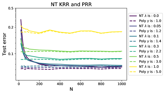
2.2 Comparing NT regression and polynomial regression

In the second experiment, we generated data from a linear model $y_{i}=\langle\text{\boldmath$x$}_{i},\text{\boldmath$\beta$}_{*}\rangle+\varepsilon_{i}$ . As before, $\text{\boldmath$x$}_{i}\sim\mathrm{Unif}(\mathbb{S}^{d-1}(\sqrt{d}))$ , $\varepsilon_{i}\sim{\mathcal{N}}(0,\sigma^{2}_{\varepsilon})$ , $\sigma_{\varepsilon}=0.5$ , and $\text{\boldmath$\beta$}_{*}$ is a fixed unit norm vector (randomly generated and then fixed throughout). In Figure 3, We fix $n=4000$ and $d=500$ , and vary the number of neurons \seqsplit $N\in\{10,20,\ldots,90,100,\ldots,1000\}$ . In Figure 4, we fix $N=800$ and $d=500$ , and vary the sample size \seqsplit $n\in\{100,200,\ldots,900,1000,1500,\ldots,4000\}$ . The results are averaged over $n_{\text{rep}}=10$ repetitions.

Notice that in all of these experiments $n\ll d^{2}$ . The theory developed below (see in particular Theorem 3.3 and Corollary 3.2) implies that the risk of NT ridge regression should be well approximated by the risk polynomial ridge regression, although with an inflated ridge parameter. For $n\ll d^{2}$ , the polynomial degree is $\ell=1$ . If $\lambda\geq 0$ denotes the regularization parameter in NT ridge regression, the equivalent regularization in polynomial regression is predicted to be

\gamma=\frac{\lambda+\mathrm{Var}(\sigma^{\prime})}{\big{\{}\mathbb{E}\big{[}\sigma^{\prime}(G)]\big{\}}^{2}},

(5)

where $G\sim\mathcal{N}(0,1)$ .

In Figures 3 and 4 we fit NT ridge regression (NT) and polynomial ridge regression of degree $\ell=1$ (Poly). We use different pairs of regularization parameters $\lambda$ (for NT) and $\gamma$ (for Poly), satisfying Eq. (5). We observe a close match between the risk of NT regression and polynomial, in agreement with the theory established below.

We also trained a two-layer neural network to fit this linear model. Under specific initialization of weights, the test error is well aligned with the one from NT KRR and polynomial ridge regression. Details can be found in the appendix.

3 Main results

3.1 Notations

For a positive integer, we denote by $[n]$ the set $\{1,2,\ldots,n\}$ . The $\ell_{2}$ norm of a vector $\text{\boldmath$u$}\in\mathbb{R}^{m}$ is denoted by $\|\text{\boldmath$u$}\|$ . We denote by $\mathbb{S}^{d-1}(r)=\{\text{\boldmath$u$}\in\mathbb{R}^{d}:\|\text{\boldmath$u$}\|=r\}$ the sphere of radius $r$ in $d$ dimensions (sometimes we simply write $\mathbb{S}^{d-1}:=\mathbb{S}^{d-1}(1)$ ).

Let $\mathrm{\bf A}\in\mathbb{R}^{n\times m}$ be a matrix. We use $\sigma_{j}(\mathrm{\bf A})$ to denote the $j$ -th largest singular value of $\mathrm{\bf A}$ , and we also denote $\sigma_{\max}(\mathrm{\bf A})=\sigma_{1}(\mathrm{\bf A})$ and $\sigma_{\min}(\mathrm{\bf A})=\sigma_{\min\{m,n\}}(\mathrm{\bf A})$ . If $\mathrm{\bf A}$ is a symmetric matrix, we use $\lambda_{j}(\mathrm{\bf A})$ to denote its $j$ -th largest eigenvalue. We denote by $\|\mathrm{\bf A}\|_{\mathrm{op}}=\max_{\text{\boldmath$u$}\in\mathbb{S}^{m-1}}\|\mathrm{\bf A}\text{\boldmath$u$}\|$ the operator norm, by $\|\mathrm{\bf A}\|_{\max}=\max_{i\in[n],j\in[m]}|A_{ij}|$ the maximum norm, by $\|\mathrm{\bf A}\|_{F}=\big{(}\sum_{i,j}A_{ij}^{2}\big{)}^{1/2}$ the Frobenius norm, and by $\|\mathrm{\bf A}\|_{*}=\sum_{j=1}^{\min\{n,m\}}\sigma_{j}(\mathrm{\bf A})$ the nuclear norm (where $\sigma_{j}$ is the $j$ -th singular value). If $\mathrm{\bf A}\in\mathbb{R}^{n\times n}$ is a square matrix, the trace of $\mathrm{\bf A}$ is denoted by $\mathrm{Tr}(\mathrm{\bf A})=\sum_{i\in[n]}A_{ii}$ . Positive semi-definite is abbreviated as p.s.d.

We will use $O_{d}(\cdot)$ and $o_{d}(\cdot)$ for the standard big- $O$ and small- $o$ notation, where $d$ is the asymptotic variable. We write $a_{d}=\Omega_{d}(b_{d})$ for scalars $a_{d},b_{d}$ if there exists $d_{0},C>0$ such that $a_{d}\geq Cb_{d}$ for $d>d_{0}$ . For random variables $\xi_{1}(d)$ and $\xi_{2}(d)$ , $\xi_{1}(d)=O_{d,\mathbb{P}}(\xi_{2}(d))$ if for any $\varepsilon$ , there exists $C_{\varepsilon}>0$ and $d_{\varepsilon}>0$ such that

\mathbb{P}\big{(}|\xi_{1}(d)/\xi_{2}(d)|>C_{\varepsilon}\big{)}\leq\varepsilon,\qquad\text{for all}~{}d>d_{\varepsilon}.

Similarly, $\xi_{1}(d)=o_{d,\mathbb{P}}(\xi_{2}(d))$ if $\xi_{1}(d)/\xi_{2}(d)$ converges to $0$ in probability. Occasionally, we use the notation $\widetilde{O}_{d,\mathbb{P}}(\cdot)$ and $\widetilde{o}_{d,\mathbb{P}}(\cdot)$ : we write $\xi_{1}(d)=\widetilde{O}_{d,\mathbb{P}}(\xi_{2}(d))$ if there exists a constant $C>0$ such that $\xi_{1}(d)=O_{d,\mathbb{P}}((\log d)^{C}\xi_{2}(d))$ , and similarly we write $\xi_{1}(d)=\widetilde{o}_{d,\mathbb{P}}(\xi_{2}(d))$ if there exists a constant $C>0$ such that $\xi_{1}(d)=o_{d,\mathbb{P}}((\log d)^{C}\xi_{2}(d))$ . We may drop the subscript $d$ if there is no confusion in a context.

For a nonnegative sequence $(a_{d})_{d\geq 1}$ , we write $a_{d}=\mathrm{poly}(d)$ if there exists a constant $C>0$ such that $a_{d}\leq Cd^{C}$ .

Throughout, we will use $C,C_{0},C_{1},C_{2},C_{3}$ to refer to constants that do not depend on $d$ . In particular, for notational convenience, the value of $C$ may change from line to line.

Most of our statement apply to settings in which $N,n,d$ all grow to $\infty$ , while satisfying certain conditions. Without loss of generality, one can thing that such sequences are indexed by $d$ , with $N,n$ functions of $d$ .

Recall that we say that $A_{N,n,d}$ happens with high probability (abbreviated as w.h.p.) if its probability tends to one as $N,n,d\to\infty$ (in whatever way is specified in the text). In certain proofs, we will say that an event $A_{N,n,d}$ happens with very high probability if for every $\beta>0$ , we have $\lim_{d\to\infty}d^{\beta}\mathbb{P}(A_{N,n,d}^{c})=0$ (again, we think of $N,n\to\infty$ when $d\to\infty$ in whatever way prescribed in the text).

3.2 Definitions and assumptions

Throughout, we assume $\text{\boldmath$x$}_{i}\sim_{\mathrm{i.i.d.}}\mathrm{Unif}(\mathbb{S}^{d-1}(\sqrt{d}))$ and $\text{\boldmath$w$}_{k}\sim_{\mathrm{i.i.d.}}\mathrm{Unif}(\mathbb{S}^{d-1})$ . To a vector of covariates $\text{\boldmath$x$}\in\mathbb{R}^{d}$ , the NT model associates a (random) features vector $\text{\boldmath$\Phi$}(\text{\boldmath$x$})$ as per Eq. (2). We denote by $\text{\boldmath$\Phi$}\in\mathbb{R}^{n\times(Nd)}$ the matrix whose $i$ -th row contains the feature vector of the $i$ -th sample, and by $\mathrm{\bf K}_{N}:=\text{\boldmath$\Phi$}\text{\boldmath$\Phi$}^{\top}$ the corresponding empirical kernel:

\text{\boldmath$\Phi$}=\left[\begin{matrix}\text{\boldmath$\Phi$}(\text{\boldmath$x$}_{1})^{\top}\\ \text{\boldmath$\Phi$}(\text{\boldmath$x$}_{2})^{\top}\\ \ldots\\ \text{\boldmath$\Phi$}(\text{\boldmath$x$}_{n})^{\top}\end{matrix}\right]\in\mathbb{R}^{n\times(Nd)},\;\;\;\;\;\;\mathrm{\bf K}_{N}:=\text{\boldmath$\Phi$}\text{\boldmath$\Phi$}^{\top}\in\mathbb{R}^{n\times n}\,.

The entries of the kernel matrix take the form

[\mathrm{\bf K}_{N}]_{ij}=\frac{1}{Nd}\sum_{k=1}^{N}\sigma^{\prime}(\langle\text{\boldmath$x$}_{i},\text{\boldmath$w$}_{k}\rangle)\sigma^{\prime}(\langle\text{\boldmath$x$}_{j},\text{\boldmath$w$}_{k}\rangle)\langle\text{\boldmath$x$}_{i},\text{\boldmath$x$}_{j}\rangle\,.

(6)

The infinite-width kernel matrix is given by

[\mathrm{\bf K}]_{ij}=\mathbb{E}_{\text{\boldmath$w$}}\big{[}\sigma^{\prime}(\langle\text{\boldmath$x$}_{i},\text{\boldmath$w$}\rangle)\sigma^{\prime}(\langle\text{\boldmath$x$}_{j},\text{\boldmath$w$}\rangle)\big{]}\frac{\langle\text{\boldmath$x$}_{i},\text{\boldmath$x$}_{j}\rangle}{d}.

(7)

In terms of the featurization map $\Phi$ , an NT function $f\in\mathcal{F}_{{\sf NT}}^{N}(\text{\boldmath$W$})$ reads

\displaystyle f(\text{\boldmath$x$};\text{\boldmath$a$})=\langle\text{\boldmath$a$},\text{\boldmath$\Phi$}(\text{\boldmath$x$})\rangle\,,

(8)

where $\text{\boldmath$a$}=(\text{\boldmath$a$}_{1},\dots\text{\boldmath$a$}_{N})^{\top}\in\mathbb{R}^{Nd}$ .

Assumption 3.1.

Given an arbitrary integer $\ell\geq 1$ , and a small constant $c_{0}>0$ , we assume that the following hold for a sufficiently large constant $C_{0}$ (depending on $c_{0}$ , $\ell$ , and on the activation $\sigma$ )

	$\displaystyle c_{0}d\leq n\leq\frac{d^{2}}{(\log d)^{C_{0}}},$	$\displaystyle\text{if}~{}\ell=1,$		(9)
	$\displaystyle d^{\ell}(\log d)^{C_{0}}\leq n\leq\frac{d^{\ell+1}}{(\log d)^{C_{0}}},$	$\displaystyle\text{if}~{}\ell>1.$		(10)

Throughout, we assume that the activation function $\sigma:\mathbb{R}\to\mathbb{R}$ satisfies the following condition. Note that commonly used activation functions, such as ReLU, sigmoid, tanh, leaky ReLU, satisfy this condition. Low-degree polynomials are excluded from this assumption. We denote by $\mu_{k}(\sigma^{\prime})$ the $k$ -th coefficient in the Hermite expansion of $\sigma^{\prime}$ ; see its definition in Section 6, especially Eqn. 39.

Assumption 3.2 (polynomial growth).

We assume that $\sigma$ is weakly differentiable with weak derivative $\sigma^{\prime}$ satisfying $|\sigma^{\prime}(x)|\leq B(1+|x|)^{B}$ for some finite constant $B>0$ , and that $\sum_{k\geq\ell}[\mu_{k}(\sigma^{\prime})]^{2}>0$ .

Note that this condition is extremely mild: it is satisfied by any activation function of practical use. The existence of the weak derivative $\sigma^{\prime}$ is needed for the NT model to make sense at all. The assumption of polynomial growth for $\sigma^{\prime}$ ensures that we can use harmonic analysis on the sphere to analyze its behavior. Finally the condition $\sum_{k\geq\ell}[\mu_{k}(\sigma^{\prime})]^{2}>0$ is satisfied if $\sigma$ is not a polynomial of degree $\ell$ .

3.3 Structure of the kernel matrix

Given points $\text{\boldmath$x$}_{1},\dots\text{\boldmath$x$}_{n}$ , $\Phi$ has full row rank, i.e. ${\rm rank}(\text{\boldmath$\Phi$})=n$ if and only if for any choice of the labels or responses $y_{1},\dots,y_{n}\in\mathbb{R}$ , there exists a function $f\in\mathcal{F}_{{\sf NT}}^{N}(\text{\boldmath$W$})$ interpolating those data, i.e. $y_{i}=f(\text{\boldmath$x$}_{i})$ for all $i\leq n$ . This of course requires $Nd\geq n$ . Our first result—which is a direct corollary of Theorem 3.1 that we present below—shows that this lower bound is roughly correct.

Corollary 3.1.

Assume $(\text{\boldmath$x$}_{i})_{i\leq n}\sim_{\mathrm{i.i.d.}}\mathrm{Unif}(\mathbb{S}^{d-1}(\sqrt{d}))$ , and $(\text{\boldmath$w$}_{k})_{k\leq N}\sim_{\mathrm{i.i.d.}}\mathrm{Unif}(\mathbb{S}^{d-1}(1))$ , and let $B,c_{0}>0$ , $\ell\in\mathbb{N}$ be fixed. Then, there exist constants $C_{0},C>0$ such that the following holds.

If Assumptions 3.1 and 3.2 hold with constant $\ell,c_{0},C_{0},B$ , and if $Nd/(\log(Nd))^{C}\geq n$ , then ${\rm rank}(\text{\boldmath$\Phi$})=n$ with high probability. In particular an NT interpolator exists with high probability for any choice of the responses $(y_{i})_{i\leq n}$ .

Remark 1.

Note that any NT model (1) can be approximated arbitrarily well by a two-layer neural network with $2N$ neurons. This can be seen by taking $\varepsilon\to 0$ in $f_{\varepsilon}(\text{\boldmath$x$})=\sum_{k=1}^{N}\frac{1}{\varepsilon}\big{\{}\sigma(\langle\text{\boldmath$w$}_{k},\text{\boldmath$x$}\rangle+\varepsilon\langle\text{\boldmath$a$}_{k},\text{\boldmath$x$}\rangle)-\sigma(\langle\text{\boldmath$w$}_{k},\text{\boldmath$x$}\rangle-\varepsilon\langle\text{\boldmath$a$}_{k},\text{\boldmath$x$}\rangle)\big{\}}$ . As a consequence, in the above setting, a $2N$ -neurons neural network can interpolate $n$ data points with arbitrarily small approximation error with high probability provided $Nd/(\log(Nd))^{C}\geq n$ .

To the best of our knowledge, this is the first result of this type for regression. The concurrent paper [Dan20] proves a similar memorization result for classification but exploits in a crucial way the fact that in classification it is sufficient to ensure $y_{i}f(\text{\boldmath$x$}_{i})>0$ . Regression is considered in [BELM20] but the number of required neurons depends on the interpolation accuracy.

While we stated the above as an independent result because of its interest, it is in fact an immediate corollary of a quantitative lower bound on the minimum eigenvalue of the kernel $\mathrm{\bf K}_{N}\in\mathbb{R}^{n\times n}$ , stated below. Given $g:\mathbb{R}\to\mathbb{R}$ , we let $\mu_{k}(g)=\mathbb{E}[g(G)h_{k}(G)]$ denote its $k$ -th Hermite coefficient (here $G\sim{\mathcal{N}}(0,1)$ , $\mathbb{E}[h_{k}(G)^{2}]=1$ ); see also Section 6, Eq. 39.

Theorem 3.1.

If Assumptions 3.1 and 3.2 hold with constant $\ell,c_{0},C_{0},B$ , and further $n\geq d+1$ and $Nd/(\log(Nd))^{C}\geq n$ , then, defining $v(\sigma):=\sum_{k\geq\ell}[\mu_{k}(\sigma^{\prime})]^{2}$ , we have

\displaystyle\lambda_{\min}(\mathrm{\bf K}_{N})=v(\sigma)+o_{d,\mathbb{P}}(1)\,.

(11)

If the assumption $n\geq d+1$ is replaced by $n\geq c_{0}d$ for a strictly positive constant $c_{0}$ , then $\lambda_{\min}(\mathrm{\bf K}_{N})\geq v(\sigma)-o_{d,\mathbb{P}}(1)$ .

Remark 2.

In the case $\ell=1$ , the eigenvalue lower bound $v(\sigma)$ is simply $v(\sigma)={\rm Var}(\sigma^{\prime}(G))=\mathbb{E}[\sigma^{\prime}(G)^{2}]-\{\mathbb{E}[\sigma^{\prime}(G)]\}^{2}$ where $G\sim{\mathcal{N}}(0,1)$ .

The only earlier result comparable to Theorem 3.1 was obtained in [SJL18] which, in a similar setting, proved that, with high probability, $\lambda_{\min}(\mathrm{\bf K}_{N})\geq c_{*}$ for a strictly positive constant $c_{*}$ , provided $N\geq 2d$ .

The proof of Theorem 3.1 is presented in Section 7. The key is to show that the NT kernel concentrates to the infinite-width kernel for large enough $N$ .

For any constant $\gamma>0$ , we define an event $\mathcal{A}_{\gamma}$ as follows.

\mathcal{A}_{\gamma}=\big{\{}\mathrm{\bf K}\succeq\gamma\mathrm{\bf I}_{n},~{}\|\text{\boldmath$X$}\|_{\mathrm{op}}\leq 2(\sqrt{n}+\sqrt{d})\big{\}}.

(12)

This event only involves $(\text{\boldmath$x$}_{i})_{i\leq n}$ (formally speaking, it lies in the sigma-algebra generated by $(\text{\boldmath$x$}_{i})_{i\leq n}$ ). We will show that, if $\gamma>0$ is a constant no larger than $v(\sigma)/2$ , then the event $\mathcal{A}_{\gamma}$ happens with very high probability under Assumption 3.2, provided $n\leq d^{\ell+1}/(\log d)^{C_{0}}$ . Below we will use $\mathbb{P}_{\text{\boldmath$w$}}$ to mean the probability over the randomness of $\text{\boldmath$w$}_{1},\ldots,\text{\boldmath$w$}_{N}$ (equivalently, conditional on $(\text{\boldmath$x$}_{i})_{i\leq n}$ ).

Theorem 3.2 (Kernel concentration).

Assume $(\text{\boldmath$x$}_{i})_{i\leq n}\sim_{\mathrm{i.i.d.}}\mathrm{Unif}(\mathbb{S}^{d-1}(\sqrt{d}))$ , and $(\text{\boldmath$w$}_{k})_{k\leq N}\sim_{\mathrm{i.i.d.}}\mathrm{Unif}(\mathbb{S}^{d-1}(1))$ . Let $\gamma=v(\sigma)/2$ . Then, there exist constants $C^{\prime},C_{0}>0$ such that the following holds. Under Assumption 3.2, the event $A_{\gamma}$ holds with very high probability, and on the event $A_{\gamma}$ , for any constant $\beta>0$ ,

d^{\beta}\cdot\mathbb{P}_{\text{\boldmath$w$}}\left(\big{\|}\mathrm{\bf K}^{-1/2}\mathrm{\bf K}_{N}\mathrm{\bf K}^{-1/2}-\mathrm{\bf I}_{n}\big{\|}_{\mathrm{op}}>\sqrt{\frac{(n+d)(\log(nNd))^{C^{\prime}}}{Nd}}+\frac{(n+d)(\log(nNd))^{C^{\prime}}}{Nd}\right)=o_{d}(1).

As a consequence, if $n\leq d^{\ell+1}/(\log d)^{C_{0}}$ (i.e. the upper bound in Assumption 3.1 holds), with the same $\ell$ as in Assumption 3.2, then with very high probability,

\big{\|}\mathrm{\bf K}^{-1/2}\mathrm{\bf K}_{N}\mathrm{\bf K}^{-1/2}-\mathrm{\bf I}_{n}\big{\|}_{\mathrm{op}}\leq\sqrt{\frac{(n+d)(\log(nNd))^{C^{\prime}}}{Nd}}+\frac{(n+d)(\log(nNd))^{C^{\prime}}}{Nd}.

(13)

When the right-hand side of (13) is $o_{d,\mathbb{P}}(1)$ , it is clear that the eigenvalues of $\mathrm{\bf K}_{N}$ are bounded from below, since

\big{\|}\mathrm{\bf K}^{-1/2}\mathrm{\bf K}_{N}\mathrm{\bf K}^{-1/2}-\mathrm{\bf I}_{n}\big{\|}_{\mathrm{op}}\leq\eta^{\prime}\quad\Longrightarrow\quad(1-\eta^{\prime})\mathrm{\bf K}\preceq\mathrm{\bf K}_{N}\preceq(1+\eta^{\prime})\mathrm{\bf K}.

(14)

If we further have $n\leq Nd/(\log(Nd))^{C}$ , $n\geq c_{0}d$ for $c_{0}>0$ and a sufficiently large constant $C$ , then we can take $\eta^{\prime}=(n(\log(Nd))^{C^{\prime}}/Nd)^{1/2}$ here.

Remark 3.

If $\sigma^{\prime}$ is not a polynomial, then $\mathcal{A}_{\gamma}$ holds with high probability as soon as $n\leq d^{C^{\prime\prime}}$ for some constant $C^{\prime\prime}$ . Hence, in this case, the stronger assumption $n\leq d^{\ell+1}/(\log d)^{C_{0}}$ is not needed for the second part of this theorem.

3.4 Test error

In order to study the generalization properties of the NT model, we consider a general regression model for the data distribution. Data $(\text{\boldmath$x$}_{1},y_{1}),\ldots,(\text{\boldmath$x$}_{n},y_{n})$ are i.i.d. with $\text{\boldmath$x$}_{i}\sim\mathrm{Unif}(\mathbb{S}^{d-1}(\sqrt{d}))$ and $y_{i}=f_{*}(\text{\boldmath$x$}_{i})+\varepsilon_{i}$ where $f_{*}\in L^{2}:=L^{2}(\mathbb{S}^{d-1}(\sqrt{d}),\tau_{d-1})$ . Here, $L^{2}(\mathbb{S}^{d-1}(\sqrt{d}),\tau_{d-1})$ is the space of functions on $\mathbb{S}^{d-1}(\sqrt{d})$ which are square integrable with respect to the uniform measure. In matrix notation, we let $\text{\boldmath$X$}\in\mathbb{R}^{n\times d}$ denote the matrix whose $i$ -th row is $\text{\boldmath$x$}_{i}$ , $\text{\boldmath$y$}:=(y_{i})_{i\leq n}$ , and $\text{\boldmath$f$}_{*}=(f_{*}(\text{\boldmath$x$}_{i}))_{i\leq n}$ . We then have

\text{\boldmath$y$}=\text{\boldmath$f$}_{*}+\text{\boldmath$\varepsilon$},\qquad\text{where}~{}\mathrm{Var}(\varepsilon_{i})=\sigma_{\varepsilon}^{2}.

(15)

The noise variables $\varepsilon_{1},\ldots,\varepsilon_{n}\sim_{\mathrm{i.i.d.}}\mathbb{P}_{\varepsilon}$ are assumed to have zero mean and finite second moment, i.e., $\sigma_{\varepsilon}^{2}=\mathbb{E}(\varepsilon_{1}^{2})$ .

We fit the coefficients $\text{\boldmath$a$}=(\text{\boldmath$a$}_{1},\dots,\text{\boldmath$a$}_{N})\in\mathbb{R}^{Nd}$ of the NT model using ridge regression. Namely

\displaystyle\widehat{\boldsymbol{a}}(\lambda):=\arg\min_{\text{\boldmath$a$}\in\mathbb{R}^{Nd}}\Big{\{}\sum_{i=1}^{n}(y_{i}-f(\text{\boldmath$x$}_{i};\text{\boldmath$a$})\big{)}^{2}+\lambda\|\text{\boldmath$a$}\|^{2}\Big{\}}\,.

(16)

where $f(\,\cdot\,;\text{\boldmath$a$})$ is defined as per Eq. (1). Explicitly, we have

\widehat{\boldsymbol{a}}(\lambda)=\text{\boldmath$\Phi$}^{\top}\big{(}\text{\boldmath$\Phi$}\text{\boldmath$\Phi$}^{\top}+\lambda\mathrm{\bf I}_{n})^{-1}\text{\boldmath$y$}.

(17)

We evaluate this approach on a new input $\text{\boldmath$x$}_{0}$ that has the same distribution as the training input. Our analysis covers the case $\lambda=0$ , in which case we obtain the minimum $\ell_{2}$ -norm interpolator.

The test error is defined as

\displaystyle R_{{\sf NT}}(f_{*};\lambda)=\mathbb{E}_{\text{\boldmath$x$}_{0}}\big{[}(f_{*}(\text{\boldmath$x$}_{0})-\langle\widehat{\boldsymbol{a}}(\lambda),\text{\boldmath$\Phi$}(\text{\boldmath$x$}_{0})\rangle)^{2}\big{]}\,.

(18)

We occasionally call this ‘generalization error’, with a slight abuse of terminology (sometimes this term is referred to the difference between test error and the train error $n^{-1}\sum_{i\leq n}(y_{i}-\langle\widehat{\boldsymbol{a}},\text{\boldmath$\Phi$}(\text{\boldmath$x$}_{i})\rangle)^{2}$ .)

Our main results on the generalization behavior of NT KRR establish its equivalence with simpler methods. Namely, we perform kernel ridge regression with the infinite-width kernel $\mathrm{\bf K}$ . Let $\gamma\geq 0$ be any ridge regularization parameter. The prediction function fitted by the data alongside its associated risk is given by

	$\displaystyle\widehat{f}_{{\sf KRR}}^{\gamma}(\text{\boldmath$x$})=\mathrm{\bf K}(\cdot,\text{\boldmath$x$})^{\top}(\gamma\mathrm{\bf I}_{n}+\mathrm{\bf K})^{-1}\text{\boldmath$y$},$
	$\displaystyle R_{{\sf KRR}}(f_{};\gamma):=\mathbb{E}_{\text{\boldmath$x$}_{0}}\big{[}(f_{}(\text{\boldmath$x$}_{0})-\widehat{f}_{{\sf KRR}}^{\gamma}(\text{\boldmath$x$}_{0}))^{2}\big{]}.$

We also define the polynomial ridge regression as follows. The infinite-width kernel $K$ can be decomposed uniquely in orthogonal polynomials as $K(\text{\boldmath$x$},\text{\boldmath$x$}^{\prime})=\sum_{k=0}^{\infty}\gamma_{k}Q_{k}^{(d)}(\langle\text{\boldmath$x$},\text{\boldmath$x$}^{\prime}\rangle)$ , where $Q_{k}^{(d)}(z)$ is the Gegenbauer polynomial of degree $k$ (see Lemma 1). We consider truncating the kernel function up to the degree- $\ell$ polynomials:

K^{p}(\text{\boldmath$x$},\text{\boldmath$x$}^{\prime})=\sum_{k=0}^{\ell}\gamma_{k}Q_{k}^{(d)}(\langle\text{\boldmath$x$},\text{\boldmath$x$}^{\prime}\rangle).

(19)

The superscript refers to the name “polynomial”. We also define

\mathrm{\bf K}^{p}=\big{(}K^{p}(\text{\boldmath$x$}_{i},\text{\boldmath$x$}_{j})\big{)}_{i,j\leq n},\qquad\mathrm{\bf K}^{p}(\cdot,\text{\boldmath$x$})=\big{(}K^{p}(\text{\boldmath$x$}_{i},\text{\boldmath$x$})\big{)}_{i\leq n}.

(20)

For example, in the case $\ell=1$ , we have equivalence $\mathrm{\bf K}^{p}=\gamma_{0}\mathrm{\bf 1}_{n}\mathrm{\bf 1}_{n}^{\top}+\frac{\gamma_{1}}{d}\text{\boldmath$X$}\text{\boldmath$X$}^{\top}$ (the kernel of linear regression with an intercept). The prediction function fitted by the data and its associated risk are

	$\displaystyle\widehat{f}_{{\sf PRR}}^{\gamma}(\text{\boldmath$x$})=\mathrm{\bf K}^{p}(\cdot,\text{\boldmath$x$})^{\top}(\gamma\mathrm{\bf I}_{n}+\mathrm{\bf K}^{p})^{-1}\text{\boldmath$y$},$
	$\displaystyle R_{{\sf PRR}}(f_{};\gamma):=\mathbb{E}_{\text{\boldmath$x$}_{0}}\big{[}(f_{}(\text{\boldmath$x$}_{0})-\widehat{f}_{{\sf PRR}}^{\gamma}(\text{\boldmath$x$}_{0}))^{2}\big{]}.$

Kernel ridge regression and polynomial ridge regression are well understood. Our next result establishes a relation between these risks: the neural tangent model behaves as the polynomial model, albeit with a different value of the regularization parameter.

Theorem 3.3.

Assume $(\text{\boldmath$x$}_{i})_{i\leq n}\sim_{\mathrm{i.i.d.}}\mathrm{Unif}(\mathbb{S}^{d-1}(\sqrt{d}))$ , and $(\text{\boldmath$w$}_{k})_{k\leq N}\sim_{\mathrm{i.i.d.}}\mathrm{Unif}(\mathbb{S}^{d-1}(1))$ . Recall $v(\sigma):=\sum_{k\geq\ell}[\mu_{k}(\sigma^{\prime})]^{2}$ and let $B,c_{0}>0$ , $\ell\in\mathbb{N}$ be fixed. Then, there exist constants $C_{0},C,C^{\prime}>0$ such that the following holds.

If Assumptions 3.1 and 3.2 hold with constants $B,c_{0},\ell$ , and $Nd/(\log(Nd))^{C}\geq n$ , then for any $\lambda\geq 0$ ,

	$\displaystyle R_{{\sf NT}}(f_{*};\lambda)$	$\displaystyle=R_{{\sf KRR}}(f_{*};\lambda)+O_{d,\mathbb{P}}\Big{(}\tau^{2}\sqrt{\frac{n(\log(Nd))^{C^{\prime}}}{Nd}}\Big{)}$
		$\displaystyle=R_{{\sf PRR}}(f_{*};\lambda+v(\sigma))+O_{d,\mathbb{P}}\Big{(}\tau^{2}\sqrt{\frac{n(\log(Nd))^{C^{\prime}}}{Nd}}\,+\tau^{2}\sqrt{\frac{n(\log n)^{C}}{d^{\ell+1}}}\Big{)},$

where $\tau^{2}:=\|f_{*}\|^{2}_{L^{2}}+\sigma^{2}_{\varepsilon}$ .

Example: $n\ll d^{2}$ .

Suppose Assumptions 3.1 and 3.2 hold with $\ell=1$ , i.e. $c_{0}d\leq n\leq d^{2}/(\log d)^{C_{0}}$ . In this case, Theorem 3.3 implies that NT regression can only fit the linear component in the target function $f_{*}(\text{\boldmath$x$})$ . In order to simplify our treatment, we assume that the target is linear: $f_{*}(\text{\boldmath$x$})=\langle\text{\boldmath$\beta$}_{*},\text{\boldmath$x$}\rangle$ .

Consider ridge regression with respect to the linear features, with regularization $\gamma\geq 0$ :

	$\displaystyle\widehat{\boldsymbol{\beta}}(\gamma)$	$\displaystyle:=\arg\min_{\text{\boldmath$\beta$}\in\mathbb{R}^{d}}\Big{\{}\frac{1}{d}\sum_{i=1}^{n}(y_{i}-\langle\text{\boldmath$\beta$},\text{\boldmath$x$}_{i}\rangle\big{)}^{2}+\gamma\\|\text{\boldmath$\beta$}\\|_{2}^{2}\Big{\}}\,,$		(21)
	$\displaystyle R_{\mbox{\tiny\rm lin}}(f_{*};\gamma)$	$\displaystyle:=\mathbb{E}_{\text{\boldmath$x$}_{0}}\big{[}(\langle\text{\boldmath$\beta$}_{*},\text{\boldmath$x$}_{0}\rangle-\langle\widehat{\boldsymbol{\beta}}(\gamma),\text{\boldmath$x$}_{0}\rangle)^{2}\big{]}\,.$		(22)

Note that $R_{\mbox{\tiny\rm lin}}(f_{*};\gamma)$ is essentially the same as $R_{{\sf PRR}}(f_{*};\lambda+v(\sigma))$ , with the minor difference that we are not fitting an intercept. The scaling factor $d^{-1}$ is specially chosen for comparison with NT KRR. Theorem 3.3 implies the following correspondence.

Corollary 3.2 (NT KRR for linear model).

Assume $(\text{\boldmath$x$}_{i})_{i\leq n}\sim_{\mathrm{i.i.d.}}\mathrm{Unif}(\mathbb{S}^{d-1}(\sqrt{d}))$ , $(\text{\boldmath$w$}_{k})_{k\leq N}\sim_{\mathrm{i.i.d.}}\mathrm{Unif}(\mathbb{S}^{d-1}(1))$ , and $\mathbb{E}(\varepsilon_{i}^{4})\leq C\sigma_{\varepsilon}^{4}$ . Denote $\tau^{2}=\|\text{\boldmath$\beta$}_{*}\|^{2}+\sigma_{\varepsilon}^{2}$ . Then, there exist constants $C_{0},C>0$ such that the following holds. Under Assumption 3.1 and 3.2 with $\ell=1$ and $Nd/(\log(Nd))^{C}\geq n$ ,

	$\displaystyle R_{{\sf NT}}(f_{*};\lambda)$	$\displaystyle=R_{\mbox{\tiny\rm lin}}(f_{*};\gamma_{\mbox{\tiny\rm eff}}(\lambda,\sigma))+O_{d,\mathbb{P}}\Big{(}\tau^{2}\sqrt{\frac{n(\log d)^{C}}{Nd}}+\frac{\tau^{2}}{\sqrt{d}}+\tau^{2}\sqrt{\frac{n(\log n)^{C}}{d^{2}}}\Big{)}\,,\qquad\text{where}$		(23)
	$\displaystyle\gamma_{\mbox{\tiny\rm eff}}(\lambda,\sigma)$	$\displaystyle:=\frac{\lambda+v(\sigma)}{\{\mathbb{E}[\sigma^{\prime}(G)]\}^{2}}.\,$		(24)

Further,

$\displaystyle R_{\mbox{\tiny\rm lin}}(f_{*};\gamma)$	$\displaystyle=\\|\text{\boldmath$\beta$}_{*}\\|^{2}_{2}\mathscrsfs{B}_{\mbox{\tiny\rm lin}}(\gamma)+\sigma_{\varepsilon}^{2}\mathscrsfs{V}_{\mbox{\tiny\rm lin}}(\gamma)+O_{d,\mathbb{P}}(\tau^{2}/\sqrt{d}),$	(25)
$\displaystyle\mathscrsfs{B}_{\mbox{\tiny\rm lin}}(\gamma)$	$\displaystyle:=\frac{\gamma^{2}}{d}\mathrm{Tr}\Big{(}\big{(}\gamma{\boldsymbol{I}}_{d}+\text{\boldmath$X$}^{{\sf T}}\text{\boldmath$X$}/d\big{)}^{-2}\Big{)},$	(26)
$\displaystyle\mathscrsfs{V}_{\mbox{\tiny\rm lin}}(\gamma)$	$\displaystyle:=\frac{1}{d^{2}}\mathrm{Tr}\Big{(}\text{\boldmath$X$}^{{\sf T}}\text{\boldmath$X$}\big{(}\gamma{\boldsymbol{I}}_{d}+\text{\boldmath$X$}^{{\sf T}}\text{\boldmath$X$}/d\big{)}^{-2}\Big{)}\,.$	(27)

Remark 4.

The error term $O_{d,\mathbb{P}}(\tau^{2}d^{-1/2})$ in (23) is due to the effect of the intercept. It is easy to derive the asymptotic formulas if $n/d\to\kappa\in(0,\infty)$ where $\kappa$ is a constant [HMRT19]:

	$\displaystyle\mathscrsfs{B}_{\mbox{\tiny\rm lin}}(\kappa,\gamma)$	$\displaystyle=\frac{1}{2}\left\{1-\kappa+\sqrt{(\kappa-1+\gamma)^{2}+4\gamma}-\frac{\gamma(1+\kappa+\gamma)}{\sqrt{(\kappa-1+\gamma)^{2}+4\gamma}}\right\}+o_{d,\mathbb{P}}(1)\,,$		(28)
	$\displaystyle\mathscrsfs{V}_{\mbox{\tiny\rm lin}}(\kappa,\gamma)$	$\displaystyle=\frac{1}{2}\left\{-1+\frac{\kappa+\gamma+1}{\sqrt{(\kappa-1+\gamma)^{2}+4\gamma}}\right\}+o_{d,\mathbb{P}}(1)\,.$		(29)

Here we emphasized the dependence on $\kappa$ . Also, as $\kappa\to\infty$ , $\mathscrsfs{B}_{\mbox{\tiny\rm lin}}(\kappa,\gamma)=\gamma^{2}\kappa^{-2}+O(\kappa^{-3})$ and $\mathscrsfs{V}_{\mbox{\tiny\rm lin}}(\kappa,\gamma)=\kappa^{-1}+O(\kappa^{-2})$ .

In particular, the ridgeless NT model at $\lambda=0$ corresponds to linear regression with regularization $\gamma=v(\sigma)/\{\mathbb{E}[\sigma^{\prime}(G)]\}^{2}$ . Note that the denominator in (24) is due to the different scaling for the linear term (cf. Eq. 19). Since $\mathscrsfs{B}_{\mbox{\tiny\rm lin}}(\kappa,\gamma)=O(d^{2}/n^{2})$ and $\mathscrsfs{V}_{\mbox{\tiny\rm lin}}(\kappa,\gamma)=O(d/n)$ from the formulas (28) and (29), we find that the error term of order $\sqrt{n/Nd}$ in Eq. (23) is negligible for $1\leq n/d\ll N^{1/3}$ . We leave to future work the problem of obtaining optimal bounds on the error term.

3.5 An upper bound on the memorization capacity

In the regression setting, naively counting degrees of freedom would imply that the memorization capacity of a two-layer network with $N$ neurons is at most given by the number of parameters, namely $N(d+1)$ . More careful consideration reveals that, as long as the data $\{(\text{\boldmath$x$}_{i},y_{i})\}_{i\leq n}$ are in generic positions $N=O(1)$ neurons are sufficient to achieve memorization within any fixed accuracy, using a ‘sawlike’ activation function.

These constructions are of course fragile and a non-trivial upper bound on the memorization capacity can be obtained if we constrain the weights. In this section, we prove such an upper bound. We state it for binary classification, but it is immediate to see that it implies an upper bound on regression which is of the same order.

To simplify the argument, we assume $(\text{\boldmath$x$}_{i})_{i\leq n}\sim_{\mathrm{i.i.d.}}\mathcal{N}(\mathrm{\bf 0},\mathrm{\bf I}_{d})$ (which is very close to the setting $(\text{\boldmath$x$}_{i})_{i\leq n}\sim_{\mathrm{i.i.d.}}\mathrm{Unif}(\mathbb{S}^{d-1}(\sqrt{d})$ ) and $y_{1},\ldots,y_{n}\sim_{\mathrm{i.i.d.}}\mathrm{Unif}(\{+1,-1\})$ . Consider a subset of two-layers neural networks, by constraining the magnitude of the parameters:

\mathcal{F}_{{\sf NN}}^{N,L}:=\Big{\{}f(\text{\boldmath$x$};\text{\boldmath$b$},\text{\boldmath$W$})=\sum_{k=1}^{N}b_{k}\sigma\big{(}\langle\text{\boldmath$w$}_{\ell},\text{\boldmath$x$}\rangle\big{)},\quad N^{-1/2}\|\text{\boldmath$b$}\|\leq L,\|\text{\boldmath$w$}_{k}\|\leq L,~{}\forall\,k\in[N]\Big{\}}.

To get binary outputs from $f(\text{\boldmath$x$})\in\mathbb{R}$ , we take the sign. In particular, the label predict on sample $\text{\boldmath$x$}_{i}$ is $\mathrm{sign}(f(\text{\boldmath$x$}_{i}))$ .

The value $y_{i}f(\text{\boldmath$x$}_{i})$ is referred to the margin for input $\text{\boldmath$x$}_{i}$ . In regression we require $y_{i}f(\text{\boldmath$x$}_{i})=y_{i}^{2}=1$ (the latter equality holds for $\{+1,-1\}$ labels), while in classification we ask for $yf(\text{\boldmath$x$}_{i})>0$ . The next result states that $Nd$ must be roughly of order $n$ in order for a neural network to fit a nontrivial fraction of data with $\delta$ margin.

Proposition 3.1.

Let Assumptions 3.1 and 3.2 hold, and further assume $(\text{\boldmath$x$}_{i})_{i\leq n}\sim_{\mathrm{i.i.d.}}{\mathcal{N}}(\mathrm{\bf 0},{\boldsymbol{I}}_{d})$ . Fix constants $\eta_{1},\eta_{2}>0$ , and let $L=L_{d}\geq 1$ , $\delta=\delta_{d}>0$ be general functions of $d$ . Then there exists a constant $C$ such that the following holds.

Assume that, with probability larger than $\eta_{1}$ , there exists a function $f\in\mathcal{F}_{{\sf NN}}^{N,L}$ such that

\frac{1}{n}\sum_{i=1}^{n}\mathrm{\bf 1}\{y_{i}f(\text{\boldmath$x$}_{i})>\delta\}\geq\frac{1+\eta_{2}}{2}.

(30)

(In words, $f$ achieves margin $\delta$ in at least a fraction $(1+\eta_{2})/2$ of the samples.)

Then we must have $n\leq C^{-1}Nd\log(Ld/\delta)$ .

If $L$ and $1/\delta$ are upper bounded by a polynomial of $d$ , then this result implies an upper bound on the network capacity of order $Nd\log d$ . This matches the interpolation and invertibility thresholds in Corollary 3.1, and Theorem 3.1 up to a logarithmic factor. The proof follows a discretization–approximation argument, which can be found in the appendix.

Remark 5.

Notice that the memorization capacity upper bound $C^{-1}Nd\log(Ld/\delta)$ tends to infinity when the margin vanishes $\delta\to 0$ . This is not an artifact of the proof. As mentioned above, if we allow for an arbitrarily small margin, it is possible to construct a ‘sawlike’ activation function $\sigma$ such that the corresponding network correctly classifies $n$ points with binary labels $y_{i}\in\{+1,-1\}$ despite $n\gg Nd$ . Note that our result is different from [YSJ19, BHLM19] in which the activation function is piecewise linear/polynomial.

Remark 6.

While we stated Proposition 3.1 for classification, it has obvious consequences for regression interpolation. Indeed, considering $y_{i}\in\{+1,-1\}$ , the interpolation constraint $f(\text{\boldmath$x$}_{i})=y_{i}$ implies $y_{i}f(\text{\boldmath$x$}_{i})\geq\delta_{0}=1$ .

4 Related work

As discussed in the introduction, we addressed three questions: Q1: What is the maximum number of training samples $n$ that a network of given width $N$ can interpolate (or memorize)? Q2: Can such an interpolator be found efficiently? Q3: What are the generalization properties of the interpolator? While questions Q1 and Q2 have some history (which we briefly review next), much less is known about Q3, which is our main goal in this paper.

In the context of binary classification, question Q1 was first studied by Tom Cover [Cov65], who considered the case of a simple perceptron network ( $N=1$ ) when the feature vectors $(\text{\boldmath$x$}_{i})_{i\leq n}$ are in a generic position, and the labels $y_{i}\in\{+1,-1\}$ are independent and uniformly random. He proved that this model can memorize $n$ training samples with high probability if $n\leq 2d(1-\varepsilon)$ , and cannot memorize them with high probability if $n\geq 2d(1+\varepsilon)$ . Following Cover, this maximum number of samples is sometimes referred to as the network capacity but, for greater clarity, we also use the expression network memorization capacity.

The case of two-layers network was studied by Baum [Bau88] who proved that, again for any set of points in general positions, the memorization capacity is at least $Nd$ . Upper bound of the same order were proved, among others, in [Sak92, Kow94]. Generalizations to multilayer networks were proven recently in [YSJ19, Ver20]. Can these networks be found efficiently? In the context of classification, the recent work of [Dan19] provides an efficient algorithm that can memorize all but a fraction $\varepsilon$ of the training samples in polynomial time, provided the $Nd\geq Cn/\varepsilon^{2}$ . For the case of Gaussian feature vectors, [Dan20] proves that exact memorization can be achieved efficiently provided $Nd\geq Cn(\log d)^{4}$ .

Here we are interested in achieving memorization in regression, which is more challenging than for classification. Indeed, in binary classification a function $f:\mathbb{R}^{d}\to\mathbb{R}$ memorizes the data if $y_{i}f(\text{\boldmath$x$}_{i})>0$ for all $i\leq n$ . On the other hand, in our setting, memorization amounts to $f(\text{\boldmath$x$}_{i})=y_{i}$ for all $i\leq n$ . The techniques developed for binary classification exploit in a crucial way the flexibility provided by the inequality constraint, which we cannot do here.

In concurrent work, [BELM20] studied the interpolation properties of two-layers networks. Generalizing the construction of Baum [Bau88], they show that, for $N\geq 4\lceil n/d\rceil$ there exists a two-layers ReLU network interpolating $n$ points in generic positions. This is however unlikely to be the network produced by gradient-based training. They also construct a model that interpolates the data with error $\varepsilon$ , provided $Nd\geq n\log(1/\varepsilon)$ . In contrast, we obtain exact interpolation provided $Nd\geq n(\log Nd)^{C}$ From a more fundamental point of view, our work does not only construct a network that memorizes the data, but also characterizes the eigenstructure of the kernel matrix. While our paper is under review, more papers on memorization are posted, including [VYS21, PLYS21] that study the effect of depth.

As discussed in the introduction, we focus here on the lazy or neural tangent regime in which weights change only slightly with respect to a random initialization [JGH18]. This regime attracted considerable attention over the last two years, although the focus has been so far on its implications for optimization, rather than on its statistical properties.

It was first shown in [DZPS18] that, for sufficiency overparametrized networks, and under suitable initializations, gradient-based training indeed converges to an interpolator that is well approximated by an NT model. The proof of [DZPS18] required (in the present context) $N\geq Cn^{6}/\lambda_{\min}(\mathrm{\bf K})^{4}$ , where $\mathrm{\bf K}$ is the infinite width kernel of Eq. (7). This bound was improved over the last two years [DZPS18, AZLS19, LXS⁺19, ZCZG20, OS20, LZB20, WCL20]. In particular, [OS20] prove that, for $Nd\geq Cn^{2}$ , gradient descent converges to an interpolator. The authors also point out the gap between this result and the natural lower bound $Nd\gtrsim n$ .

A key step in the analysis of gradient descent in the NT regime is to prove that the tangent feature map at the initialization (the matrix $\text{\boldmath$\Phi$}\in\mathbb{R}^{n\times Nd}$ ) or, equivalently, the associated kernel (i.e. the matrix $\mathrm{\bf K}_{N}=\text{\boldmath$\Phi$}\text{\boldmath$\Phi$}^{\top}$ ) is nonsingular. Our Theorem 3.1 establishes that this is the case for $Nd\geq n(\log d)^{C}$ . As discussed in Section 5, this implies convergence of gradient descent under the near-optimal condition $Nd\geq n(\log d)^{C}$ , under a suitable scaling of the weights [COB19]. More generally, our characterization of the eigenstructure of $\mathrm{\bf K}_{N}$ is a foundational step towards a sharper analysis of the gradient descent dynamics.

As mentioned several times, our main contribution is a characterization of the test error of minimum norm regression in the NT model (1). We are not aware of any comparable results.

Upper bounds on the generalization error of neural networks based on NT theory were proved, among others, in [ADH⁺19, AZLL19, CG19, JT19, CCZG19, NCS19]. These works assume a more general data distribution than ours. However their objectives are of very different nature from ours. We characterize the test error of interpolators, while most of these works do not consider interpolators. Our main result is a sharp characterization of the difference between test error of NT regression (with a finite number of neurons $N$ ) and kernel ridge regression (corresponding to $N=\infty$ ), and between this and polynomial regression. None of the earlier work is sharp enough to provide to control these quantities. More in detail:

•

The upper bound of [ADH⁺19] applies to interpolators but controls the generalization error by $(\langle\text{\boldmath$y$},\mathrm{\bf K}^{-1}\text{\boldmath$y$}\rangle/n)^{1/2}$ which, in the setting studied in the present paper, is a quantity of order one.
•

The upper bounds of [AZLL19, CG19] do not apply to interpolators since SGD is run in a one-pass fashion. Further they require large overparametrization, namely $N\gtrsim n^{7}$ in [CG19] and $N$ depending on the generalization error in [AZLL19]. Finally, they bound generalization error rather than test error, and do not bound the difference between NT regression and kernel ridge regression.
•

The upper bounds of [JT19, CCZG19, NCS19] apply to classification and require a large margin condition. As before, these papers do not bound the difference between NT regression and kernel ridge regression.

Results similar to ours were recently obtained in the context of simpler random features models in [HMRT19, GMMM21, MM21, MRSY19, GMMM20, MMM21]. The models studied in these works corresponds to a two-layer network in which the first layer is random and the second is trained. Their analysis is simpler because the featurization map has independent coordinates.

Finally, the closest line of work in the literature is one that characterizes the risk of KRR and KRR interpolators in high dimensions [Bac17, LR20, GMMM21, BM19, LRZ20, MMM21]. It is easy to see that the infinite width limit ( $N\to\infty$ at $n,d$ fixed), NT regression converges to kernel ridge(–less) regression (KRR) with the rotationally invariant kernel $\mathrm{\bf K}$ . Our work address the natural open question in these studies: how large $N$ should be for NT regression to approximate KRR with respect to the limit kernel? By considering scalings in which $N,n,d$ are all large and polynomially related, we showed that NT performs KRR already when $Nd/(\log Nd)^{C}\geq n$ .

5 Connections with gradient descent training of neural networks

In this section we discuss in greater detail the relation between the NT model (1) studied in the rest of the paper, and fully nonlinear two-layer neural networks. For clarity, we will adopt the following notation for the NT model:

\displaystyle f_{{\sf NT}}(\text{\boldmath$x$};\text{\boldmath$a$},\text{\boldmath$W$}):=\frac{1}{\sqrt{N}}\sum_{k=1}^{N}\langle\text{\boldmath$a$}_{k},\text{\boldmath$x$}\rangle\sigma^{\prime}(\langle\text{\boldmath$w$}_{k},\text{\boldmath$x$}\rangle)\,.

(31)

We changed the normalization purely for aesthetic reasons: since the model is linear, this has no impact on the min-norm interpolant. We will compare it to the following neural network

\displaystyle f_{{\sf NN}}(\text{\boldmath$x$};\widetilde{\text{\boldmath$W$}}):=\frac{\alpha}{\sqrt{N}}\sum_{k=1}^{2N}b_{k}\sigma(\langle\widetilde{\text{\boldmath$w$}}_{k},\text{\boldmath$x$}\rangle),~{}~{}b_{1}=\dots=b_{N}=+1\,,\;b_{N+1}=\dots=b_{2N}=-1\,.

(32)

Note that the network has $2N$ hidden units and the second layer weights $b_{k}$ are fixed. We train the first-layer weights using gradient flow with respect to the empirical risk

\displaystyle\frac{{\rm d}\phantom{t}}{{\rm d}t}\widetilde{\text{\boldmath$W$}}^{t}=-\nabla_{\text{\boldmath$W$}}\widehat{R}_{n}(\widetilde{\text{\boldmath$W$}}^{t})\,,\;\;\;\;\text{where}~{}~{}\widehat{R}_{n}(\widetilde{\text{\boldmath$W$}}):=\frac{1}{n}\sum_{i=1}^{n}\big{(}y_{i}-f_{{\sf NN}}(\text{\boldmath$x$};\widetilde{\text{\boldmath$W$}})\big{)}^{2}\,.

(33)

We use the following initialization:

\displaystyle\widetilde{\text{\boldmath$w$}}^{0}_{k}=\text{\boldmath$w$}^{0}_{N+k}=\widetilde{\text{\boldmath$w$}}_{k}\,\;\;\;\forall k\leq N\,.

(34)

Under this initialization, the network evaluates to $0$ at $t=0$ . Namely, $f_{{\sf NN}}(\text{\boldmath$x$};\widetilde{\text{\boldmath$W$}}^{0})=0$ for all $\text{\boldmath$x$}\in\mathbb{R}^{d}$ . Let us also emphasize that the weights $\text{\boldmath$w$}_{k}$ in the NT model (31) are chosen to match the ones in the initialization (34): in particular, we can take $(\text{\boldmath$w$}_{k})_{k\leq N}\sim_{\mathrm{i.i.d.}}\mathrm{Unif}(\mathbb{S}^{d-1}(1))$ to recover the neural tangent model treated in the rest of the paper. This symmetrization is a standard technique [COB19]: it simplifies the analysis because it implies $f_{{\sf NN}}(\text{\boldmath$x$};\widetilde{\text{\boldmath$W$}}^{0})=0$ . We refer Remark 7 $(ii)$ for explanations.

The next theorem is a slight modification of [BMR21, Theorem 5.4] which in turn is a refined version of the analysis of [COB19, OS20].

Theorem 5.1.

Consider the two-layer neural network of (32) trained with gradient flow from initialization (34), and the associated NT model of Eq. (31). Assume $(\text{\boldmath$w$}_{k})_{k\leq N}\sim_{\mathrm{i.i.d.}}\mathrm{Unif}(\mathbb{S}^{d-1}(1))$ , the activation function to have bounded second derivative $\sup_{t\in\mathbb{R}}|\sigma^{\prime\prime}(t)|\leq C$ , and its Hermite coefficients to satisfy $\mu_{k}(\sigma)\neq 0$ for all $k\leq\ell_{0}$ for some constant $\ell_{0}$ . Further assume $\{(\text{\boldmath$x$}_{i},y_{i})\}_{i\leq n}$ are i.i.d. with $\text{\boldmath$x$}_{i}\sim\mathrm{Unif}(\mathbb{S}^{d-1}(\sqrt{d}))$ and $y_{i}$ to be $C$ -subgaussian.

Then there exist constants $C_{i}$ , depending uniquely on $\sigma,\ell_{0}$ , such that if $d\leq n\leq d^{\ell_{0}}/(\log d)^{C_{0}}$ , as well as

\displaystyle n\leq\frac{Nd}{(\log Nd)^{C_{0}}}\;\;\;\mbox{ and }\;\;\;\alpha\geq C_{0}\sqrt{\frac{n^{2}}{Nd}}\,,

(35)

then, with probability at least $1-2\exp\{-n/C_{0}\}$ , the following holds.

Gradient flow converges exponentially fast to a global minimizer. Specifically, letting $\lambda_{*}=\lambda_{\min}(\mathrm{\bf K}_{N})\alpha^{2}d/(4n)$ , we have, for all $t\geq 0$ ,

\displaystyle\widehat{R}_{n}(\widetilde{\text{\boldmath$W$}}^{t})\leq\widehat{R}_{n}(\widetilde{\text{\boldmath$W$}}^{0})\,e^{-\lambda_{*}t}\,.

(36)

In particular the rate is lower bounded as $\lambda_{*}\geq C_{1}\alpha^{2}d/n$ by Theorem 3.1.

The model learned by gradient flow and min- $\ell_{2}$ norm interpolant are similar on test data. Namely, writing $f_{{\sf NN}}(\widetilde{\text{\boldmath$W$}}):=f_{{\sf NN}}(\,\cdot\,;\widetilde{\text{\boldmath$W$}})$ and $f_{{\sf NT}}(\text{\boldmath$W$}):=f_{{\sf NT}}(\,\cdot\,;\text{\boldmath$a$},\text{\boldmath$W$})$ , we have

\displaystyle\limsup_{t\to\infty}\|f_{{\sf NN}}(\widetilde{\text{\boldmath$W$}}^{t})-f_{{\sf NT}}(\widehat{\text{\boldmath$a$}},\text{\boldmath$W$})\|_{L^{2}(\mathbb{P})}\leq C_{1}\left\{\frac{1}{\alpha}\sqrt{\frac{n^{2}}{Nd}}+\frac{1}{\alpha^{2}}\sqrt{\frac{n^{5}}{Nd^{4}}}\right\}\,,

(37)

for $\widehat{\text{\boldmath$a$}}$ the coefficients of the min- $\ell_{2}$ norm interpolant of Eq. (3).

Notice that any generic activation function satisfies the condition $\mu_{k}(\sigma)\neq 0$ for all $k\leq\ell_{0}$ . For instance a sigmoid or smoothed ReLU with a generic offset satisfy the assumptions of this theorem.

The only difference with respect to [BMR21, Theorem 5.4] is that we assume $\text{\boldmath$x$}_{i}\sim\mathrm{Unif}(\mathbb{S}^{d-1}(\sqrt{d}))$ while [BMR21] assumes $\text{\boldmath$x$}_{i}\sim{\mathcal{N}}(\mathrm{\bf 0},{\boldsymbol{I}}_{d})$ . However, it is immediate to adapt the proof of [BMR21], in particular using Theorem 3.1 to control the minimum eigenvalue of the kernel at initialization.

Note that Theorem 5.1 requires the activation function $\sigma$ to be smoother than other results in this paper (it requires a bounded second derivative). This assumption is used to bound the Lipschitz constant of the Jacobian $\mathrm{\bf D}_{\text{\boldmath$W$}}f_{{\sf NN}}(\text{\boldmath$x$};\text{\boldmath$W$})$ uniformly over $W$ . We expect that a more careful analysis could avoid assuming such a strong uniform bound.

The difference in test errors between the neural network (32) trained via gradient flow and the min-norm NT interpolant studied in this paper can be bounded using Eq. (37) by triangular inequality. Also, while we focus for simplicity on gradient flow, similar results hold for gradient descent with small enough step size.

A few remarks are in order.

Remark 7.

Even among two-layer fully connected neural networks, model (32) presents some simplifications:

(i)

Second-layer weights are not trained and fixed to $b_{j}\in\{+1,-1\}$ . If second-layer weights are trained, the NT model (31) needs to be modified as follows

\displaystyle f_{{\sf NT}}(\text{\boldmath$x$};\text{\boldmath$a$},\text{\boldmath$W$}):=\frac{1}{\sqrt{N}}\sum_{i=1}^{N}\langle\text{\boldmath$a$}_{i},\text{\boldmath$x$}\rangle\sigma^{\prime}(\langle\text{\boldmath$w$}_{i},\text{\boldmath$x$}\rangle)+\frac{1}{\sqrt{N}}\sum_{i=1}^{N}\widetilde{a_{i}}\sigma(\langle\text{\boldmath$w$}_{i},\text{\boldmath$x$}\rangle)\,.

(38)

The new model has $N(d+1)$ parameters $\text{\boldmath$a$}=(\text{\boldmath$a$}_{1},\dots,\text{\boldmath$a$}_{N};\widetilde{a}_{1},\dots,\widetilde{a}_{N})$ . Notice that, for large dimension, the additional number of parameters is negligible. Indeed, going through the proofs reveals that our analysis can be extended to this case at the price of additional notational burden, but without changing the results.

We also point out that the model in which only second layer weights are trained, i.e. we set $\text{\boldmath$a$}_{i}=0$ in Eq. (38), has been studied in detail in [GMMM21, MMM21]. These papers support the above parameter-counting heuristics.

$(ii)$

The specific initialization (34) is chosen so that $f_{{\sf NN}}(\text{\boldmath$x$};\widetilde{\text{\boldmath$W$}}^{0})=0$ identically. If this initialization was modified (for instance by taking independent $(\widetilde{\text{\boldmath$w$}}_{k})_{k\leq 2N}$ ) two main elements would change in the analysis. First, the target model $f_{*}(\text{\boldmath$x$})$ should be replaced by the difference between target and initialization $f_{*}(\text{\boldmath$x$})-f_{{\sf NN}}(\text{\boldmath$x$};\widetilde{\text{\boldmath$W$}}^{0})$ . Second, and more importantly, the approximation results in Theorem 5.1 become weaker: we refer to [BMR21] for a comparison.

Remark 8.

Within the setting of Theorem 5.1 (in particular $y_{i}$ being $C$ -subgaussian), the null risk $\|f_{*}\|^{2}_{L^{2}}$ is of order one, and therefore we should compare the right-hand side of Eq. (37) with $\|f_{*}\|_{L^{2}}=\Theta(1)$ . We can point at two specific regimes in which this upper bound guarantees that $\|f_{{\sf NN}}(\widetilde{\text{\boldmath$W$}}^{\infty})-f_{{\sf NT}}(\widehat{\text{\boldmath$a$}},\text{\boldmath$W$})\|_{L^{2}}\ll\|f_{*}\|_{L^{2}}$ :

$(i)$

First letting $\alpha$ grow, the this upper bound vanishes. More precisely, it becomes much smaller than one provided $\alpha\gg(n^{2}/Nd)^{1/2}\vee(n^{5}/Nd^{4})^{1/4}$ . By training the two-layer neural network with a large scaling parameter $\alpha$ , we obtain a model that is well approximated by the NT model as soon as the overparametrization condition $n\leq Nd/(\log Nd)^{C}$ is satisfied.

This role of scaling in the network parameters, and its generality were first pointed out in [COB19]. It implies that the theory developed in this always applied to nonlinear neural networks under a certain specific initialization and training scheme.
$(ii)$

A standard initialization rule suggests to take $\alpha=\Theta(1)$ . In this case, the right-hand side of Eq. (37) becomes small for wide enough networks, namely $Nd\gg n^{2}\vee(n^{5}/d^{4})$ . This condition is stronger than the overparametrization condition under which we carried our analysis of the NT model.

This means that, for $\alpha=\Theta(1)$ and $n(\log n)^{C}\ll Nd\lesssim n^{2}\vee(n^{5}/d^{4})$ , we can apply our analysis to neural tangent models but not to actual neural networks. On the other hand, the condition $Nd\gg n^{2}\vee(n^{5}/d^{4})$ in Theorem 5.1 is likely to be a proof artifact, and we expect that it will be improved in the future. In fact we believe that the refined characterization of the NT model in the present paper is a foundational step towards such improvements.

Remark 9.

Theorem 5.1 relates the large-time limit of GD trained neural networks to the minimum $\ell_{2}$ -norm NT interpolators, corresponding to the case $\lambda=0$ of Eq. (17). The review paper [BMR21] proves a similar bound relating the NN and NT models, trained via gradient descent, at all times $t$ . Our main result, Theorem 3.3 characterizes the test error of NT regression with general $\lambda\geq 0$ . Going through the proof [BMR21, Theorem 5.4], it can be seen that a non-vanishing $\lambda>0$ corresponds to regularizing GD training of the two-layer neural network by the penalty $\|\text{\boldmath$W$}-\text{\boldmath$W$}^{0}\|_{F}^{2}=\sum_{\ell\leq N}\|\text{\boldmath$w$}_{\ell}-\text{\boldmath$w$}_{\ell}^{0}\|_{2}^{2}$ .

6 Technical background

This subsection provides a very short introduction to Hermite polynomials and Gegenbauer polynomials. More background information can be found in [AH12, CC14, GMMM21] for example. Let $\rho$ be standard Gaussian measure on $\mathbb{R}$ , namely $\rho(dx)=(2\pi)^{-1/2}e^{-x^{2}/2}\;dx$ . The space $L^{2}(\mathbb{R},\rho)$ is a Hilbert space with the inner product $\langle f,g\rangle_{L^{2}(\mathbb{R},\rho)}=\mathbb{E}_{G\sim\rho}[f(G)g(G)]$ .

The Hermite polynomials form a complete orthogonal basis of $L^{2}(\mathbb{R},\rho)$ . Throughout this paper, we will use normalized Hermite polynomials $\{h_{k}\}_{k\geq 0}$ :

\mathbb{E}\big{[}h_{k}(G)h_{j}(G)\big{]}=\delta_{kj}.

where $\delta_{kj}$ is Kronecker delta, namely $\delta_{kj}=0$ if $k\neq j$ and $\delta_{kj}=1$ if $k=j$ . For example, the first four Hermite polynomials are given by $h_{0}(x)=1,h_{1}(x)=x,h_{2}(x)=\frac{1}{\sqrt{2}}(x^{2}-1)$ and $h_{3}(x)=\frac{1}{\sqrt{6}}(x^{3}-3x)$ . For any function $f\in L^{2}(\mathbb{R},\rho)$ , we have decomposition

f=\sum_{k=0}^{\infty}\langle f,h_{k}\rangle_{L^{2}(\mathbb{R},\rho)}\;h_{k}.

In particular, if $\sigma^{\prime}\in L^{2}(\mathbb{R},\rho)$ , we denote $\mu_{k}=\langle\sigma^{\prime},h_{k}\rangle_{L^{2}(\mathbb{R},\rho)}$ and have

\sigma^{\prime}=\sum_{k=0}^{\infty}\mu_{k}h_{k}.

(39)

Let $\tau_{d-1}$ be the uniform probability measure on $\mathbb{S}^{d-1}(\sqrt{d})$ , $\widetilde{\tau}_{d-1}^{1}$ be the probability measure of $\sqrt{d}\,\langle\text{\boldmath$x$},\text{\boldmath$e$}_{1}\rangle$ where $\text{\boldmath$x$}\sim\tau_{d-1}$ , and $\tau_{d-1}^{1}$ be the probability measure of $\langle\text{\boldmath$x$},\text{\boldmath$e$}_{1}\rangle$ . The Gegenbauer polynomials $(Q_{k}^{(d)})_{k=0}^{\infty}$ form a basis of $L^{2}([-d,d],\widetilde{\tau}_{d-1}^{1})$ (for simplicity, we may write it as $L^{2}$ unless confusion arises) where $Q_{k}^{(d)}$ is a polynomial of degree of $k$ and the they satisfy the normalization

\langle Q_{k}^{(d)},Q_{j}^{(d)}\rangle_{L^{2}}=\frac{1}{B(d,k)}\delta_{jk}

where $B(d,k)$ is a dimension parameter that is monotonically increasing in $k$ and satisfies $B(d,k)=(1+o_{d}(1))d^{k}/k!$ . This normalization guarantees $Q_{k}^{(d)}(d)=1$ . The following are some properties of Gegenbauer polynomials we will use.

(a)

For $\text{\boldmath$x$},\text{\boldmath$y$}\in\mathbb{S}^{d-1}(\sqrt{d})$ ,

\big{\langle}Q_{k}^{(d)}(\langle\text{\boldmath$x$},\cdot\rangle),Q_{j}^{(d)}(\langle\text{\boldmath$y$},\cdot\rangle)\big{\rangle}_{L^{2}(\mathbb{S}^{d-1}(\sqrt{d}),\tau_{d-1})}=\frac{1}{B(d,k)}\delta_{jk}Q_{k}^{(d)}(\langle\text{\boldmath$x$},\text{\boldmath$y$}\rangle).

(40)

(b)

For $\text{\boldmath$x$},\text{\boldmath$y$}\in\mathbb{S}^{d-1}(\sqrt{d})$ ,

Q_{k}^{(d)}(\langle\text{\boldmath$x$},\text{\boldmath$y$}\rangle)=\frac{1}{B(d,k)}\sum_{i=1}^{B(d,k)}Y_{ki}^{(d)}(\text{\boldmath$x$})Y_{ki}^{(d)}(\text{\boldmath$y$}),

(41)

where $Y_{k,1}^{(d)},\ldots,Y_{k,B(d,k)}^{(d)}$ are normalized spherical harmonics of degree $k$ ; more precisely, each $Y_{k,i}^{(d)}$ is a polynomial of degree $k$ and they satisfy

\langle Y_{k,i}^{(d)},Y_{m,j}^{(d)}\rangle_{L^{2}(\mathbb{S}^{d-1}(\sqrt{d}),\tau_{d-1})}=\delta_{km}\delta_{ij}.

(42)

$(c)$

Recurrence formula. For $t\in[-d,d]$ ,

$\frac{t}{d}Q_{k}^{(d)}(t)=\frac{k}{2k+d-2}Q_{k-1}^{(d)}(t)+\frac{k+d-2}{2k+d-2}Q_{k+1}^{(d)}(t).$ (43)

(d)

Connection to Hermite polynomials. If $f\in L^{2}(\mathbb{R},\rho)\cap L^{2}([-\sqrt{d},\sqrt{d}],\tau_{d-1}^{1})$ , then

\mu_{k}(f)=\lim_{d\to\infty}\sqrt{B(d,k)}\,\langle f,Q_{k}^{(d)}(\sqrt{d}\,\cdot)\rangle_{L^{2}([-\sqrt{d},\sqrt{d}],\tau_{d-1}^{1})}.

(44)

Note that point $(b)$ and the Cauchy-Schwarz inequality implies $\max_{|t|\leq d}|Q_{k}^{(d)}(t)|\leq 1$ . If the function $\sigma^{\prime}$ satisfies $\sigma^{\prime}\in L^{2}([-\sqrt{d},\sqrt{d}],\tau_{d-1}^{1})$ , then we can decompose $\sigma^{\prime}$ using Gegenbauer polynomials:

	$\displaystyle\sigma^{\prime}(x)=\sum_{k=0}^{\infty}\lambda_{d,k}(\sigma^{\prime})B(d,k)Q_{k}^{(d)}(\sqrt{d}\,x),\qquad\text{where}$		(45)
	$\displaystyle\lambda_{d,k}(\sigma^{\prime}):=\langle\sigma^{\prime},Q_{k}^{(d)}(\sqrt{d}\,\cdot)\big{\rangle}_{L^{2}([-\sqrt{d},\sqrt{d}],\tau_{d-1}^{1})}.$		(46)

We also have $\|\sigma^{\prime}\|_{L^{2}([-\sqrt{d},\sqrt{d}],\tau_{d-1}^{1})}^{2}=\sum_{k=0}^{\infty}B(d,k)[\lambda_{d,k}(\sigma^{\prime})]^{2}$ . We sometimes drop the subscript $k$ if no confusion arises.

7 Kernel invertibility and concentration: Proof of Theorems 3.1 and 3.2

Our analysis starts with a study of the infinite-width kernel $\mathrm{\bf K}$ . In our setting, we will show that $\mathrm{\bf K}$ is essentially a regularized low-degree polynomial kernel plus a small ‘noise’. Such a decomposition will play an essential role in our analysis of the generalization error.

To ease notations, we will henceforth write the target function $f_{*}$ simply as $f$ .

7.1 Infinite-width kernel decomposition

Recall that we denote by $(Q_{k}^{(d)})_{k\geq 0}$ the Gegenbauer polynomials in $d$ dimensions, and denote by $(Y_{kt})_{t\leq B(d,k)}$ the normalized spherical harmonics of degree $k$ in $d$ dimensions. We denote by $\text{\boldmath$\Psi$}_{=k}\in\mathbb{R}^{n\times B(d,k)}$ the degree- $k$ spherical harmonics evaluated at $n$ data points, and denote by $\text{\boldmath$\Psi$}_{\leq k}$ the concatenation of these matrices of degree no larger than $k$ ; namely,

\text{\boldmath$\Psi$}_{\leq\ell}=\big{[}\text{\boldmath$\Psi$}_{=0},\ldots,\text{\boldmath$\Psi$}_{=\ell}\big{]},\qquad\text{where}~{}\text{\boldmath$\Psi$}_{=k}=\big{(}Y_{kt}(\text{\boldmath$x$}_{i})\big{)}_{i\leq n,t\leq B(d,k)}.

Lemma 1 (Harmonic decomposition of the infinite-width kernel).

The kernel $K$ can be decomposed as

\displaystyle K(\text{\boldmath$x$},\text{\boldmath$x$}^{\prime})=\sum_{k=0}^{\infty}\gamma_{k}Q_{k}^{(d)}(\langle\text{\boldmath$x$},\text{\boldmath$x$}^{\prime}\rangle)\,,

(47)

with coefficients:

\displaystyle\gamma_{0}=\big{[}\lambda_{1}(\sigma^{\prime})\big{]}^{2},\qquad\gamma_{k}=\frac{k+1}{2k+d}B(d,k+1)\big{[}\lambda_{k+1}(\sigma^{\prime})\big{]}^{2}+\frac{k+d-3}{2k+d-4}B(d,k-1)\big{[}\lambda_{k-1}(\sigma^{\prime})\big{]}^{2},

(48)

where the coefficients $\lambda_{k}=\lambda_{d,k}$ are defined in (46). The convergence in (47) takes place in any of the following interpretations: $(i)$ As functions in $L^{2}(\mathbb{S}^{d-1}(\sqrt{d})\times\mathbb{S}^{d-1}(\sqrt{d}),\tau_{d-1}\otimes\tau_{d-1})$ ; $(ii)$ Pointwise, for every $\text{\boldmath$x$},\text{\boldmath$x$}^{\prime}\in\mathbb{S}^{d-1}(\sqrt{d})\times\mathbb{S}^{d-1}(\sqrt{d})$ ; $(iii)$ In operator norm as integral operators $L^{2}(\mathbb{S}^{d-1}(\sqrt{d}),\tau_{d-1})\to L^{2}(\mathbb{S}^{d-1}(\sqrt{d}),\tau_{d-1})$ .

Finally, $\gamma_{0}=o_{d}(1)$ and for $k\geq 1$ we have $\gamma_{k}=\mu_{k-1}^{2}+o_{d}(1)$ , where we recall that $\mu_{k}$ is the $k$ -th coefficient in the Hermite expansion of $\sigma^{\prime}$ .

The use of spherical harmonics and Gegenbauer polynomials to study inner product kernels on the sphere (the $N=\infty$ case) is standard since the classical work of Schoenberg [Sch42]. Several recent papers in machine learning use these tools [Bac17, BM19, GMMM21]. On the other hand, quantitative properties when both the sample size $n$ and the dimension $d$ are large are much less studied [GMMM21]. The finite width $N$ case is even more challenging since the kernel is no longer of inner-product type.

Proof.

Recall the Gegenbauer decomposition of $\sigma^{\prime}$ in (45), implying that the following holds in $L^{2}(\mathbb{S}^{d-1})$ (we omit indicating the measure when this is uniform). For any fixed $\text{\boldmath$x$}\in\mathbb{S}^{d-1}(\sqrt{d})$ (and writing $\lambda_{k}(\sigma^{\prime}):=\lambda_{d,k}(\sigma^{\prime})$ ):

\displaystyle\sigma^{\prime}(\langle\text{\boldmath$x$},\,\cdot\,\rangle)=\sum_{k=0}^{\infty}\lambda_{k}(\sigma^{\prime})B(d,k)Q_{k}^{(d)}(\sqrt{d}\,\langle\text{\boldmath$x$},\,\cdot\,\rangle)\,.

We thus obtain, for fixed $x$ , $\text{\boldmath$x$}^{\prime}$ :

	$\displaystyle\mathbb{E}_{\text{\boldmath$w$}}\big{[}\sigma^{\prime}(\langle\text{\boldmath$x$},\text{\boldmath$w$}\rangle)\sigma^{\prime}(\langle\text{\boldmath$x$}^{\prime},\text{\boldmath$w$}\rangle)\big{]}$	$\displaystyle\stackrel{{\scriptstyle(i)}}{{=}}\sum_{k=0}^{\infty}\big{[}\lambda_{k}(\sigma^{\prime})\big{]}^{2}[B(d,k)]^{2}\mathbb{E}_{\text{\boldmath$w$}}\big{[}Q_{k}^{(d)}(\sqrt{d}\,\langle\text{\boldmath$x$},\text{\boldmath$w$}\rangle)Q_{k}^{(d)}(\sqrt{d}\,\langle\text{\boldmath$x$}^{\prime},\text{\boldmath$w$}\rangle)\big{]}$
		$\displaystyle\stackrel{{\scriptstyle(ii)}}{{=}}\sum_{k=0}^{\infty}\big{[}\lambda_{k}(\sigma^{\prime})\big{]}^{2}B(d,k)Q_{k}^{(d)}(\langle\text{\boldmath$x$},\text{\boldmath$x$}^{\prime}\rangle).$

Here, $(i)$ is due to the the orthogonality of $Q_{k}^{(d)}(\sqrt{d}\,\langle\text{\boldmath$x$},\,\cdot\,\rangle)$ and $Q_{k^{\prime}}^{(d)}(\sqrt{d}\,\langle\text{\boldmath$x$}^{\prime},\,\cdot\,\rangle)$ for $k\neq k^{\prime}$ as well as Lemma 24 (exchanging summation with expectation), and $(ii)$ is due to the property (40).

Thus, we obtain

K(\text{\boldmath$x$},\text{\boldmath$x$}^{\prime})=\sum_{k=0}^{\infty}\big{[}\lambda_{k}(\sigma^{\prime})\big{]}^{2}B(d,k)Q_{k}^{(d)}(\langle\text{\boldmath$x$},\text{\boldmath$x$}^{\prime}\rangle)\frac{\langle\text{\boldmath$x$},\text{\boldmath$x$}^{\prime}\rangle}{d}.

We use the recurrence formula to simplify the above expression.

$\displaystyle K$	$\displaystyle(\text{\boldmath$x$},\text{\boldmath$x$}^{\prime})=\sum_{k\geq 1}\frac{k}{2k+d-2}\big{[}\lambda_{k}(\sigma^{\prime})\big{]}^{2}B(d,k)Q_{k-1}^{(d)}(\langle\text{\boldmath$x$},\text{\boldmath$x$}^{\prime}\rangle)+\sum_{k\geq 0}\frac{k+d-2}{2k+d-2}\big{[}\lambda_{k}(\sigma^{\prime})\big{]}^{2}B(d,k)Q_{k+1}^{(d)}(\langle\text{\boldmath$x$},\text{\boldmath$x$}^{\prime}\rangle)$
	$\displaystyle=\sum_{k\geq 0}\frac{k+1}{2k+d}\big{[}\lambda_{k+1}(\sigma^{\prime})\big{]}^{2}B(d,k+1)Q_{k}^{(d)}(\langle\text{\boldmath$x$}_{i},\text{\boldmath$x$}_{j}\rangle)+\sum_{k\geq 1}\frac{k+d-3}{2k+d-4}\big{[}\lambda_{k-1}(\sigma^{\prime})\big{]}^{2}B(d,k-1)Q_{k}^{(k)}(\langle\text{\boldmath$x$},\text{\boldmath$x$}^{\prime}\rangle)$
	$\displaystyle=\sum_{k=0}^{\infty}\gamma_{k}Q_{k}^{(d)}(\langle\text{\boldmath$x$},\text{\boldmath$x$}^{\prime}\rangle)\,.$	(49)

We thus proved that Eq. (47) holds pointwise for every $\text{\boldmath$x$},\text{\boldmath$x$}^{\prime}$ . Calling $K^{\ell}$ the sum of the first $\ell$ terms on the right hand side, we also obtain $\|K-K^{\ell}\|_{L^{2}(\mathbb{S}^{d-1}(\sqrt{d})\times\mathbb{S}^{d-1}(\sqrt{d}))}\to 0$ by an application of Fatou’s lemma. Finally the last norm coincides with Hilbert-Schmidt norm, when we view these kernels as operators, and hence implies convergence in operator norm.

The asymptotic formulas for $\gamma_{k}$ follow by the convergence of Gegenbauer expansion to Hermite expansion discussed in Section 6. ∎

Lemma 2 (Structure of infinite-width kernel matrix).

Assume $(\text{\boldmath$x$}_{i})_{i\leq n}\sim_{iid}\mathrm{Unif}(\mathbb{S}^{d-1}(\sqrt{d}))$ , and the activation function to satisfy Assumption 3.2. Then we can decompose $\mathrm{\bf K}$ as follows

\displaystyle\mathrm{\bf K}=\gamma_{>\ell}\mathrm{\bf I}_{n}+\text{\boldmath$\Psi$}_{\leq\ell}\text{\boldmath$\Lambda$}_{\leq\ell}^{2}\text{\boldmath$\Psi$}_{\leq\ell}^{\top}+\text{\boldmath$\Delta$}

(50)

where $\gamma_{>\ell}:=\sum_{k>\ell}\gamma_{k}=\sum_{k\geq\ell}\mu_{k}^{2}+o_{d}(1)$ and

\text{\boldmath$\Lambda$}_{\leq\ell}^{2}:=\mathrm{diag}\big{\{}\gamma_{0},\underbrace{B(d,1)^{-1}\gamma_{1},\ldots,B(d,1)^{-1}\gamma_{1}}_{B(d,1)},\ldots,\underbrace{B(d,\ell)^{-1}\gamma_{\ell},\ldots,B(d,\ell)^{-1}\gamma_{\ell}}_{B(d,\ell)}\big{\}}

Here, $\gamma_{k}\geq 0$ and $\gamma_{k}=\mu_{k-1}^{2}+o_{d}(1)$ (we denote $\mu_{-1}=0$ ).

Further there exists a constant $C$ such that, for $n(\log n)^{C}\leq d^{\ell+1}$ , the remainder term $\Delta$ satisfies, with very high probability,

\big{\|}\text{\boldmath$\Delta$}\big{\|}_{\mathrm{op}}\leq\sqrt{\frac{n(\log n)^{C}}{d^{\ell+1}}}.

Finally, if $n\geq Cd^{\ell}(\log d)^{2}$ , with very high probability,

\big{\|}n^{-1}\text{\boldmath$\Psi$}_{\leq\ell}^{\top}\text{\boldmath$\Psi$}_{\leq\ell}-\mathrm{\bf I}_{n}\big{\|}_{\mathrm{op}}\leq C\sqrt{\frac{d^{\ell}(\log d)^{2}}{n}}.

(51)

In the case $\ell=1$ , the above upper bound can be replaced by $\sqrt{Cd/n}$ .

Proof of Lemma 2.

Using Lemma 1, and using property (41) to express

Q_{k}^{(k)}(\langle\text{\boldmath$x$}_{i},\text{\boldmath$x$}_{j}\rangle)=[B(d,k)]^{-1}\text{\boldmath$\Psi$}_{=\ell}(\text{\boldmath$x$}_{i})\text{\boldmath$\Psi$}_{=\ell}(\text{\boldmath$x$}_{j})^{\top}

for $k\leq\ell$ , we obtain the decomposition (50), where

\displaystyle\text{\boldmath$\Delta$}:=\sum_{k=\ell+1}^{\infty}\gamma_{k}(\text{\boldmath$Q$}_{k}-\mathrm{\bf I}_{n})\,,

and $\text{\boldmath$Q$}_{k}:=(Q_{k}^{(d)}(\langle\text{\boldmath$x$}_{i},\text{\boldmath$x$}_{j}\rangle))_{i,j\leq n}$ . Note that

	$\displaystyle\gamma_{>\ell}$	$\displaystyle=\sum_{k\geq\ell+2}\frac{k}{2k+d-2}B(d,k)[\lambda_{k}(\sigma^{\prime})]^{2}+\sum_{k\geq\ell}\frac{k+d-2}{2k+d-2}B(d,k)[\lambda_{k}(\sigma^{\prime})]^{2}$
		$\displaystyle=\sum_{\ell\leq k\leq\ell+1}\frac{k+d-2}{2k+d-2}B(d,k)[\lambda_{k}(\sigma^{\prime})]^{2}+\sum_{k\geq\ell+2}B(d,k)[\lambda_{k}(\sigma^{\prime})]^{2}$
		$\displaystyle=\sum_{k\geq\ell}\mu_{k}^{2}+o_{d}(1).$

The last equality involves interchanging the limit $\lim_{d\to\infty}$ with the summation. We explain the validity as follows. For any integer $M>\ell+2$ ,

\displaystyle\Big{|}\sum_{k\geq\ell+2}B(d,k)[\lambda_{k}(\sigma^{\prime})]^{2}-\sum_{k\geq\ell}\mu_{k}^{2}\Big{|}

\displaystyle\leq\sum_{k\geq\ell+2}^{M}\big{|}B(d,k)[\lambda_{k}(\sigma^{\prime})]^{2}-\mu_{k}^{2}\big{|}+\sum_{k>M}B(d,k)[\lambda_{k}(\sigma^{\prime})]^{2}+\sum_{k>M}\mu_{k}^{2}.

By first taking $d\to\infty$ and then $M\to\infty$ , we obtain

	$\displaystyle\limsup_{d\to\infty}\Big{\|}\sum_{k\geq\ell+2}B(d,k)[\lambda_{k}(\sigma^{\prime})]^{2}-\sum_{k\geq\ell}\mu_{k}^{2}\Big{\|}\leq\lim_{M\to\infty}\limsup_{d\to\infty}\sum_{k>M}B(d,k)[\lambda_{k}(\sigma^{\prime})]^{2},$
	$\displaystyle=\limsup_{d\to\infty}\\|\sigma^{\prime}\\|_{L^{2}(\tau^{1}_{d-1})}^{2}-\lim_{M\to\infty}\liminf_{d\to\infty}\sum_{k\leq M}B(d,k)[\lambda_{k}(\sigma^{\prime})]^{2}$
	$\displaystyle=\\|\sigma^{\prime}\\|_{L^{2}(\rho)}^{2}-\lim_{M\to\infty}\sum_{k\leq M}\mu_{k}(\sigma^{\prime})^{2}=0\,.$

Here in the last line we recall that $\rho$ is the standard Gaussian measure, and we used dominated convergence to show that $\|\sigma^{\prime}\|_{L^{2}(\widetilde{\tau}^{1}_{d-1})}^{2}\to\|\sigma^{\prime}\|_{L^{2}(\rho)}^{2}$ . By Proposition E.1, we have with very high probability,

\sup_{k>\ell}\big{\|}\text{\boldmath$Q$}_{k}-\mathrm{\bf I}_{n}\big{\|}_{\mathrm{op}}\leq\sqrt{\frac{n(\log n)^{C}}{d^{\ell+1}}}.

Thus, $\text{\boldmath$\Delta$}=\sum_{k>\ell}\gamma_{\ell}(\text{\boldmath$Q$}_{k}-\mathrm{\bf I}_{n})$ satisfies

\|\text{\boldmath$\Delta$}\|_{\mathrm{op}}\leq\gamma_{>\ell}\sup_{k>\ell}\big{\|}\text{\boldmath$Q$}_{k}-\mathrm{\bf I}_{d}\big{\|}_{\mathrm{op}}\leq\sqrt{\frac{n(\log n)^{C}}{d^{\ell+1}}}.

Finally, denote $D=\sum_{k\leq\ell}B(d,k)$ . The matrix $\text{\boldmath$\Psi$}_{\leq\ell}\in\mathbb{R}^{n\times D}$ has $n$ i.i.d. rows, denote them by ${\boldsymbol{\psi}}(\text{\boldmath$x$}_{i})$ , $i\leq n$ , where

\displaystyle{\boldsymbol{\psi}}(\text{\boldmath$x$}):=(Y_{k,t}(\text{\boldmath$x$})\big{)}_{t,\leq B(d,k),k\leq\ell}\,.

(52)

By orthonormality of the spherical harmonics (42), the covariance of these vectors is $\mathbb{E}\{{\boldsymbol{\psi}}(\text{\boldmath$x$}){\boldsymbol{\psi}}(\text{\boldmath$x$})^{\top}\}=\mathrm{\bf I}_{D}$ . Further, for any $\text{\boldmath$x$}\in\mathbb{S}^{d-1}(\sqrt{d})$ , we have

\displaystyle\|{\boldsymbol{\psi}}(\text{\boldmath$x$})\|_{2}^{2}

\displaystyle=\sum_{k=0}^{\ell}\sum_{t=1}^{B(d,k)}Y_{k,t}(\text{\boldmath$x$})^{2}=\sum_{k=0}^{\ell}B(d,k)=D\,.

(53)

By [Ver18][Theorem 5.6.1 and Exercise 5.6.4], we obtain

\displaystyle\big{\|}n^{-1}\text{\boldmath$\Psi$}_{\leq\ell}^{\top}\text{\boldmath$\Psi$}_{\leq\ell}-\mathrm{\bf I}_{n}\big{\|}_{\mathrm{op}}\leq C\Big{(}\sqrt{\frac{D(\log D+u)}{n}}+\frac{D(\log D+u)}{n}\Big{)}\,,

(54)

with probability at least $1-2e^{-u}$ . The claim follows by setting $u=(\log d)^{2}$ , and noting that $D\leq C^{\prime}d^{\ell}$ . ∎

7.2 Concentration of neural tangent kernel: Proof of Theorem 3.2

Let $C_{0}>0$ be a sufficiently large constant (which is determined later). Define the truncated function

\varphi(x)=\sigma^{\prime}(x)\mathrm{\bf 1}\{|x|\leq C_{0}\log(nNd)\}.

For $k\in[n]$ , we also define matrices $\mathrm{\bf D}_{k},\mathrm{\bf H}_{k}\in\mathbb{R}^{n\times n}$ , and truncated kernels $\mathrm{\bf K}^{0}$ and $\mathrm{\bf K}_{N}^{0}$ as

	$\displaystyle\mathrm{\bf D}_{k}$	$\displaystyle=\mathrm{diag}\big{\{}\varphi(\langle\text{\boldmath$x$}_{1},\text{\boldmath$w$}_{k}\rangle),\ldots,\varphi(\langle\text{\boldmath$x$}_{n},\text{\boldmath$w$}_{k}\rangle)\big{\}},\qquad\mathrm{\bf K}^{0}=\frac{1}{d}\mathbb{E}_{\text{\boldmath$w$}}\big{[}\mathrm{\bf D}_{k}\text{\boldmath$X$}\text{\boldmath$X$}^{\top}\mathrm{\bf D}_{k}\big{]}$		(55)
	$\displaystyle\mathrm{\bf H}_{k}$	$\displaystyle=\frac{1}{d}(\mathrm{\bf K}^{0})^{-1/2}\mathrm{\bf D}_{k}\text{\boldmath$X$}\text{\boldmath$X$}^{\top}\mathrm{\bf D}_{k}(\mathrm{\bf K}^{0})^{-1/2},\qquad\mathrm{\bf K}_{N}^{0}=\frac{1}{Nd}\sum_{k=1}^{N}\mathrm{\bf D}_{k}\text{\boldmath$X$}\text{\boldmath$X$}^{\top}\mathrm{\bf D}_{k}.$		(56)

Note that by definition and the assumption on the activation function, namely Assumption 3.2, we have $|\varphi(x)|\leq B(1+(C_{0}\log(nNd))^{B})$ .

Note that $\mathcal{A}_{\gamma}$ is a very high probability event as a consequence of Lemma 2. We shall treat $\text{\boldmath$x$}_{1},\ldots,\text{\boldmath$x$}_{n}$ as deterministic vectors such that the conditions in the event $\mathcal{A}_{\gamma}$ holds.

Step 1: The effect of truncation is small. First, we realize that

\displaystyle\mathbb{P}_{\text{\boldmath$w$}}\big{(}\mathrm{\bf K}_{N}^{0}\neq\mathrm{\bf K}_{N}\big{)}

\displaystyle\leq\mathbb{P}_{\text{\boldmath$w$}}\big{(}\max_{i,k}|\langle\text{\boldmath$x$}_{i},\text{\boldmath$w$}_{k}\rangle|>C_{0}\log(nNd)\big{)}\leq Nn\mathbb{P}\big{(}|\langle\text{\boldmath$x$}_{1},\text{\boldmath$w$}_{1}\rangle|>C_{0}\log(nNd)\big{)}.

By the fact that uniform spherical random vector is subgaussian [Ver10][Sect. 5.2.5], we pick $C_{0}$ sufficiently large such that

\mathbb{P}_{\text{\boldmath$w$}}\big{(}|\langle\text{\boldmath$x$}_{1},\text{\boldmath$w$}_{1}\rangle|>C_{0}\log(nNd)\big{)}\leq C\exp\Big{(}-c(\log(nNd))^{2}\Big{)}.

(57)

Thus, with very high probability, $\mathrm{\bf K}_{N}^{0}=\mathrm{\bf K}_{N}$ .

Furthermore, for $i,j\in[n]$ , we have

	$\displaystyle(\mathrm{\bf K}-\mathrm{\bf K}^{0})_{ij}$	$\displaystyle=\mathbb{E}_{\text{\boldmath$w$}}\big{[}\sigma^{\prime}(\langle\text{\boldmath$x$}_{i},\text{\boldmath$w$}\rangle)\sigma^{\prime}(\langle\text{\boldmath$x$}_{j},\text{\boldmath$w$}\rangle)(1-\mathrm{\bf 1}_{A_{i}})\mathrm{\bf 1}_{A_{j}}\big{]}\frac{\langle\text{\boldmath$x$}_{i},\text{\boldmath$x$}_{j}\rangle}{d}$
		$\displaystyle~{}+\mathbb{E}_{\text{\boldmath$w$}}\big{[}\sigma^{\prime}(\langle\text{\boldmath$x$}_{i},\text{\boldmath$w$}\rangle)\sigma^{\prime}(\langle\text{\boldmath$x$}_{j},\text{\boldmath$w$}\rangle)(1-\mathrm{\bf 1}_{A_{j}})\big{]}\frac{\langle\text{\boldmath$x$}_{i},\text{\boldmath$x$}_{j}\rangle}{d}=:I_{1}+I_{2}$

where $A_{i}:=\{|\langle\text{\boldmath$x$}_{i},\text{\boldmath$w$}\rangle|\leq C_{0}\log(nNd)\}$ . For the first term, we derive

	$\displaystyle\|I_{1}\|$	$\displaystyle\stackrel{{\scriptstyle(i)}}{{\leq}}\Big{\|}\mathbb{E}_{\text{\boldmath$w$}}\big{[}\sigma^{\prime}(\langle\text{\boldmath$x$}_{i},\text{\boldmath$w$}\rangle)\sigma^{\prime}(\langle\text{\boldmath$x$}_{j},\text{\boldmath$w$}\rangle)(1-\mathrm{\bf 1}_{A_{i}})\mathrm{\bf 1}_{A_{j}}\big{]}\Big{\|}$
		$\displaystyle\stackrel{{\scriptstyle(ii)}}{{\leq}}\Big{\{}\mathbb{E}_{\text{\boldmath$w$}}\big{[}\big{(}\sigma^{\prime}(\langle\text{\boldmath$x$}_{i},\text{\boldmath$w$}\rangle)\big{)}^{4}\big{]}\Big{\}}^{1/4}\cdot\Big{\{}\mathbb{E}_{\text{\boldmath$w$}}\big{[}\big{(}\sigma^{\prime}(\langle\text{\boldmath$x$}_{j},\text{\boldmath$w$}\rangle)\big{)}^{4}\big{]}\Big{\}}^{1/4}\cdot\Big{\{}\mathbb{E}_{\text{\boldmath$w$}}\big{[}(1-\mathrm{\bf 1}_{A_{i}})^{2}\big{]}\Big{\}}^{1/2}$
		$\displaystyle\stackrel{{\scriptstyle(iii)}}{{\leq}}C(d^{B}+1)\Big{\{}\mathbb{P}_{\text{\boldmath$w$}}\big{(}\|\langle\text{\boldmath$x$}_{i},\text{\boldmath$w$}\rangle\|>C_{0}\log(nNd)\big{)}\Big{\}}^{1/2}$

where (i) is due to $|\langle\text{\boldmath$x$}_{i},\text{\boldmath$x$}_{j}\rangle|\leq\|\text{\boldmath$x$}_{i}\|\cdot\|\text{\boldmath$x$}_{j}\|=d$ , (ii) is due to Hölder’s inequality, and (iii) follows from the polynomial growth assumption on $\sigma^{\prime}$ . By (57), we can choose $C_{0}$ large enough such that $|I_{1}|\leq C(nNd)^{-2}$ . Similarly, we can prove that $|I_{2}|\leq C(nNd)^{-2}$ . Thus,

\displaystyle\big{\|}\mathrm{\bf K}^{0}-\mathrm{\bf K}\big{\|}_{\mathrm{op}}\leq n\max_{ij}\big{|}(\mathrm{\bf K}^{0}-\mathrm{\bf K})_{ij}\big{|}\leq\frac{C}{nNd}.

(58)

Since we work on the event $\mathrm{\bf K}\succeq\gamma\mathrm{\bf I}_{n}$ , this implies

\big{\|}\mathrm{\bf K}^{-1/2}(\mathrm{\bf K}^{0}-\mathrm{\bf K})\mathrm{\bf K}^{-1/2}\big{\|}_{\mathrm{op}}\leq\frac{C}{\gamma nNd}.

(59)

Step 2: Concentration of truncated kernel. Next, we will use matrix concentration inequality [Ver18][Thm. 5.4.1] for $\sum_{k=1}^{N}\mathrm{\bf H}_{k}$ . First, we observe that (58) implies that $\mathrm{\bf K}^{0}\succeq(\gamma-o_{d}(1))\cdot\mathrm{\bf I}_{n}$ . Together with the bound on $\|\text{\boldmath$X$}\|_{\mathrm{op}}$ and the deterministic bound on $\|\mathrm{\bf D}_{k}\|_{\mathrm{op}}$ , we have a deterministic bound on $\|\mathrm{\bf H}_{k}\|_{\mathrm{op}}$ .

	$\displaystyle\\|\mathrm{\bf H}_{k}\\|_{\mathrm{op}}$	$\displaystyle\leq\frac{1}{d\lambda_{\min}(\mathrm{\bf K}^{0})}\\|\mathrm{\bf D}_{k}\\|_{\mathrm{op}}^{2}\cdot\\|\text{\boldmath$X$}\\|_{\mathrm{op}}^{2}$
		$\displaystyle\leq\frac{1}{d(\gamma-o_{d}(1))}\big{[}B(1+(C_{0}\log nNd)^{B})\big{]}^{2}\cdot 4(\sqrt{n}+\sqrt{d})^{2}$
		$\displaystyle\leq\frac{C(n+d)}{d}\big{(}\log(nNd))^{C}.$

where $C$ is a sufficiently large constant. This also implies $\|\mathrm{\bf H}_{k}-\mathbb{E}_{\text{\boldmath$w$}}[\mathrm{\bf H}_{k}]\|_{\mathrm{op}}\leq(n+d)\log(nNd)^{C}/d$ . We will make use of the following simple fact: if $\mathrm{\bf A}_{1},\mathrm{\bf A}_{2}$ are p.s.d. that satisfy $\mathrm{\bf A}_{1}\preceq\mathrm{\bf A}_{2}$ , then $\text{\boldmath$Q$}\mathrm{\bf A}_{1}\text{\boldmath$Q$}^{\top}\preceq\text{\boldmath$Q$}\mathrm{\bf A}_{2}\text{\boldmath$Q$}^{\top}$ . We use this on $\mathrm{\bf H}_{k}^{2}$ and find

	$\displaystyle\mathrm{\bf H}_{k}^{2}$	$\displaystyle=\frac{1}{d^{2}}(\mathrm{\bf K}^{0})^{-1/2}\mathrm{\bf D}_{k}\text{\boldmath$X$}\text{\boldmath$X$}^{\top}\mathrm{\bf D}_{k}(\mathrm{\bf K}^{0})^{-1}\mathrm{\bf D}_{k}\text{\boldmath$X$}\text{\boldmath$X$}^{\top}\mathrm{\bf D}_{k}(\mathrm{\bf K}^{0})^{-1/2}$
		$\displaystyle\preceq\frac{1}{d^{2}}(\mathrm{\bf K}^{0})^{-1/2}\mathrm{\bf D}_{k}\text{\boldmath$X$}\text{\boldmath$X$}^{\top}\text{\boldmath$X$}\text{\boldmath$X$}^{\top}\mathrm{\bf D}_{k}(\mathrm{\bf K}^{0})^{-1/2}\cdot(\gamma-o_{d}(1))^{-1}\big{[}B(1+(C_{0}\log(nNd))^{B})\big{]}^{2}$
		$\displaystyle\preceq\frac{1}{d^{2}}(\mathrm{\bf K}^{0})^{-1/2}\mathrm{\bf D}_{k}\text{\boldmath$X$}\text{\boldmath$X$}^{\top}\mathrm{\bf D}_{k}(\mathrm{\bf K}^{0})^{-1/2}\cdot(\gamma-o_{d}(1))^{-1}\big{[}B(1+(C_{0}\log(nNd))^{B})\big{]}^{2}\cdot 4(\sqrt{n}+\sqrt{d})^{2}.$

Taking the expectation $\mathbb{E}_{\text{\boldmath$w$}}$ , we get

\displaystyle\mathbb{E}_{\text{\boldmath$w$}}\big{[}\mathrm{\bf H}_{k}^{2}\big{]}\preceq\frac{1}{d}(\gamma-o_{d}(1))^{-1}\big{[}B(1+(C_{0}\log(nNd))^{B})\big{]}^{2}\cdot 4(\sqrt{n}+\sqrt{d})^{2}\cdot\mathrm{\bf I}_{n}\preceq\frac{C(n+d)}{d}\big{(}\log(nNd)\big{)}^{C}\cdot\mathrm{\bf I}_{n}.

This implies

\mathbb{E}_{\text{\boldmath$w$}}\big{(}\mathrm{\bf H}_{k}-\mathbb{E}_{\text{\boldmath$w$}}[\mathrm{\bf H}_{k}])^{2}=\mathbb{E}_{\text{\boldmath$w$}}[\mathrm{\bf H}_{k}^{2}]-\big{(}\mathbb{E}_{\text{\boldmath$w$}}[\mathrm{\bf H}_{k}]\big{)}^{2}\preceq\mathbb{E}_{\text{\boldmath$w$}}[\mathrm{\bf H}_{k}^{2}]\preceq O\Big{(}\frac{n+d}{d}\mathrm{polylog}(nNd)\Big{)}\cdot\mathrm{\bf I}_{n}.

Now we apply the matrix Bernstein’s inequality [Ver18][Thm. 5.4.1] to the matrix sum $\sum_{k=1}^{N}\mathrm{\bf H}_{k}-\mathbb{E}_{\text{\boldmath$w$}}[\mathrm{\bf H}_{k}]$ . We obtain

\displaystyle\mathbb{P}\Big{(}\Big{|}\sum_{k=1}^{N}\mathrm{\bf H}_{k}-\mathbb{E}_{\text{\boldmath$w$}}[\mathrm{\bf H}_{k}]\Big{|}\geq t\Big{)}\leq 2n\cdot\exp\left(-\frac{t^{2}/2}{v+Lt/3}\right),

(60)

where

\displaystyle L=\frac{n+d}{d}\big{(}\log(nNd)\big{)}^{C},\qquad v=\frac{N(n+d)}{d}\big{(}\log(nNd)\big{)}^{C}\,.

We choose a sufficient large constant $C^{\prime}$ and set

t=\max\Big{\{}\sqrt{\frac{N(n+d)(\log(nNd))^{C^{\prime}}}{d}},\frac{(n+d)(\log(nNd))^{C^{\prime}}}{d}\Big{\}}

so that the right-hand side of (60) is no larger than $2n\cdot\exp(-(\log(nNd)^{2}))$ . This proves that with very high probability,

\big{\|}(\mathrm{\bf K}^{0})^{-1/2}\mathrm{\bf K}_{N}^{0}(\mathrm{\bf K}^{0})^{-1/2}-\mathrm{\bf I}_{n}\big{\|}_{\mathrm{op}}\leq\sqrt{\frac{(n+d)(\log(nNd))^{C^{\prime}}}{Nd}}+\frac{(n+d)(\log(nNd))^{C^{\prime}}}{Nd}.

(61)

Step 3: back to original kernel. The inequality (59) implies that for large enough $n$ , $\|(\mathrm{\bf K}^{0})^{1/2}\mathrm{\bf K}^{-1/2}\|_{\mathrm{op}}\leq C$ . Therefore,

	$\displaystyle~{}~{}~{}~{}\big{\\|}\mathrm{\bf K}^{-1/2}(\mathrm{\bf K}_{N}^{0}-\mathrm{\bf K})\mathrm{\bf K}^{-1/2}\big{\\|}_{\mathrm{op}}$
	$\displaystyle\leq\big{\\|}\mathrm{\bf K}^{-1/2}(\mathrm{\bf K}_{N}^{0}-\mathrm{\bf K}^{0})\mathrm{\bf K}^{-1/2}\big{\\|}_{\mathrm{op}}+\big{\\|}\mathrm{\bf K}^{-1/2}(\mathrm{\bf K}^{0}-\mathrm{\bf K})\mathrm{\bf K}^{-1/2}\big{\\|}_{\mathrm{op}}$
	$\displaystyle\leq\big{\\|}\mathrm{\bf K}^{-1/2}(\mathrm{\bf K}^{0})^{1/2}\big{\\|}_{\mathrm{op}}\cdot\big{\\|}(\mathrm{\bf K}^{0})^{-1/2}(\mathrm{\bf K}_{N}^{0}-\mathrm{\bf K}^{0})(\mathrm{\bf K}^{0})^{-1/2}\big{\\|}_{\mathrm{op}}\cdot\big{\\|}(\mathrm{\bf K}^{0})^{1/2}\mathrm{\bf K}^{-1/2}\big{\\|}_{\mathrm{op}}+\frac{C}{\gamma nNd}$
	$\displaystyle\leq\sqrt{\frac{(n+d)(\log(nNd))^{C^{\prime}}}{Nd}}+\frac{(n+d)(\log(nNd))^{C^{\prime}}}{Nd}+\frac{C}{\gamma nNd}.$

Since $1/(\gamma nNd)\leq O(1)\cdot C^{\prime}\sqrt{(n+d)(\log(nNd))^{C^{\prime}}/(Nd)}$ , we can enlarge the constant $C^{\prime}$ appropriately to obtain that with very high probability,

\big{\|}\mathrm{\bf K}^{-1/2}(\mathrm{\bf K}_{N}^{0}-\mathrm{\bf K})\mathrm{\bf K}^{-1/2}\big{\|}_{\mathrm{op}}\leq\sqrt{\frac{(n+d)(\log(nNd))^{C^{\prime}}}{Nd}}+\frac{(n+d)(\log(nNd))^{C^{\prime}}}{Nd}.

This completes the proof of Theorem 3.2.

7.3 Smallest eigenvalue of neural tangent kernel: Proof of Theorem 3.1

By Lemma 2, we have, with high probability,

\displaystyle\|\text{\boldmath$\Delta$}\|_{\mathrm{op}}\leq\sqrt{\frac{n(\log n)^{C}}{d^{\ell+1}}}\leq\sqrt{\frac{(\log n)^{C}}{(\log d)^{C_{0}}}}\leq\sqrt{(\ell+1)^{C}(\log d)^{C-C_{0}}},

where the second inequality is because by Assumption 3.1, $d^{\ell+1}\geq n(\log d)^{C_{0}}\geq n$ , so $\log n\leq(\ell+1)\log d$ . We choose the constant $C_{0}$ to be larger than $C$ . So by Weyl’s inequality,

\big{|}\lambda_{\min}(\mathrm{\bf K})-\lambda_{\min}(\gamma_{>\ell}\mathrm{\bf I}_{n}+\text{\boldmath$\Psi$}_{\leq\ell}\text{\boldmath$\Lambda$}_{\leq\ell}^{2}\text{\boldmath$\Psi$}_{\leq\ell}^{\top})\big{|}\leq\|\text{\boldmath$\Delta$}\|_{\mathrm{op}}=o_{d,\mathbb{P}}(1).

Note that $\text{\boldmath$\Psi$}_{\leq\ell}\text{\boldmath$\Lambda$}_{\leq\ell}^{2}\text{\boldmath$\Psi$}_{\leq\ell}^{\top}$ is always p.s.d., and it has rank at most $d+1$ if $\ell=1$ and $O(d^{\ell})$ if $\ell>1$ . So

\lambda_{\min}(\gamma_{>\ell}\mathrm{\bf I}_{n}+\text{\boldmath$\Psi$}_{\leq\ell}\text{\boldmath$\Lambda$}_{\leq\ell}^{2}\text{\boldmath$\Psi$}_{\leq\ell}^{\top})\stackrel{{\scriptstyle(i)}}{{\geq}}\gamma_{>\ell}=v(\sigma)+o_{d}(1)\qquad\text{and thus}\qquad\lambda_{\min}(\mathrm{\bf K})\stackrel{{\scriptstyle(ii)}}{{\geq}}v(\sigma)-o_{d}(1)

and we can strengthen the inequalities $\geq$ to equalities $=$ in (i), (ii) if $n>d+1$ . By Theorem 3.2 and Eq. (14) in its following remark,

(1-o_{d,\mathbb{P}}(1))\cdot\lambda_{\min}(\mathrm{\bf K})\leq\lambda_{\min}(\mathrm{\bf K}_{N})\leq(1+o_{d,\mathbb{P}}(1))\cdot\lambda_{\min}(\mathrm{\bf K}).

We conclude that $\lambda_{\min}(\mathrm{\bf K}_{N})\geq v(\sigma)-o_{d,\mathbb{P}}(1)$ and that the inequality can be replaced by an equality if $n>d+1$ .

8 Generalization error: Proof outline of Theorem 3.3

In this section outline the proof our main result Theorem 3.3, which characterize the test error of NT regression. We describe the main scheme of proof, and how we treat the bias term. We refer to the appendix where the remaining steps (and most of the technical work) are carried out.

Throughout, we will assume that the setting of that theorem (in particular, Assumption 3.1 and 3.2) hold. We will further assume that Eq. (10) in Assumption 3.1 holds for the case $\ell=1$ as well. In Section C we will refine our analysis to eliminate logarithmic factors for $\ell=1$ .

In NT regression the coefficients vector is given by Eq. (16) and, more explicitly, Eq. (17). The prediction function $\widehat{f}_{{\sf NT}}(\text{\boldmath$x$})=\langle\text{\boldmath$\Phi$}(\text{\boldmath$x$}),\widehat{\text{\boldmath$a$}}\rangle$ can be written as

\widehat{f}_{{\sf NT}}(\text{\boldmath$x$})=\mathrm{\bf K}_{N}(\cdot,\text{\boldmath$x$})^{\top}(\lambda\mathrm{\bf I}_{n}+\mathrm{\bf K}_{N})^{-1}\text{\boldmath$y$}\,,

where we denote $\mathrm{\bf K}_{N}(\cdot,\text{\boldmath$x$})=(K_{N}(\text{\boldmath$x$}_{1},\text{\boldmath$x$}),\ldots,K_{N}(\text{\boldmath$x$}_{n},\text{\boldmath$x$}))^{\top}\in\mathbb{R}^{n}$ . Define $\text{\boldmath$f$}=(f(\text{\boldmath$x$}_{1}),\ldots,f(\text{\boldmath$x$}_{n}))^{\top}$ and $\text{\boldmath$\varepsilon$}=(\varepsilon_{1},\ldots,\varepsilon_{n})^{\top}$ . We now decompose the generalization error $R_{{\sf NT}}(\lambda)$ into three errors.

	$\displaystyle R_{{\sf NT}}(\lambda)$	$\displaystyle=\mathbb{E}_{\text{\boldmath$x$}}\Big{[}\big{(}f(\text{\boldmath$x$})-\mathrm{\bf K}_{N}(\cdot,\text{\boldmath$x$})^{\top}(\lambda\mathrm{\bf I}_{n}+\mathrm{\bf K}_{N})^{-1}\text{\boldmath$y$}\big{)}^{2}\Big{]}$
		$\displaystyle=\mathbb{E}_{\text{\boldmath$x$}}\Big{[}\big{(}f(\text{\boldmath$x$})-\mathrm{\bf K}_{N}(\cdot,\text{\boldmath$x$})^{\top}(\lambda\mathrm{\bf I}_{n}+\mathrm{\bf K}_{N})^{-1}\text{\boldmath$f$}\big{)}^{2}\Big{]}$
		$\displaystyle+\text{\boldmath$\varepsilon$}^{\top}(\lambda\mathrm{\bf I}_{n}+\mathrm{\bf K}_{N})^{-1}\mathbb{E}_{\text{\boldmath$x$}}\big{[}\mathrm{\bf K}_{N}(\cdot,\text{\boldmath$x$})\mathrm{\bf K}_{N}(\cdot,\text{\boldmath$x$})^{\top}\big{]}(\lambda\mathrm{\bf I}_{n}+\mathrm{\bf K}_{N})^{-1}\text{\boldmath$\varepsilon$}$
		$\displaystyle-2\text{\boldmath$\varepsilon$}^{\top}(\lambda\mathrm{\bf I}_{n}+\mathrm{\bf K}_{N})^{-1}\mathbb{E}_{\text{\boldmath$x$}}\big{[}\mathrm{\bf K}_{N}(\cdot,\text{\boldmath$x$})(f(\text{\boldmath$x$})-\mathrm{\bf K}_{N}(\cdot,\text{\boldmath$x$})^{\top}(\lambda\mathrm{\bf I}_{n}+\mathrm{\bf K}_{N})^{-1}\text{\boldmath$f$})\big{]}$
		$\displaystyle=:E_{\mathrm{Bias}}^{N}+E_{\mathrm{Var}}^{N}-2E_{\text{\rm Cross}}^{N}.$

In the kernel ridge regression, the prediction function is

\widehat{f}_{{\sf KRR}}(\text{\boldmath$x$})=\mathrm{\bf K}(\cdot,\text{\boldmath$x$})^{\top}(\lambda\mathrm{\bf I}_{n}+\mathrm{\bf K})^{-1}\text{\boldmath$y$}.

Similarly, we can decompose the associated generalization error $R_{{\sf KRR}}(\lambda)$ into three errors.

	$\displaystyle R_{{\sf KRR}}(\lambda)$	$\displaystyle=\mathbb{E}_{\text{\boldmath$x$}}\Big{[}\big{(}f(\text{\boldmath$x$})-\mathrm{\bf K}(\cdot,\text{\boldmath$x$})^{\top}(\lambda\mathrm{\bf I}_{n}+\mathrm{\bf K})^{-1}\text{\boldmath$y$}\big{)}^{2}\Big{]}$
		$\displaystyle=\mathbb{E}_{\text{\boldmath$x$}}\Big{[}\big{(}f(\text{\boldmath$x$})-\mathrm{\bf K}(\cdot,\text{\boldmath$x$})^{\top}(\lambda\mathrm{\bf I}_{n}+\mathrm{\bf K})^{-1}\text{\boldmath$f$}\big{)}^{2}\Big{]}$
		$\displaystyle+\text{\boldmath$\varepsilon$}^{\top}(\lambda\mathrm{\bf I}_{n}+\mathrm{\bf K})^{-1}\mathbb{E}_{\text{\boldmath$x$}}\big{[}\mathrm{\bf K}(\cdot,\text{\boldmath$x$})\mathrm{\bf K}(\cdot,\text{\boldmath$x$})^{\top}\big{]}(\lambda\mathrm{\bf I}_{n}+\mathrm{\bf K})^{-1}\text{\boldmath$\varepsilon$}$
		$\displaystyle-2\text{\boldmath$\varepsilon$}^{\top}(\lambda\mathrm{\bf I}_{n}+\mathrm{\bf K})^{-1}\mathbb{E}_{\text{\boldmath$x$}}\big{[}\mathrm{\bf K}(\cdot,\text{\boldmath$x$})(f(\text{\boldmath$x$})-\mathrm{\bf K}(\cdot,\text{\boldmath$x$})^{\top}(\lambda\mathrm{\bf I}_{n}+\mathrm{\bf K})^{-1}\text{\boldmath$f$})\big{]}$
		$\displaystyle=:E_{\mathrm{Bias}}+E_{\mathrm{Var}}-2E_{\text{\rm Cross}}.$

The first part of Theorem 3.3, establishing that NT regression is well approximated by kernel ridge regression for overparametrized models, is an immediate consequence of the next statement.

Theorem 8.1 (Reduction to kernel ridge regression).

There exists a constant $C^{\prime}>0$ such that the following holds. If $n\leq(\log(Nd))^{C^{\prime}}Nd$ , then for any $\lambda>0$ , with high probability,

	$\displaystyle\big{\|}E_{\mathrm{Bias}}^{N}-E_{\mathrm{Bias}}\big{\|}\leq\eta\,\\|f\\|_{L^{2}}^{2},\qquad\big{\|}E_{\mathrm{Var}}^{N}-E_{\mathrm{Var}}\big{\|}\leq\eta\,\sigma_{\varepsilon}^{2},$		(62)
	$\displaystyle\big{\|}E_{\text{\rm Cross}}^{N}-E_{\text{\rm Cross}}\big{\|}\leq\eta\,\\|f\\|_{L^{2}}\sigma_{\varepsilon},\qquad\text{where}~{}\eta=\sqrt{\frac{n(C^{\prime}\log(nNd))^{C^{\prime}}}{Nd}}\,.$		(63)

As a consequence, we have $R_{{\sf NT}}(\lambda)=R_{{\sf KRR}}(\lambda)+O_{d,\mathbb{P}}\big{(}(\|f\|_{L^{2}}^{2}+\sigma_{\varepsilon}^{2})\sqrt{\frac{n(\log(nNd))^{C^{\prime}}}{Nd}}\big{)}$ .

Recall the decomposition of the infinite-width kernel into Gegenbauer polynomials introduced in Lemma 1. In Section 3.4 we defined the polynomial kernel $K^{p}(\text{\boldmath$x$},\text{\boldmath$x$}^{\prime})$ by truncating $K(\text{\boldmath$x$},\text{\boldmath$x$}^{\prime})$ to the degree- $\ell$ polynomials. Namely:

K^{p}(\text{\boldmath$x$},\text{\boldmath$x$}^{\prime})=\sum_{k=0}^{\ell}\gamma_{k}Q_{k}^{(d)}(\langle\text{\boldmath$x$},\text{\boldmath$x$}^{\prime}\rangle).

(64)

We also define the matrix $\mathrm{\bf K}^{p}\in\mathbb{R}^{n\times n}$ and vector $\mathrm{\bf K}^{p}(\cdot,\text{\boldmath$x$})\in\mathbb{R}^{n}$ as in Eq. (20). In polynomial ridge regression, the prediction function is

\widehat{f}_{{\sf PRR}}(\text{\boldmath$x$})=\mathrm{\bf K}^{p}(\cdot,\text{\boldmath$x$})^{\top}((\lambda+\gamma_{>\ell})\mathrm{\bf I}_{n}+\mathrm{\bf K}^{p})^{-1}\text{\boldmath$y$}.

Its associated generalization error $R_{{\sf PRR}}(\lambda)$ into also decomposed into three errors.

	$\displaystyle R_{{\sf PRR}}(\lambda)$	$\displaystyle=\mathbb{E}_{\text{\boldmath$x$}}\Big{[}\big{(}f(\text{\boldmath$x$})-\mathrm{\bf K}^{p}(\cdot,\text{\boldmath$x$})^{\top}(\lambda\mathrm{\bf I}_{n}+\mathrm{\bf K}^{p})^{-1}\text{\boldmath$f$}\big{)}^{2}\Big{]}$
		$\displaystyle+\text{\boldmath$\varepsilon$}^{\top}(\lambda\mathrm{\bf I}_{n}+\mathrm{\bf K}^{p})^{-1}\mathbb{E}_{\text{\boldmath$x$}}\big{[}\mathrm{\bf K}^{p}(\cdot,\text{\boldmath$x$})\mathrm{\bf K}^{p}(\cdot,\text{\boldmath$x$})^{\top}\big{]}(\lambda\mathrm{\bf I}_{n}+\mathrm{\bf K}^{p})^{-1}\text{\boldmath$\varepsilon$}$
		$\displaystyle-2\text{\boldmath$\varepsilon$}^{\top}(\lambda\mathrm{\bf I}_{n}+\mathrm{\bf K}^{p})^{-1}\mathbb{E}_{\text{\boldmath$x$}}\big{[}\mathrm{\bf K}^{p}(\cdot,\text{\boldmath$x$})(f(\text{\boldmath$x$})-\mathrm{\bf K}^{p}(\cdot,\text{\boldmath$x$})^{\top}(\lambda\mathrm{\bf I}_{n}+\mathrm{\bf K}^{p})^{-1}\text{\boldmath$f$})\big{]}$
		$\displaystyle=:E_{\mathrm{Bias}}^{p}(\lambda)+E_{\mathrm{Var}}^{p}(\lambda)-2E_{\text{\rm Cross}}^{p}(\lambda).$

The second part of Theorem 3.3 follows immediately from the following result.

Theorem 8.2 (Reduction to polynomial ridge regression).

There exists a constant $C^{\prime}>0$ such that the following holds. For any $\lambda>0$ , with high probability,

	$\displaystyle\big{\|}E_{\mathrm{Bias}}(\lambda)-E_{\mathrm{Bias}}^{p}(\lambda+\gamma_{>\ell})\big{\|}\leq\eta^{\prime}\\|f\\|_{L^{2}}^{2},\qquad\big{\|}E_{\mathrm{Var}}(\lambda)-E_{\mathrm{Var}}^{p}(\lambda+\gamma_{>\ell})\big{\|}\leq\eta^{\prime}\sigma_{\varepsilon}^{2},$		(65)
	$\displaystyle\big{\|}E_{\text{\rm Cross}}(\lambda)-E_{\text{\rm Cross}}^{p}(\lambda+\gamma_{>\ell})\big{\|}\leq\eta^{\prime}\\|f\\|_{L^{2}}\sigma_{\varepsilon},\qquad\text{where}~{}\eta^{\prime}:=\sqrt{\frac{C^{\prime}(\log n)^{C^{\prime}}n}{d^{\ell+1}}}$		(66)

As a consequence, we have $R_{{\sf KRR}}(\lambda)=R_{{\sf PRR}}(\lambda+\gamma_{>\ell})+O_{d,\mathbb{P}}\big{(}(\|f\|_{L^{2}}^{2}+\sigma_{\varepsilon}^{2})\sqrt{\frac{C^{\prime}(\log n)^{C^{\prime}}n}{d^{\ell+1}}}\big{)}$ .

8.1 Proof of Theorem 8.1: Bias term

In this section we prove the first inequality in Eq. (62). Since both sides are homogeneous in $f$ , we will assume without loss of generality that $\|f\|_{L^{2}}=1$ .

First let us decompose $E_{\mathrm{Bias}}^{N}$ . Define

	$\displaystyle\mathrm{\bf K}(\cdot,\text{\boldmath$x$})=\big{(}K(\text{\boldmath$x$}_{1},\text{\boldmath$x$}),\ldots,K(\text{\boldmath$x$}_{n},\text{\boldmath$x$})\big{)}^{\top}\in\mathbb{R}^{n},\qquad\mathrm{\bf K}^{(2)}=\mathbb{E}\big{[}\mathrm{\bf K}(\cdot,\text{\boldmath$x$})\mathrm{\bf K}(\cdot,\text{\boldmath$x$})^{\top}\big{]}\in\mathbb{R}^{n\times n},$
	$\displaystyle\mathrm{\bf K}_{N}(\cdot,\text{\boldmath$x$})=\big{(}K_{N}(\text{\boldmath$x$}_{1},\text{\boldmath$x$}),\ldots,K_{N}(\text{\boldmath$x$}_{n},\text{\boldmath$x$})\big{)}^{\top}\in\mathbb{R}^{n},\qquad\mathrm{\bf K}^{(2)}_{N}=\mathbb{E}\big{[}\mathrm{\bf K}_{N}(\cdot,\text{\boldmath$x$})\mathrm{\bf K}_{N}(\cdot,\text{\boldmath$x$})^{\top}\big{]}\in\mathbb{R}^{n\times n}.$

Then,

\displaystyle E_{\mathrm{Bias}}^{N}

\displaystyle=\mathbb{E}_{\text{\boldmath$x$}}\big{[}\big{(}f(\text{\boldmath$x$})-\mathrm{\bf K}_{N}(\cdot,\text{\boldmath$x$})^{\top}(\lambda\mathrm{\bf I}_{n}+\mathrm{\bf K}_{N})^{-1}\text{\boldmath$f$}\big{)}^{2}\big{]}=\|f\|_{L^{2}}^{2}-2I_{1}^{N}+I_{2}^{N}

where we define

	$\displaystyle I_{1}^{N}=\text{\boldmath$f$}^{\top}(\lambda\mathrm{\bf I}_{n}+\mathrm{\bf K}_{N})^{-1}\mathbb{E}_{\text{\boldmath$x$}}\big{[}\mathrm{\bf K}_{N}(\cdot,\text{\boldmath$x$})f(\text{\boldmath$x$})\big{]},$
	$\displaystyle I_{2}^{N}=\text{\boldmath$f$}^{\top}(\lambda\mathrm{\bf I}_{n}+\mathrm{\bf K}_{N})^{-1}\mathbb{E}_{\text{\boldmath$x$}}\big{[}\mathrm{\bf K}_{N}(\cdot,\text{\boldmath$x$})\mathrm{\bf K}_{N}(\cdot,\text{\boldmath$x$})^{\top}\big{]}(\lambda\mathrm{\bf I}_{n}+\mathrm{\bf K}_{N})^{-1}\text{\boldmath$f$}.$

We also decompose $E_{\mathrm{Bias}}=\|f\|_{L^{2}}^{2}-2I_{1}+I_{2}$ , where

	$\displaystyle I_{1}=\text{\boldmath$f$}^{\top}(\lambda\mathrm{\bf I}_{n}+\mathrm{\bf K})^{-1}\mathbb{E}_{\text{\boldmath$x$}}\big{[}\mathrm{\bf K}(\cdot,\text{\boldmath$x$})f(\text{\boldmath$x$})\big{]},$
	$\displaystyle I_{2}=\text{\boldmath$f$}^{\top}(\lambda\mathrm{\bf I}_{n}+\mathrm{\bf K})^{-1}\mathbb{E}_{\text{\boldmath$x$}}\big{[}\mathrm{\bf K}(\cdot,\text{\boldmath$x$})\mathrm{\bf K}(\cdot,\text{\boldmath$x$})^{\top}\big{]}(\lambda\mathrm{\bf I}_{n}+\mathrm{\bf K})^{-1}\text{\boldmath$f$}.$

Our goal is to show that $I_{1}^{N}$ and $I_{1}$ are close, and that $I_{2}^{N}$ and $I_{2}$ are close. Let us pause here to explain the challenges and our proof strategy:

•

First, our concentration result controls $\|\mathrm{\bf K}^{-1/2}(\mathrm{\bf K}_{N}-\mathrm{\bf K})\mathrm{\bf K}^{-1/2}\|_{\mathrm{op}}$ but not $\|\mathrm{\bf K}^{-1}(\mathrm{\bf K}_{N}-\mathrm{\bf K})\|_{\mathrm{op}}$ , so it is crucial to balance the matrix differences as we do in the decomposition introduced below.
•

Second, the relation between eigenvalues of $\mathrm{\bf K}_{N}$ and $\mathrm{\bf K}$ is not sufficient to control the generalization error (which is evident in the term $\mathrm{\bf K}_{N}^{-1}\mathrm{\bf K}_{N}^{(2)}\mathrm{\bf K}_{N}^{-1}$ ). We will therefore characterize the eigenvector structure as well.
•

Third our bound of $\|\mathrm{\bf K}^{-1/2}(\mathrm{\bf K}_{N}-\mathrm{\bf K})\mathrm{\bf K}^{-1/2}\|_{\mathrm{op}}$ does not allow us to control $\mathrm{\bf K}_{N}^{(2)}-\mathrm{\bf K}^{(2)}$ from our previous analysis. We develop a new approach that exploits the independence of $(\text{\boldmath$w$}_{k})_{k\leq N}$ .

For the purpose of later use, we need a slightly general setup: let $g\in L^{2}$ be a function and $\text{\boldmath$h$}\in\mathbb{R}^{n}$ a random vector. We begin the analysis by defining the following differences.

	$\displaystyle\delta I_{11}^{g,\text{\boldmath$h$}}=\big{[}\text{\boldmath$h$}^{\top}(\lambda\mathrm{\bf I}_{n}+\mathrm{\bf K}_{N})^{-1}\mathrm{\bf K}_{N}-\text{\boldmath$h$}^{\top}(\lambda\mathrm{\bf I}_{n}+\mathrm{\bf K})^{-1}\mathrm{\bf K}_{N}\big{]}\cdot\mathrm{\bf K}_{N}^{-1}\mathbb{E}_{\text{\boldmath$x$}}\big{[}\mathrm{\bf K}_{N}(\cdot,\text{\boldmath$x$})g(\text{\boldmath$x$})\big{]},$
	$\displaystyle\delta I_{12}^{g,\text{\boldmath$h$}}=\text{\boldmath$h$}^{\top}(\lambda\mathrm{\bf I}_{n}+\mathrm{\bf K})^{-1}\mathbb{E}_{\text{\boldmath$x$}}\big{[}(\mathrm{\bf K}_{N}(\cdot,\text{\boldmath$x$})-\mathrm{\bf K}(\cdot,\text{\boldmath$x$}))g(\text{\boldmath$x$})\big{]},$
	$\displaystyle\delta I_{21}^{\text{\boldmath$h$}}=\big{[}\text{\boldmath$h$}^{\top}(\lambda\mathrm{\bf I}_{n}+\mathrm{\bf K}_{N})^{-1}\mathrm{\bf K}_{N}-\text{\boldmath$h$}^{\top}(\lambda\mathrm{\bf I}_{n}+\mathrm{\bf K})^{-1}\mathrm{\bf K}_{N}\big{]}\cdot\mathrm{\bf K}_{N}^{-1}\mathrm{\bf K}_{N}^{(2)}\mathrm{\bf K}_{N}^{-1}\cdot\mathrm{\bf K}_{N}(\lambda\mathrm{\bf I}_{n}+\mathrm{\bf K}_{N})^{-1}\text{\boldmath$h$},$
	$\displaystyle\delta I_{22}^{\text{\boldmath$h$}}=\text{\boldmath$h$}^{\top}(\lambda\mathrm{\bf I}_{n}+\mathrm{\bf K})^{-1}\mathrm{\bf K}_{N}\cdot\mathrm{\bf K}_{N}^{-1}\mathrm{\bf K}_{N}^{(2)}\mathrm{\bf K}_{N}^{-1}\cdot\big{[}\mathrm{\bf K}_{N}(\lambda\mathrm{\bf I}_{n}+\mathrm{\bf K}_{N})^{-1}\text{\boldmath$h$}-\mathrm{\bf K}_{N}(\lambda\mathrm{\bf I}_{n}+\mathrm{\bf K})^{-1}\text{\boldmath$h$}\big{]},$
	$\displaystyle\delta I_{23}^{\text{\boldmath$h$}}=\text{\boldmath$h$}^{\top}(\lambda\mathrm{\bf I}_{n}+\mathrm{\bf K})^{-1}\big{[}\mathrm{\bf K}_{N}^{(2)}-\mathrm{\bf K}^{(2)}\big{]}(\lambda\mathrm{\bf I}_{n}+\mathrm{\bf K})^{-1}\text{\boldmath$h$}.$

We notice that

I_{1}^{N}-I_{1}=\delta I_{11}^{f,\text{\boldmath$f$}}+\delta I_{12}^{f,\text{\boldmath$f$}},\qquad I_{2}^{N}-I_{2}=\delta I_{21}^{\text{\boldmath$f$}}+\delta I_{22}^{\text{\boldmath$f$}}+\delta I_{23}^{\text{\boldmath$f$}},

so we only need to bound these delta terms. Below we state a lemma for this general setup. Note that $f$ satisfies the assumption on the random vector therein, because by the law of large numbers $n^{-1}\|\text{\boldmath$f$}\|^{2}=(1+o_{n,\mathbb{P}}(1))\|f\|_{L^{2}}^{2}$ , so $\|\text{\boldmath$f$}\|\leq C_{1}\sqrt{n}$ with high probability.

Lemma 3.

Suppose that, for $C_{1}>0$ a constant, we have $\|g\|_{L^{2}}\leq C_{1}$ , and that $\text{\boldmath$h$}\in\mathbb{R}^{n}$ is a random vector that satisfies $\|\text{\boldmath$h$}\|\leq C_{1}\sqrt{n}$ with high probability. Then, there exists a constant $C^{\prime}>0$ such that the following bounds hold with high probability.

	$\displaystyle\left\\|\mathrm{\bf K}_{N}^{-1}\mathbb{E}_{\text{\boldmath$x$}}\big{[}\mathrm{\bf K}_{N}(\cdot,\text{\boldmath$x$})g(\text{\boldmath$x$})\big{]}\right\\|\leq\frac{C^{\prime}}{\sqrt{n}},$		(67)
	$\displaystyle\left\\|\mathrm{\bf K}_{N}^{-1}\mathrm{\bf K}_{N}^{(2)}\mathrm{\bf K}_{N}^{-1}\right\\|_{\mathrm{op}}\leq\frac{C^{\prime}}{n},$		(68)
	$\displaystyle\left\\|\mathrm{\bf K}(\lambda\mathrm{\bf I}_{n}+\mathrm{\bf K})^{-1}\text{\boldmath$h$}\right\\|\leq C^{\prime}\sqrt{n},$		(69)
	$\displaystyle\left\\|\mathrm{\bf K}_{N}(\lambda\mathrm{\bf I}_{n}+\mathrm{\bf K}_{N})^{-1}\text{\boldmath$h$}\right\\|\leq C^{\prime}\sqrt{n},$		(70)
	$\displaystyle\left\\|\mathrm{\bf K}_{N}(\lambda\mathrm{\bf I}_{n}+\mathrm{\bf K}_{N})^{-1}\text{\boldmath$h$}-\mathrm{\bf K}_{N}(\lambda\mathrm{\bf I}_{n}+\mathrm{\bf K})^{-1}\text{\boldmath$h$}\right\\|\leq C^{\prime}\eta\sqrt{n}.$		(71)

Here, we denote $\eta=\sqrt{n(\log(nNd))^{C^{\prime}}/(Nd)}$ . As a consequence, we have, with high probability,

\max\{|\delta I_{11}^{g,\text{\boldmath$f$}}|,|\delta I_{21}^{\text{\boldmath$h$}}|,|\delta I_{22}^{\text{\boldmath$h$}}|\}\leq C^{\prime}\eta.

(72)

We handle the other two terms $\delta I_{12}^{g,\text{\boldmath$h$}}$ and $\delta I_{23}^{\text{\boldmath$h$}}$ in a different way. Denote

\displaystyle\text{\boldmath$v$}=(\lambda\mathrm{\bf I}_{n}+\mathrm{\bf K})^{-1}\text{\boldmath$h$}\in\mathbb{R}^{n},\qquad\widetilde{h}(\text{\boldmath$x$})=\mathrm{\bf K}(\cdot,\text{\boldmath$x$})^{\top}(\lambda\mathrm{\bf I}_{n}+\mathrm{\bf K})^{-1}\text{\boldmath$h$}.

The function $\widetilde{h}$ satisfies $\|\widetilde{h}\|_{L^{2}}\leq C\|\text{\boldmath$h$}\|^{2}/n$ with high probability by the following lemma, which we will prove in Section B.3.

Lemma 4.

Define $\mathrm{\bf K}^{(2)}:=\mathbb{E}_{\text{\boldmath$x$}}[\mathrm{\bf K}(\cdot,\text{\boldmath$x$})\mathrm{\bf K}(\cdot,\text{\boldmath$x$})^{\top}]\in\mathbb{R}^{n\times n}$ or, equivalently,

\displaystyle K_{ij}^{(2)}=\Big{(}\mathbb{E}_{\text{\boldmath$x$}}[K(\text{\boldmath$x$},\text{\boldmath$x$}_{i})K(\text{\boldmath$x$},\text{\boldmath$x$}_{j})]\Big{)}_{i,j\leq n}\,.

(73)

Then, with high probability,

	$\displaystyle\big{\\|}(\lambda\mathrm{\bf I}_{n}+\mathrm{\bf K})^{-1}\mathrm{\bf K}^{(2)}(\lambda\mathrm{\bf I}_{n}+\mathrm{\bf K})^{-1}\big{\\|}_{\mathrm{op}}\leq\frac{C}{n},$		(74)
	$\displaystyle\big{\\|}(\lambda\mathrm{\bf I}_{n}+\mathrm{\bf K})^{-1}\mathbb{E}_{\text{\boldmath$x$}}[\mathrm{\bf K}(\cdot,\text{\boldmath$x$})f(\text{\boldmath$x$})]\big{\\|}\leq\frac{C}{\sqrt{n}}\\|f\\|_{L^{2}}.$		(75)

We can rewrite $\delta I_{12}^{g,\text{\boldmath$h$}}$ and $\delta I_{23}^{\text{\boldmath$h$}}$ as

	$\displaystyle\delta I_{12}^{g,\text{\boldmath$h$}}$	$\displaystyle=\text{\boldmath$v$}^{\top}\mathbb{E}_{\text{\boldmath$x$}}\big{[}(\mathrm{\bf K}_{N}(\cdot,\text{\boldmath$x$})-\mathrm{\bf K}(\cdot,\text{\boldmath$x$}))g(\text{\boldmath$x$})\big{]},$
	$\displaystyle\delta I_{23}^{\text{\boldmath$h$}}$	$\displaystyle=2\text{\boldmath$v$}^{\top}\mathbb{E}_{\text{\boldmath$x$}}\big{[}(\mathrm{\bf K}_{N}(\cdot,\text{\boldmath$x$})-\mathrm{\bf K}(\cdot,\text{\boldmath$x$}))\widetilde{h}(\text{\boldmath$x$})\big{]}+\text{\boldmath$v$}^{\top}\mathbb{E}_{\text{\boldmath$x$}}\Big{[}(\mathrm{\bf K}_{N}(\cdot,\text{\boldmath$x$})-\mathrm{\bf K}(\cdot,\text{\boldmath$x$}))(\mathrm{\bf K}_{N}(\cdot,\text{\boldmath$x$})-\mathrm{\bf K}(\cdot,\text{\boldmath$x$}))^{\top}\Big{]}\text{\boldmath$v$}$
		$\displaystyle=:2\delta I_{231}^{\text{\boldmath$h$}}+\delta I_{232}^{\text{\boldmath$h$}}.$

Note that $\delta I_{232}^{\text{\boldmath$h$}}$ is always nonnegative. We calculate and bound $\mathbb{E}_{\text{\boldmath$w$}}[(\delta I_{12}^{g,\text{\boldmath$h$}})^{2}]$ , $\mathbb{E}_{\text{\boldmath$w$}}[(\delta I_{231}^{\text{\boldmath$h$}})^{2}]$ , and $\mathbb{E}_{\text{\boldmath$w$}}[\delta I_{232}^{\text{\boldmath$h$}}]$ , so that we obtain bounds on $\delta I_{12}^{g,\text{\boldmath$h$}}$ and $\delta I_{23}^{\text{\boldmath$h$}}$ with high probability.

Lemma 5.

Let $\text{\boldmath$z$}_{1},\text{\boldmath$z$}_{2},\text{\boldmath$z$}$ be independent copies of $x$ . Then we have

	$\displaystyle\mathbb{E}_{\text{\boldmath$w$}}[(\delta I_{12}^{g,\text{\boldmath$h$}})^{2}]\leq\frac{1}{N}\text{\boldmath$h$}^{\top}(\lambda\mathrm{\bf I}_{n}+\mathrm{\bf K})^{-1}\mathrm{\bf H}_{1}(\lambda\mathrm{\bf I}_{n}+\mathrm{\bf K})^{-1}\text{\boldmath$h$},$		(76)
	$\displaystyle\mathbb{E}_{\text{\boldmath$w$}}[(\delta I_{231}^{\text{\boldmath$h$}})^{2}]\leq\frac{1}{N}\text{\boldmath$h$}^{\top}(\lambda\mathrm{\bf I}_{n}+\mathrm{\bf K})^{-1}\mathrm{\bf H}_{2}(\lambda\mathrm{\bf I}_{n}+\mathrm{\bf K})^{-1}\text{\boldmath$h$},$		(77)
	$\displaystyle\mathbb{E}_{\text{\boldmath$w$}}[\delta I_{232}^{\text{\boldmath$h$}}]\leq\frac{1}{N}\text{\boldmath$h$}^{\top}(\lambda\mathrm{\bf I}_{n}+\mathrm{\bf K})^{-1}\mathrm{\bf H}_{3}(\lambda\mathrm{\bf I}_{n}+\mathrm{\bf K})^{-1}\text{\boldmath$h$},$		(78)

where $\mathrm{\bf H}_{j}=(H_{j}(\text{\boldmath$x$}_{i},\text{\boldmath$x$}_{j}))_{i,j\leq n}\in\mathbb{R}^{n\times n}$ $(j=1,2,3)$ are given by

	$\displaystyle H_{1}(\text{\boldmath$x$}_{1},\text{\boldmath$x$}_{2})$	$\displaystyle=\mathbb{E}_{\text{\boldmath$z$}_{1},\text{\boldmath$z$}_{2},\text{\boldmath$w$}}\Big{[}\sigma^{\prime}(\langle\text{\boldmath$x$}_{1},\text{\boldmath$w$}\rangle)\sigma^{\prime}(\langle\text{\boldmath$z$}_{1},\text{\boldmath$w$}\rangle)\sigma^{\prime}(\langle\text{\boldmath$x$}_{2},\text{\boldmath$w$}\rangle)\sigma^{\prime}(\langle\text{\boldmath$z$}_{2},\text{\boldmath$w$}\rangle)\frac{\langle\text{\boldmath$x$}_{1},\text{\boldmath$z$}_{1}\rangle}{d}\frac{\langle\text{\boldmath$x$}_{2},\text{\boldmath$z$}_{2}\rangle}{d}g(\text{\boldmath$z$}_{1})g(\text{\boldmath$z$}_{2})\Big{]}$
	$\displaystyle H_{2}(\text{\boldmath$x$}_{1},\text{\boldmath$x$}_{2})$	$\displaystyle=\mathbb{E}_{\text{\boldmath$z$}_{1},\text{\boldmath$z$}_{2},\text{\boldmath$w$}}\Big{[}\sigma^{\prime}(\langle\text{\boldmath$x$}_{1},\text{\boldmath$w$}\rangle)\sigma^{\prime}(\langle\text{\boldmath$z$}_{1},\text{\boldmath$w$}\rangle)\sigma^{\prime}(\langle\text{\boldmath$x$}_{2},\text{\boldmath$w$}\rangle)\sigma^{\prime}(\langle\text{\boldmath$z$}_{2},\text{\boldmath$w$}\rangle)\frac{\langle\text{\boldmath$x$}_{1},\text{\boldmath$z$}_{1}\rangle}{d}\frac{\langle\text{\boldmath$x$}_{2},\text{\boldmath$z$}_{2}\rangle}{d}\widetilde{h}(\text{\boldmath$z$}_{1})\widetilde{h}(\text{\boldmath$z$}_{2})\Big{]}$
	$\displaystyle H_{3}(\text{\boldmath$x$}_{1},\text{\boldmath$x$}_{2})$	$\displaystyle=\mathbb{E}_{\text{\boldmath$z$},\text{\boldmath$w$}}\Big{[}\sigma^{\prime}(\langle\text{\boldmath$x$}_{1},\text{\boldmath$w$}\rangle)\sigma^{\prime}(\langle\text{\boldmath$x$}_{2},\text{\boldmath$w$}\rangle)[\sigma^{\prime}(\langle\text{\boldmath$z$},\text{\boldmath$w$}\rangle)]^{2}\frac{\langle\text{\boldmath$x$}_{1},\text{\boldmath$z$}\rangle}{d}\frac{\langle\text{\boldmath$x$}_{2},\text{\boldmath$z$}\rangle}{d}\Big{]}.$

Moreover, it holds that with high probability,

\mathrm{\bf H}_{1}\preceq\frac{C}{d}\mathrm{\bf K},\qquad\mathrm{\bf H}_{2}\preceq\frac{C}{d}\mathrm{\bf K},\qquad\mathrm{\bf H}_{3}\preceq\frac{C}{d}\mathrm{\bf K}.

As a consequence, with high probability, we have

\big{|}\delta I_{12}^{g,\text{\boldmath$h$}}\big{|}\leq C\sqrt{\frac{n\log n}{Nd}},\qquad\big{|}\delta I_{23}^{\text{\boldmath$h$}}\big{|}\leq C\sqrt{\frac{n\log n}{Nd}}.

In Lemma 3 and 5, we set $\text{\boldmath$h$}=\text{\boldmath$f$}$ and $g=f$ . By the conclusions of these two lemmas, we will obtain the bound on the bias term in Theorem 8.1. We defer the proofs of the two lemmas to the appendix.

9 Conclusions

We studied the neural tangent model associated to two-layer neural networks, focusing on its generalization properties in a regime in which the sample size $n$ , the dimension $d$ , and the number of neurons $N$ are all large and polynomially related ( $c_{0}d\leq n\leq d^{1/c_{0}}$ for some small constant $c_{0}>0$ ), while in the overparametrized regime $Nd\gg n$ . We assumed an isotropic model for the data $(\text{\boldmath$x$}_{i})_{i\leq n}$ , and noisy label $(y_{i})_{i\leq n}$ with a general target $y_{i}=f_{*}(\text{\boldmath$x$}_{i})+\varepsilon_{i}$ (with $\varepsilon_{i}$ independent noise).

As a fundamental technical step, we obtained a characterization of the eigenstructure of the empirical NT kernel $\mathrm{\bf K}_{N}$ in the overparametrized regime. In particular for non-polynomial activations, we showed that, the minimum eigenvalue of $\mathrm{\bf K}_{N}$ is bounded away from zero, as soon as $Nd/(\log Nd)^{C}\geq n$ . Further, for $d^{\ell}(\log d)^{C_{0}}\leq n\leq d^{\ell+1}/(\log d)^{C_{0}}$ , $\ell\in\mathbb{N}$ , $\lambda_{\min}(\mathrm{\bf K}_{N})$ concentrates around a value that is explicitly given in terms of the Hermite decomposition of the activation.

An immediate corollary is that, as soon as $Nd\geq n(\log d)^{C}$ , the neural network can exactly interpolate arbitrary labels.

Our most important result is a characterization of the test error of minimum $\ell_{2}$ -norm NT regression. We prove that, for $Nd/(\log Nd)^{C}\geq n$ the test error is close to the one of the $N=\infty$ limit (i.e. of kernel ridgeless regression with respect to the expected kernel). The latter is in turn well approximated by polynomial regression with respect degree- $\ell$ polynomials as long as $d^{\ell}(\log d)^{C_{0}}\leq n\leq d^{\ell+1}/(\log d)^{C_{0}}$ .

Our analysis offers several insight to statistical practice:

1.

NT models provide an effective randomized approximation to kernel methods. Indeed their statistical properties are analogous to the one of more standard random features methods [RR08], when we compare them at fixed number of parameters [MMM21]. However, the computational complexity at prediction time of NT models is smaller than the one of random feature models if we keep the same number of parameters.
2.

The additional error due to the finite number of hidden units is roughly bounded by $\sqrt{n/(Nd)}$ .
3.

In high dimensions, the nonlinearity in the activation function produces an effective ‘self-induced’ regularization (diagonal term in the kernel) and as a consequence interpolation can be optimal.

Finally, our characterization of generalization error applies to two-layer neural networks (under specific initializations) as long as the neural tangent theory provides a good approximation for their behavior. In Section 5 we discussed sufficient conditions for this to be the case, but we do not expect these conditions to be sharp.

Acknowledgements

We thank Behrooz Ghorbani and Song Mei for helpful discussion. This work was supported by NSF through award DMS-2031883 and from the Simons Foundation through Award 814639 for the Collaboration on the Theoretical Foundations of Deep Learning. We also acknowledge NSF grants CCF-1714305, IIS-1741162, and the ONR grant N00014-18-1-2729.

Appendix A Additional numerical experiment

The setup of the experiment is similar to the second experiment in Section 2: we fit a linear model $y_{i}=\langle\text{\boldmath$x$}_{i},\text{\boldmath$\beta$}_{*}\rangle+\varepsilon_{i}$ where covariates satisfy $\text{\boldmath$x$}_{i}\sim\mathrm{Unif}(\mathbb{S}^{d-1}(\sqrt{d}))$ and the noises satisfy $\varepsilon_{i}\sim{\mathcal{N}}(0,\sigma^{2}_{\varepsilon})$ , $\sigma_{\varepsilon}=0.5$ . We fix $N=800$ and $d=500$ , and vary the sample size $n\in\{100,200,\ldots,900,1000,1500,\ldots,4000\}$ .

Figure 5 illustrates the relation between the NT, 2-layer NN, and polynomial ridge regression. We train a two-layer neural network with ReLU activations using the initialization strategy of [COB19]. Namely, we draw $(a_{k}^{0})_{k\leq N}\sim_{\mathrm{i.i.d.}}\mathcal{N}(0,1)$ , $(\text{\boldmath$w$}_{k}^{0})_{k\leq N}\sim_{\mathrm{i.i.d.}}\mathcal{N}(\mathrm{\bf 0},\mathrm{\bf I}_{d})$ and set $\widetilde{a}_{k}^{0}=-a_{k}^{0}$ , $\widetilde{\text{\boldmath$w$}}_{k}^{0}=\text{\boldmath$w$}_{k}^{0}$ . We use Adam optimizer to train the two-layer neural network $f(\text{\boldmath$x$})=\sum_{k=1}^{N}a_{k}\sigma(\langle\text{\boldmath$w$}_{k},\text{\boldmath$x$}\rangle)+\sum_{\ell=1}^{N}\widetilde{a}_{k}\sigma(\langle\widetilde{\text{\boldmath$w$}}_{k},\text{\boldmath$x$}\rangle)$ with parameters $(a_{k},\widetilde{a}_{k},\text{\boldmath$w$}_{\ell},\widetilde{\text{\boldmath$w$}}_{\ell})_{k\leq N}$ initialized by $(a_{k}^{0},\widetilde{a}_{k}^{0},\text{\boldmath$w$}_{k}^{0},\widetilde{\text{\boldmath$w$}}_{k}^{0})_{k\leq N}$ . This guarantees that the output is zero at initialization and the parameter scale is much larger than the default, so that we are in the lazy training regime. We compare its generalization error with the one of PRR, and with the theoretical prediction of Remark 4. The agreement is excellent.

Appendix B Generalization error: Proof of Theorem 3.3

This section finishes the proof of our main result, Theorem 3.3, which was initiated in Section 8. We use definitions and notations introduced in that section.

B.1 Proof of Theorem 8.1: Variance term and cross term

By homogeneity we can and will assume, without loss of generality, $\|f\|_{L^{2}}=\sigma_{\varepsilon}=1$ .

We handle $E_{\mathrm{Var}}^{N}$ and $E_{\text{\rm Cross}}^{N}$ in a way similar to that of $E_{\mathrm{Bias}}^{N}$ (mostly following the same proof with $h$ set to $\varepsilon$ instead of $f$ ). First we observe that

	$\displaystyle~{}~{}~{}\text{\boldmath$\varepsilon$}^{\top}(\lambda\mathrm{\bf I}_{n}+\mathrm{\bf K}_{N})^{-1}\mathrm{\bf K}_{N}^{(2)}(\lambda\mathrm{\bf I}_{n}+\mathrm{\bf K}_{N})^{-1}\text{\boldmath$\varepsilon$}-\text{\boldmath$\varepsilon$}^{\top}(\lambda\mathrm{\bf I}_{n}+\mathrm{\bf K})^{-1}\mathrm{\bf K}^{(2)}(\lambda\mathrm{\bf I}_{n}+\mathrm{\bf K})^{-1}\text{\boldmath$\varepsilon$}$
	$\displaystyle=\big{[}\text{\boldmath$\varepsilon$}^{\top}(\lambda\mathrm{\bf I}_{n}+\mathrm{\bf K}_{N})^{-1}\mathrm{\bf K}_{N}-\text{\boldmath$\varepsilon$}^{\top}(\lambda\mathrm{\bf I}_{n}+\mathrm{\bf K})^{-1}\mathrm{\bf K}_{N}\big{]}\cdot\mathrm{\bf K}_{N}^{-1}\mathrm{\bf K}_{N}^{(2)}\mathrm{\bf K}_{N}^{-1}\cdot\mathrm{\bf K}_{N}(\lambda\mathrm{\bf I}_{n}+\mathrm{\bf K}_{N})^{-1}\text{\boldmath$\varepsilon$}$
	$\displaystyle+\text{\boldmath$\varepsilon$}^{\top}(\lambda\mathrm{\bf I}_{n}+\mathrm{\bf K})^{-1}\mathrm{\bf K}_{N}\cdot\mathrm{\bf K}_{N}^{-1}\mathrm{\bf K}_{N}^{(2)}\mathrm{\bf K}_{N}^{-1}\cdot\big{[}\mathrm{\bf K}_{N}(\lambda\mathrm{\bf I}_{n}+\mathrm{\bf K}_{N})^{-1}\text{\boldmath$\varepsilon$}-\mathrm{\bf K}_{N}(\lambda\mathrm{\bf I}_{n}+\mathrm{\bf K})^{-1}\text{\boldmath$\varepsilon$}\big{]}$
	$\displaystyle+\text{\boldmath$\varepsilon$}^{\top}(\lambda\mathrm{\bf I}_{n}+\mathrm{\bf K})^{-1}\big{[}\mathrm{\bf K}_{N}^{(2)}-\mathrm{\bf K}^{(2)}\big{]}(\lambda\mathrm{\bf I}_{n}+\mathrm{\bf K})^{-1}\text{\boldmath$\varepsilon$}$
	$\displaystyle=:\delta J_{1}+\delta J_{2}+\delta J_{3}.$

Note that $n^{-1}\|\text{\boldmath$\varepsilon$}\|^{2}=(1+o_{d,\mathbb{P}}(1))\sigma_{\varepsilon}^{2}$ by the law of large numbers, and therefore $\|\text{\boldmath$\varepsilon$}\|\leq C_{1}\sqrt{n}$ with high probability. Applying Lemma 3 with $h$ set to $\varepsilon$ , we obtain the following holds with high probability.

	$\displaystyle\left\\|\mathrm{\bf K}(\lambda\mathrm{\bf I}_{n}+\mathrm{\bf K})^{-1}\text{\boldmath$\varepsilon$}\right\\|\leq C\sqrt{n},$		(79)
	$\displaystyle\left\\|\mathrm{\bf K}_{N}(\lambda\mathrm{\bf I}_{n}+\mathrm{\bf K}_{N})^{-1}\text{\boldmath$\varepsilon$}\right\\|\leq C\sqrt{n},$		(80)
	$\displaystyle\left\\|\mathrm{\bf K}_{N}(\lambda\mathrm{\bf I}_{n}+\mathrm{\bf K}_{N})^{-1}\text{\boldmath$\varepsilon$}-\mathrm{\bf K}_{N}(\lambda\mathrm{\bf I}_{n}+\mathrm{\bf K})^{-1}\text{\boldmath$\varepsilon$}\right\\|\leq C\eta\sqrt{n}.$		(81)

This implies that $|\delta J_{1}|\leq C\eta$ and $|\delta J_{2}|\leq C\eta$ w.h.p. Moreover, denoting

\displaystyle\text{\boldmath$v$}=(\lambda\mathrm{\bf I}_{n}+\mathrm{\bf K})^{-1}\text{\boldmath$\varepsilon$}\in\mathbb{R}^{n},\qquad\widetilde{h}(\text{\boldmath$x$})=\mathrm{\bf K}(\cdot,\text{\boldmath$x$})^{\top}(\lambda\mathrm{\bf I}_{n}+\mathrm{\bf K})^{-1}\text{\boldmath$\varepsilon$},

we express $\delta J_{3}$ as

	$\displaystyle\delta J_{3}$	$\displaystyle=2\text{\boldmath$v$}^{\top}\mathbb{E}_{\text{\boldmath$x$}}\big{[}(\mathrm{\bf K}_{N}(\cdot,\text{\boldmath$x$})-\mathrm{\bf K}(\cdot,\text{\boldmath$x$}))\widetilde{h}(\text{\boldmath$x$})\big{]}+\text{\boldmath$v$}^{\top}\mathbb{E}_{\text{\boldmath$x$}}\Big{[}(\mathrm{\bf K}_{N}(\cdot,\text{\boldmath$x$})-\mathrm{\bf K}(\cdot,\text{\boldmath$x$}))(\mathrm{\bf K}_{N}(\cdot,\text{\boldmath$x$})-\mathrm{\bf K}(\cdot,\text{\boldmath$x$}))^{\top}\Big{]}\text{\boldmath$v$}$
		$\displaystyle=:2\delta J_{31}+\delta J_{32}.$

Applying Lemma 5 in which we set $\text{\boldmath$h$}=\text{\boldmath$\varepsilon$}$ , we obtain w.h.p.,

	$\displaystyle\mathbb{E}_{\text{\boldmath$w$}}[(\delta J_{31})^{2}]\leq\frac{1}{N}\text{\boldmath$\varepsilon$}^{\top}(\lambda\mathrm{\bf I}_{n}+\mathrm{\bf K})^{-1}\mathrm{\bf H}_{2}(\lambda\mathrm{\bf I}_{n}+\mathrm{\bf K})^{-1}\text{\boldmath$\varepsilon$}\leq\frac{Cn}{Nd}$
	$\displaystyle\mathbb{E}_{\text{\boldmath$w$}}[\delta J_{32}]\leq\frac{1}{N}\text{\boldmath$\varepsilon$}^{\top}(\lambda\mathrm{\bf I}_{n}+\mathrm{\bf K})^{-1}\mathrm{\bf H}_{3}(\lambda\mathrm{\bf I}_{n}+\mathrm{\bf K})^{-1}\text{\boldmath$\varepsilon$}\leq\frac{Cn}{Nd}.$

This implies that $|\delta J_{3}|\leq C\eta$ w.h.p. as well. This proves the bound on the variance term in Theorem 8.1.

Now for the cross term, we observe that

	$\displaystyle E_{\text{\rm Cross}}^{N}-E_{\text{\rm Cross}}$	$\displaystyle=\Big{[}\text{\boldmath$\varepsilon$}^{\top}(\lambda\mathrm{\bf I}_{n}+\mathrm{\bf K}_{N})^{-1}\mathbb{E}_{\text{\boldmath$x$}}\big{[}\mathrm{\bf K}_{N}(\cdot,\text{\boldmath$x$})f(\text{\boldmath$x$})\big{]}-\text{\boldmath$\varepsilon$}^{\top}(\lambda\mathrm{\bf I}_{n}+\mathrm{\bf K})^{-1}\mathbb{E}_{\text{\boldmath$x$}}\big{[}\mathrm{\bf K}(\cdot,\text{\boldmath$x$})f(\text{\boldmath$x$})\big{]}\Big{]}$
		$\displaystyle-\Big{[}\text{\boldmath$\varepsilon$}^{\top}(\lambda\mathrm{\bf I}_{n}+\mathrm{\bf K}_{N})^{-1}\mathrm{\bf K}_{N}^{(2)}(\lambda\mathrm{\bf I}_{n}+\mathrm{\bf K}_{N})^{-1}\text{\boldmath$f$}-\text{\boldmath$\varepsilon$}^{\top}(\lambda\mathrm{\bf I}_{n}+\mathrm{\bf K})^{-1}\mathrm{\bf K}^{(2)}(\lambda\mathrm{\bf I}_{n}+\mathrm{\bf K})^{-1}\text{\boldmath$f$}\Big{]}$
		$\displaystyle=:\widetilde{\delta J}_{1}-\widetilde{\delta J}_{2}.$

For the first term $\widetilde{\delta J}_{1}$ , we further decompose:

	$\displaystyle\widetilde{\delta J}_{1}$	$\displaystyle=\big{[}\text{\boldmath$\varepsilon$}^{\top}(\lambda\mathrm{\bf I}_{n}+\mathrm{\bf K}_{N})^{-1}\mathrm{\bf K}_{N}-\text{\boldmath$\varepsilon$}^{\top}(\lambda\mathrm{\bf I}_{n}+\mathrm{\bf K})^{-1}\mathrm{\bf K}_{N}\big{]}\cdot\mathrm{\bf K}_{N}^{-1}\mathbb{E}_{\text{\boldmath$x$}}\big{[}\mathrm{\bf K}_{N}(\cdot,\text{\boldmath$x$})f(\text{\boldmath$x$})\big{]},$
		$\displaystyle+\text{\boldmath$\varepsilon$}^{\top}(\lambda\mathrm{\bf I}_{n}+\mathrm{\bf K})^{-1}\mathbb{E}_{\text{\boldmath$x$}}\big{[}(\mathrm{\bf K}_{N}(\cdot,\text{\boldmath$x$})-\mathrm{\bf K}(\cdot,\text{\boldmath$x$}))f(\text{\boldmath$x$})\big{]}=:\widetilde{\delta J}_{11}+\widetilde{\delta J}_{12}.$

From Eqs. (67) and (71) in Lemma 3 (setting $g=f$ and $\text{\boldmath$h$}=\text{\boldmath$\varepsilon$}$ ), we have $|\widetilde{\delta J}_{11}|\leq C\eta$ w.h.p. By Lemma 5 Eq. (76) (setting $h$ to $\varepsilon$ ), w.h.p.,

\mathbb{E}_{\text{\boldmath$w$}}[(\widetilde{\delta J}_{12})^{2}]\leq\frac{1}{N}\text{\boldmath$\varepsilon$}^{\top}(\lambda\mathrm{\bf I}_{n}+\mathrm{\bf K})^{-1}\mathrm{\bf H}_{1}(\lambda\mathrm{\bf I}_{n}+\mathrm{\bf K})^{-1}\text{\boldmath$\varepsilon$}\leq\frac{Cn}{Nd},

so with high probability $|\widetilde{\delta J}_{12}|\leq C\eta$ . Thus we proved $|\widetilde{\delta J}_{1}|\leq C\eta$ .

Finally, we further decompose $\widetilde{\delta J}_{2}$ as follows.

	$\displaystyle\widetilde{\delta J}_{2}=\big{[}\text{\boldmath$\varepsilon$}^{\top}(\lambda\mathrm{\bf I}_{n}+\mathrm{\bf K}_{N})^{-1}\mathrm{\bf K}_{N}-\text{\boldmath$\varepsilon$}^{\top}(\lambda\mathrm{\bf I}_{n}+\mathrm{\bf K})^{-1}\mathrm{\bf K}_{N}\big{]}\cdot\mathrm{\bf K}_{N}^{-1}\mathrm{\bf K}_{N}^{(2)}\mathrm{\bf K}_{N}^{-1}\cdot\mathrm{\bf K}_{N}(\lambda\mathrm{\bf I}_{n}+\mathrm{\bf K}_{N})^{-1}\text{\boldmath$f$},$
	$\displaystyle+\text{\boldmath$\varepsilon$}^{\top}(\lambda\mathrm{\bf I}_{n}+\mathrm{\bf K})^{-1}\mathrm{\bf K}_{N}\cdot\mathrm{\bf K}_{N}^{-1}\mathrm{\bf K}_{N}^{(2)}\mathrm{\bf K}_{N}^{-1}\cdot\big{[}\mathrm{\bf K}_{N}(\lambda\mathrm{\bf I}_{n}+\mathrm{\bf K}_{N})^{-1}\text{\boldmath$f$}-\mathrm{\bf K}_{N}(\lambda\mathrm{\bf I}_{n}+\mathrm{\bf K})^{-1}\text{\boldmath$f$}\big{]},$
	$\displaystyle+\text{\boldmath$\varepsilon$}^{\top}(\lambda\mathrm{\bf I}_{n}+\mathrm{\bf K})^{-1}\big{[}\mathrm{\bf K}_{N}^{(2)}-\mathrm{\bf K}^{(2)}\big{]}(\lambda\mathrm{\bf I}_{n}+\mathrm{\bf K})^{-1}\text{\boldmath$f$}$
	$\displaystyle=:\widetilde{\delta J}_{21}+\widetilde{\delta J}_{22}+\widetilde{\delta J}_{23}.$

By Lemma 3 (in which we set $h$ to $f$ ) and Eqs. (79)–(81), we have $|\widetilde{\delta J}_{21}|\leq C\eta$ and $|\widetilde{\delta J}_{22}|\leq C\eta$ w.h.p. Moreover, denoting

	$\displaystyle\text{\boldmath$v$}_{1}=(\lambda\mathrm{\bf I}_{n}+\mathrm{\bf K})^{-1}\text{\boldmath$f$},\qquad\widetilde{h}_{1}(\text{\boldmath$x$})=\mathrm{\bf K}(\cdot,\text{\boldmath$x$})^{\top}(\lambda\mathrm{\bf I}_{n}+\mathrm{\bf K})^{-1}\text{\boldmath$f$}$
	$\displaystyle\text{\boldmath$v$}_{2}=(\lambda\mathrm{\bf I}_{n}+\mathrm{\bf K})^{-1}\text{\boldmath$\varepsilon$},\qquad\widetilde{h}_{2}(\text{\boldmath$x$})=\mathrm{\bf K}(\cdot,\text{\boldmath$x$})^{\top}(\lambda\mathrm{\bf I}_{n}+\mathrm{\bf K})^{-1}\text{\boldmath$\varepsilon$},$

we express $\widetilde{\delta J}_{23}$ as

	$\displaystyle\widetilde{\delta J}_{23}$	$\displaystyle=\text{\boldmath$v$}_{2}^{\top}\mathbb{E}_{\text{\boldmath$x$}}\big{[}(\mathrm{\bf K}_{N}(\cdot,\text{\boldmath$x$})-\mathrm{\bf K}(\cdot,\text{\boldmath$x$}))\widetilde{h}_{1}(\text{\boldmath$x$})\big{]}+\text{\boldmath$v$}_{1}^{\top}\mathbb{E}_{\text{\boldmath$x$}}\big{[}(\mathrm{\bf K}_{N}(\cdot,\text{\boldmath$x$})-\mathrm{\bf K}(\cdot,\text{\boldmath$x$}))\widetilde{h}_{2}(\text{\boldmath$x$})\big{]}$
		$\displaystyle+\text{\boldmath$v$}_{2}^{\top}\mathbb{E}_{\text{\boldmath$x$}}\Big{[}(\mathrm{\bf K}_{N}(\cdot,\text{\boldmath$x$})-\mathrm{\bf K}(\cdot,\text{\boldmath$x$}))(\mathrm{\bf K}_{N}(\cdot,\text{\boldmath$x$})-\mathrm{\bf K}(\cdot,\text{\boldmath$x$}))^{\top}\Big{]}\text{\boldmath$v$}_{1}$
		$\displaystyle=:\widetilde{\delta J}_{231}+\widetilde{\delta J}_{231}^{\prime}+\widetilde{\delta J}_{232}.$

In Lemma 5 Eq. (76), we set $g=\widetilde{h}_{1},\text{\boldmath$h$}=\text{\boldmath$\varepsilon$}$ to obtain $\mathbb{E}_{\text{\boldmath$w$}}\big{[}(\widetilde{\delta J}_{231})^{2}\big{]}\leq Cn/(Nd)$ ; and we set $g=\widetilde{h}_{2},\text{\boldmath$h$}=\text{\boldmath$f$}$ to obtain $\mathbb{E}_{\text{\boldmath$w$}}\big{[}(\widetilde{\delta J}_{231}^{\prime})^{2}\big{]}\leq Cn/(Nd)$ . For $\widetilde{\delta J}_{232}$ , we use

	$\displaystyle\widetilde{\delta J}_{232}$	$\displaystyle=(\text{\boldmath$v$}_{1}+\text{\boldmath$v$}_{2})^{\top}\mathbb{E}_{\text{\boldmath$x$}}\Big{[}(\mathrm{\bf K}_{N}(\cdot,\text{\boldmath$x$})-\mathrm{\bf K}(\cdot,\text{\boldmath$x$}))(\mathrm{\bf K}_{N}(\cdot,\text{\boldmath$x$})-\mathrm{\bf K}(\cdot,\text{\boldmath$x$}))^{\top}\Big{]}(\text{\boldmath$v$}_{1}+\text{\boldmath$v$}_{2})$
		$\displaystyle-\text{\boldmath$v$}_{1}^{\top}\mathbb{E}_{\text{\boldmath$x$}}\Big{[}(\mathrm{\bf K}_{N}(\cdot,\text{\boldmath$x$})-\mathrm{\bf K}(\cdot,\text{\boldmath$x$}))(\mathrm{\bf K}_{N}(\cdot,\text{\boldmath$x$})-\mathrm{\bf K}(\cdot,\text{\boldmath$x$}))^{\top}\Big{]}\text{\boldmath$v$}_{1}$
		$\displaystyle-\text{\boldmath$v$}_{2}^{\top}\mathbb{E}_{\text{\boldmath$x$}}\Big{[}(\mathrm{\bf K}_{N}(\cdot,\text{\boldmath$x$})-\mathrm{\bf K}(\cdot,\text{\boldmath$x$}))(\mathrm{\bf K}_{N}(\cdot,\text{\boldmath$x$})-\mathrm{\bf K}(\cdot,\text{\boldmath$x$}))^{\top}\Big{]}\text{\boldmath$v$}_{2}$
		$\displaystyle\leq(\text{\boldmath$v$}_{1}+\text{\boldmath$v$}_{2})^{\top}\mathbb{E}_{\text{\boldmath$x$}}\Big{[}(\mathrm{\bf K}_{N}(\cdot,\text{\boldmath$x$})-\mathrm{\bf K}(\cdot,\text{\boldmath$x$}))(\mathrm{\bf K}_{N}(\cdot,\text{\boldmath$x$})-\mathrm{\bf K}(\cdot,\text{\boldmath$x$}))^{\top}\Big{]}(\text{\boldmath$v$}_{1}+\text{\boldmath$v$}_{2}).$

Note that $\|\text{\boldmath$f$}+\text{\boldmath$\varepsilon$}\|\leq C\sqrt{n}$ w.h.p., so applying Lemma 5 Eq. (78) with $\text{\boldmath$h$}=\text{\boldmath$f$}+\text{\boldmath$\varepsilon$}$ leads to $\mathbb{E}_{\text{\boldmath$w$}}\big{[}\widetilde{\delta J}_{232}\big{]}\leq Cn/(Nd)$ w.h.p. This proves $|\widetilde{\delta J}_{23}|\leq Cn/(Nd)$ w.h.p. and therefore $|\widetilde{\delta J}_{2}|\leq C\eta$ w.h.p. Hence, we have proved the bound on the cross term in Theorem 8.1.

B.2 Proof of Lemma 3

Throughout this subsection, given a sequence of random variables $\xi_{d}$ , we write $\xi_{d}=\breve{o}_{d,\mathbb{P}}(1)$ if and only if for any $\varepsilon>0$ and $\beta>0$ , we have $\lim_{d\to 0}d^{\beta}\mathbb{P}(|\xi_{d}|>\varepsilon)=0$ . We also assume that

\displaystyle\frac{d^{\ell+1}}{(\log n)^{C}}\geq n\geq d^{\ell}(\log n)^{C},\qquad n\leq\frac{Nd}{(\log(Nd))^{C}}

for a sufficiently large $C>0$ such that we can use the following inequalities by Lemma 2 and Theorem 3.2:

\displaystyle\big{\|}\text{\boldmath$\Delta$}\big{\|}_{\mathrm{op}}=\breve{o}_{d,\mathbb{P}}(1),\qquad\big{\|}n^{-1}\text{\boldmath$\Psi$}_{\leq\ell}^{\top}\text{\boldmath$\Psi$}_{\leq\ell}-\mathrm{\bf I}_{n}\big{\|}_{\mathrm{op}}=\breve{o}_{d,\mathbb{P}}(1),\qquad\big{\|}\mathrm{\bf K}^{-1/2}(\mathrm{\bf K}_{N}-\mathrm{\bf K})\mathrm{\bf K}^{-1/2}\big{\|}_{\mathrm{op}}=\breve{o}_{d,\mathbb{P}}(1).

(82)

In Section C we will refine our analysis to eliminate logarithmic factors for $\ell=1$ .

We start with the easiest bounds in Lemma 3.

Proof of Lemma 3, Eqs. (69)–(71).

The first two bounds follow from the observation

	$\displaystyle\mathrm{\bf K}(\lambda\mathrm{\bf I}_{n}+\mathrm{\bf K})^{-1}\text{\boldmath$h$}=\text{\boldmath$h$}-\lambda(\lambda\mathrm{\bf I}_{n}+\mathrm{\bf K})^{-1}\text{\boldmath$h$},$
	$\displaystyle\mathrm{\bf K}_{N}(\lambda\mathrm{\bf I}_{n}+\mathrm{\bf K}_{N})^{-1}\text{\boldmath$h$}=\text{\boldmath$h$}-\lambda(\lambda\mathrm{\bf I}_{n}+\mathrm{\bf K}_{N})^{-1}\text{\boldmath$h$}$

From the invertibility of $\mathrm{\bf K}$ and $\mathrm{\bf K}_{N}$ , with high probability,

\displaystyle\left\|\lambda(\lambda\mathrm{\bf I}_{n}+\mathrm{\bf K})^{-1}\right\|_{\mathrm{op}}\leq\frac{\lambda}{c+\lambda},\qquad\left\|\lambda(\lambda\mathrm{\bf I}_{n}+\mathrm{\bf K}_{N})^{-1}\right\|_{\mathrm{op}}\leq\frac{\lambda}{c+\lambda}.

We conclude that Eq. (69) and (70) hold with high probability.

Next, we will show that w.h.p.,

	$\displaystyle\left\\|\mathrm{\bf K}_{N}(\lambda\mathrm{\bf I}_{n}+\mathrm{\bf K}_{N})^{-1}-\mathrm{\bf K}(\lambda\mathrm{\bf I}_{n}+\mathrm{\bf K})^{-1}\right\\|_{\mathrm{op}}\leq C\sqrt{\eta},$		(83)
	$\displaystyle\left\\|(\mathrm{\bf K}_{N}-\mathrm{\bf K})(\lambda\mathrm{\bf I}_{n}+\mathrm{\bf K})^{-1}\text{\boldmath$h$}\right\\|\leq C\sqrt{\eta n}.$		(84)

Once these are proved, then, w.h.p.,

	$\displaystyle\left\\|\mathrm{\bf K}_{N}(\lambda\mathrm{\bf I}_{n}+\mathrm{\bf K}_{N})^{-1}\text{\boldmath$h$}-\mathrm{\bf K}_{N}(\lambda\mathrm{\bf I}_{n}+\mathrm{\bf K})^{-1}\text{\boldmath$h$}\right\\|$	$\displaystyle\leq\left\\|\mathrm{\bf K}_{N}(\lambda\mathrm{\bf I}_{n}+\mathrm{\bf K}_{N})^{-1}-\mathrm{\bf K}(\lambda\mathrm{\bf I}_{n}+\mathrm{\bf K})^{-1}\right\\|_{\mathrm{op}}\cdot\\|\text{\boldmath$h$}\\|$
	$\displaystyle+\left\\|(\mathrm{\bf K}_{N}-\mathrm{\bf K})(\lambda\mathrm{\bf I}_{n}+\mathrm{\bf K})^{-1}\text{\boldmath$h$}\right\\|$	$\displaystyle\leq C\sqrt{\eta n}.$

In order to show (83), we observe that

	$\displaystyle~{}~{}~{}\mathrm{\bf K}_{N}(\lambda\mathrm{\bf I}_{n}+\mathrm{\bf K}_{N})^{-1}-\mathrm{\bf K}(\lambda\mathrm{\bf I}_{n}+\mathrm{\bf K})^{-1}$
	$\displaystyle=-\lambda(\lambda\mathrm{\bf I}_{n}+\mathrm{\bf K}_{N})^{-1}+\lambda(\lambda\mathrm{\bf I}_{n}+\mathrm{\bf K})^{-1}$
	$\displaystyle=\lambda(\lambda\mathrm{\bf I}_{n}+\mathrm{\bf K}_{N})^{-1}(\mathrm{\bf K}_{N}-\mathrm{\bf K})(\lambda\mathrm{\bf I}_{n}+\mathrm{\bf K})^{-1}$
	$\displaystyle=\lambda(\lambda\mathrm{\bf I}_{n}+\mathrm{\bf K}_{N})^{-1}\mathrm{\bf K}_{N}^{1/2}\mathrm{\bf K}_{N}^{-1/2}\mathrm{\bf K}^{1/2}\mathrm{\bf K}^{-1/2}(\mathrm{\bf K}_{N}-\mathrm{\bf K})\mathrm{\bf K}^{-1/2}\mathrm{\bf K}^{1/2}(\lambda\mathrm{\bf I}_{n}+\mathrm{\bf K})^{-1}.$

From Theorem 3.2, we know that $\|\mathrm{\bf K}^{-1/2}(\mathrm{\bf K}_{N}-\mathrm{\bf K})\mathrm{\bf K}^{-1/2}\|_{\mathrm{op}}\leq\sqrt{\eta}$ w.h.p. It also implies

\|\mathrm{\bf K}_{N}^{-1/2}\mathrm{\bf K}^{1/2}\|_{\mathrm{op}}^{2}=\|\mathrm{\bf K}^{1/2}\mathrm{\bf K}_{N}^{-1}\mathrm{\bf K}^{1/2}\big{\|}_{\mathrm{op}}=\|(\mathrm{\bf K}^{-1/2}\mathrm{\bf K}_{N}\mathrm{\bf K}^{-1/2})^{-1}\big{\|}_{\mathrm{op}}\leq(1-\sqrt{\eta})^{-1}.

Also, we notice that

	$\displaystyle\left\\|\lambda^{1/2}\mathrm{\bf K}^{1/2}(\lambda\mathrm{\bf I}_{n}+\mathrm{\bf K})^{-1}\right\\|_{\mathrm{op}}\leq\max_{i}\frac{\lambda^{1/2}[\lambda_{i}(\mathrm{\bf K})]^{1/2}}{\lambda+\lambda_{i}(\mathrm{\bf K})}\leq\frac{1}{2},$
	$\displaystyle\left\\|\lambda^{1/2}(\lambda\mathrm{\bf I}_{n}+\mathrm{\bf K}_{N})^{-1}\mathrm{\bf K}_{N}^{1/2}\right\\|_{\mathrm{op}}\leq\max_{i}\frac{\lambda^{1/2}[\lambda_{i}(\mathrm{\bf K}_{N})]^{1/2}}{\lambda+\lambda_{i}(\mathrm{\bf K}_{N})}\leq\frac{1}{2},$

These bounds then lead to the desired bound in (83). In order to show (84), we recall the notation $\text{\boldmath$v$}=(\lambda\mathrm{\bf I}_{n}+\mathrm{\bf K})^{-1}\text{\boldmath$h$}$ . We also write $\mathrm{\bf K}_{N}=N^{-1}\sum_{k\leq N}\mathrm{\bf K}^{(k)}$ where $(\mathrm{\bf K}^{(k)})_{k\leq N}$ are independent conditional on $(\text{\boldmath$x$}_{i})_{i\leq n}$ and $\mathbb{E}_{\text{\boldmath$w$}}[\mathrm{\bf K}^{(k)}]=\mathrm{\bf K}$ . We calculate

$\displaystyle\mathbb{E}_{\text{\boldmath$w$}}\big{[}\big{\\|}(\mathrm{\bf K}_{N}-\mathrm{\bf K})\text{\boldmath$v$}\big{\\|}^{2}\big{]}$	$\displaystyle=\mathbb{E}_{\text{\boldmath$w$}}\langle\text{\boldmath$v$},(\mathrm{\bf K}_{N}-\mathrm{\bf K})^{2}\text{\boldmath$v$}\rangle=\frac{1}{N^{2}}\sum_{k,k^{\prime}\leq N}\mathbb{E}_{\text{\boldmath$w$}}\langle\text{\boldmath$v$},(\mathrm{\bf K}^{(k)}-\mathrm{\bf K})(\mathrm{\bf K}^{(k^{\prime})}-\mathrm{\bf K})\text{\boldmath$v$}\rangle$	(85)
	$\displaystyle=\frac{1}{N^{2}}\sum_{k\leq N}\mathbb{E}_{\text{\boldmath$w$}}\langle\text{\boldmath$v$},(\mathrm{\bf K}^{(k)}-\mathrm{\bf K})^{2}\text{\boldmath$v$}\rangle$	(86)
	$\displaystyle\stackrel{{\scriptstyle(i)}}{{\leq}}\frac{1}{N^{2}}\sum_{k\leq N}\mathbb{E}_{\text{\boldmath$w$}}\langle\text{\boldmath$v$},(\mathrm{\bf K}^{(k)})^{2}\text{\boldmath$v$}\rangle$	(87)

where (i) is due to

\mathbb{E}_{\text{\boldmath$w$}}\big{[}(\mathrm{\bf K}^{(k)}-\mathrm{\bf K})^{2}\big{]}=\mathbb{E}_{\text{\boldmath$w$}}\big{[}(\mathrm{\bf K}^{(k)})^{2}-\mathrm{\bf K}^{(k)}\mathrm{\bf K}-\mathrm{\bf K}\mathrm{\bf K}^{(k)}+\mathrm{\bf K}^{2}\big{]}=\mathbb{E}_{\text{\boldmath$w$}}\big{[}(\mathrm{\bf K}^{(k)})^{2}\big{]}-\mathrm{\bf K}^{2}\preceq\mathbb{E}_{\text{\boldmath$w$}}\big{[}(\mathrm{\bf K}^{(k)})^{2}\big{]}.

Recall the notations in the proof of Theorem 3.2, cf. Eqs. (55), (56).

We denote the indicator variable $\xi=\mathrm{\bf 1}\{|\langle\text{\boldmath$x$}_{i},\text{\boldmath$w$}_{k}\rangle|\leq C_{0}\log(nNd),\forall~{}i,k\}$ . If $C_{0}$ is sufficiently large, we have $\mathbb{E}_{\text{\boldmath$w$}}\{\|\mathrm{\bf K}^{(k)}(1-\xi)\|_{\mathrm{op}}^{2}\}\leq C/(nNd)^{2}$ . Therefore

	$\displaystyle\mathrm{\bf K}^{(k)}=\mathrm{\bf K}^{(k)}\xi+\mathrm{\bf K}^{(k)}(1-\xi)=d^{-1}\mathrm{\bf D}_{k}\text{\boldmath$X$}\text{\boldmath$X$}^{\top}\mathrm{\bf D}_{k}\xi+\mathrm{\bf K}^{(k)}(1-\xi),\qquad\text{and thus}$
	$\displaystyle\text{\boldmath$v$}^{\top}(\mathrm{\bf K}^{(k)})^{2}\text{\boldmath$v$}=\text{\boldmath$v$}^{\top}(\mathrm{\bf K}^{(k)})^{2}\text{\boldmath$v$}\xi+\text{\boldmath$v$}^{\top}(\mathrm{\bf K}^{(k)})^{2}\text{\boldmath$v$}(1-\xi)\leq\text{\boldmath$v$}^{\top}(d^{-1}\mathrm{\bf D}_{k}\text{\boldmath$X$}\text{\boldmath$X$}^{\top}\mathrm{\bf D}_{k})^{2}\text{\boldmath$v$}+\frac{C\\|\text{\boldmath$v$}\\|^{2}}{n^{2}N^{2}d^{2}}.$

Now we work on the event $\|\text{\boldmath$X$}\|_{\mathrm{op}}\leq 2(\sqrt{n}+\sqrt{d})$ , which happens with high probability. Continuing from Eq. (87), we get:

	$\displaystyle\mathbb{E}_{\text{\boldmath$w$}}\big{[}\big{\\|}(\mathrm{\bf K}_{N}-\mathrm{\bf K})\text{\boldmath$v$}\big{\\|}^{2}\big{]}$	$\displaystyle\leq\frac{1}{N^{2}d^{2}}\sum_{k\leq N}\mathbb{E}_{\text{\boldmath$w$}}\Big{[}\text{\boldmath$v$}^{\top}\mathrm{\bf D}_{k}\text{\boldmath$X$}\text{\boldmath$X$}^{\top}\mathrm{\bf D}_{k}^{2}\text{\boldmath$X$}\text{\boldmath$X$}^{\top}\mathrm{\bf D}_{k}\text{\boldmath$v$}\Big{]}+\frac{C\\|\text{\boldmath$v$}\\|^{2}}{n^{2}N^{2}d^{2}}$
		$\displaystyle\leq\frac{n(\log(nNd))^{C}}{N^{2}d^{2}}\sum_{k\leq N}\mathbb{E}_{\text{\boldmath$w$}}\Big{[}\text{\boldmath$v$}^{\top}\mathrm{\bf D}_{k}\text{\boldmath$X$}\text{\boldmath$X$}^{\top}\mathrm{\bf D}_{k}\text{\boldmath$v$}\Big{]}+\frac{C\\|\text{\boldmath$v$}\\|^{2}}{n^{2}N^{2}d^{2}}$
		$\displaystyle=\frac{n(\log(nNd))^{C}}{Nd}\text{\boldmath$v$}^{\top}\mathrm{\bf K}\text{\boldmath$v$}+\frac{C\\|\text{\boldmath$v$}\\|^{2}}{n^{2}N^{2}d^{2}}.$

Finally, since $\mathrm{\bf K}\preceq\lambda\mathrm{\bf I}_{n}+\mathrm{\bf K}$ , w.h.p.,

	$\displaystyle\text{\boldmath$v$}^{\top}\mathrm{\bf K}\text{\boldmath$v$}\leq\text{\boldmath$h$}^{\top}(\lambda\mathrm{\bf I}_{n}+\mathrm{\bf K})^{-1}(\lambda\mathrm{\bf I}_{n}+\mathrm{\bf K})(\lambda\mathrm{\bf I}_{n}+\mathrm{\bf K})^{-1}\text{\boldmath$h$}\leq\frac{1}{c+\lambda}\\|\text{\boldmath$h$}\\|^{2}\leq Cn,$
	$\displaystyle\\|\text{\boldmath$v$}\\|^{2}\leq\frac{1}{c+\lambda}\\|\text{\boldmath$h$}\\|^{2}\leq Cn.$

We have shown that

\mathbb{E}_{\text{\boldmath$w$}}\big{[}\big{\|}(\mathrm{\bf K}_{N}-\mathrm{\bf K})\text{\boldmath$v$}\big{\|}^{2}\big{]}\leq\frac{n^{2}(\log(nNd))^{C}}{Nd}.

By Markov’s inequality, we then obtain $\|(\mathrm{\bf K}_{N}-\mathrm{\bf K})\text{\boldmath$v$}\|\leq\sqrt{\eta n}$ w.h.p., as claimed in Eq. (84). ∎

Before proving the more difficult inequalities (67), (68), we establish some useful properties of the eigenstructure of $\mathrm{\bf K}_{N}$ . For convenience, we write $\mathrm{\bf D}_{1}=\mathrm{\bf D}_{2}\cdot(1+\breve{o}_{d,\mathbb{P}}(1))$ if $\mathrm{\bf D}_{1},\mathrm{\bf D}_{2}$ are diagonal matrices and $\max_{i}\big{|}(\mathrm{\bf D}_{1})_{ii}/(\mathrm{\bf D}_{2})_{ii}-1\big{|}=\breve{o}_{d,\mathbb{P}}(1)$ ; we also write $\mathrm{\bf D}_{1}=\mathrm{\bf D}_{2}+\breve{o}_{d,\mathbb{P}}(1)$ if $\mathrm{\bf D}_{1},\mathrm{\bf D}_{2}$ are diagonal matrices and $\max_{i}\big{|}(\mathrm{\bf D}_{1})_{ii}-(\mathrm{\bf D}_{2})_{ii}\big{|}=\breve{o}_{d,\mathbb{P}}(1)$ . Denote $D=\sum_{k\leq\ell}B(d,k)$ .

Lemma 6 (Kernel eigenvalue structure).

The eigen-decomposition of $\mathrm{\bf K}-\gamma_{>\ell}\mathrm{\bf I}_{n}$ and $\mathrm{\bf K}_{N}-\gamma_{>\ell}\mathrm{\bf I}_{n}$ can be written in the following form:

	$\displaystyle\mathrm{\bf K}-\gamma_{>\ell}\mathrm{\bf I}_{n}=\mathrm{\bf U}\mathrm{\bf D}\mathrm{\bf U}^{\top}+\text{\boldmath$\Delta$}^{(\mathrm{res})},$		(88)
	$\displaystyle\mathrm{\bf K}_{N}-\gamma_{>\ell}\mathrm{\bf I}_{n}=\mathrm{\bf U}_{N}\mathrm{\bf D}_{N}\mathrm{\bf U}_{N}^{\top}+\text{\boldmath$\Delta$}^{(\mathrm{res})}_{N},$		(89)

where $\mathrm{\bf D},\mathrm{\bf D}_{N}\in\mathbb{R}^{D\times D}$ are diagonal matrices that contain $D$ eigenvalues of $\mathrm{\bf K},\mathrm{\bf K}_{N}$ respectively, columns of $\mathrm{\bf U},\mathrm{\bf U}_{N}\in\mathbb{R}^{n\times D}$ are the corresponding eigenvectors and $\text{\boldmath$\Delta$}^{(\mathrm{res})},\text{\boldmath$\Delta$}_{N}^{(\mathrm{res})}$ correspond to the other eigenvectors (in particular $\text{\boldmath$\Delta$}^{(\mathrm{res})}\mathrm{\bf U}=\text{\boldmath$\Delta$}_{N}^{(\mathrm{res})}\mathrm{\bf U}_{N}=\mathrm{\bf 0}$ ).

The eigenvalues in $\mathrm{\bf D},\mathrm{\bf D}_{N}$ have the following structure.

	$\displaystyle\mathrm{\bf D}=\mathrm{diag}\Big{(}\gamma_{0}n,\underbrace{\frac{\gamma_{1}n}{d},\ldots,\frac{\gamma_{1}n}{d}}_{d},\ldots,\underbrace{\frac{\gamma_{\ell}(\ell!)n}{d^{\ell}},\ldots,\frac{\gamma_{\ell}(\ell!)n}{d^{\ell}}}_{B(d,\ell)}\Big{)}\cdot(1+\breve{o}_{d,\mathbb{P}}(1))+\breve{o}_{d,\mathbb{P}}(1),$		(90)
	$\displaystyle\mathrm{\bf D}_{N}=\mathrm{diag}\Big{(}\gamma_{0}n,\underbrace{\frac{\gamma_{1}n}{d},\ldots,\frac{\gamma_{1}n}{d}}_{d},\ldots,\underbrace{\frac{\gamma_{\ell}(\ell!)n}{d^{\ell}},\ldots,\frac{\gamma_{\ell}(\ell!)n}{d^{\ell}}}_{B(d,\ell)}\Big{)}\cdot(1+\breve{o}_{d,\mathbb{P}}(1))+\breve{o}_{d,\mathbb{P}}(1).$		(91)

Moreover, the remaining components satisfy $\|\text{\boldmath$\Delta$}^{(\mathrm{res})}\|_{\mathrm{op}}=\breve{o}_{d,\mathbb{P}}(1)$ and $\|\text{\boldmath$\Delta$}^{(\mathrm{res})}_{N}\|_{\mathrm{op}}=\breve{o}_{d,\mathbb{P}}(1)$ .

Proof of Lemma 6.

For convenience, for a symmetric matrix $\mathrm{\bf A}$ , we denote by $\text{\boldmath$\lambda$}(\mathrm{\bf A})$ the vector of eigenvalues of $\mathrm{\bf A}$ . We write $\text{\boldmath$\lambda$}(\mathrm{\bf A}_{1})=\text{\boldmath$\lambda$}(\mathrm{\bf A}_{2})\cdot(1+\breve{o}_{d,\mathbb{P}}(1))$ if $\max_{i}|\lambda_{i}(\mathrm{\bf A}_{1})/\lambda_{i}(\mathrm{\bf A}_{2})-1|=\breve{o}_{d,\mathbb{P}}(1)$ . From Lemma 2, we can decompose $\mathrm{\bf K}$ as

\mathrm{\bf K}=\text{\boldmath$\Psi$}_{\leq\ell}\text{\boldmath$\Lambda$}_{\leq\ell}^{2}\text{\boldmath$\Psi$}_{\leq\ell}^{\top}+\gamma_{>\ell}\mathrm{\bf I}_{n}+\text{\boldmath$\Delta$}.

We claim that

\text{\boldmath$\lambda$}(\text{\boldmath$\Psi$}_{\leq\ell}\text{\boldmath$\Lambda$}_{\leq\ell}^{2}\text{\boldmath$\Psi$}_{\leq\ell}^{\top})=\Big{(}\gamma_{0}n,\underbrace{\frac{\gamma_{1}n}{d},\ldots,\frac{\gamma_{1}n}{d}}_{d},\ldots,\underbrace{\frac{\gamma_{\ell}(\ell!)n}{d^{\ell}},\ldots,\frac{\gamma_{\ell}(\ell!)n}{d^{\ell}}}_{B(d,\ell)},\underbrace{0,\ldots,0}_{n-D}\Big{)}\cdot(1+\breve{o}_{d,\mathbb{P}}(1)).

(92)

To prove this claim, first note that (82) implies $n^{-1/2}\|\text{\boldmath$\Psi$}_{\leq\ell}\|_{\mathrm{op}}=1+\breve{o}_{d,\mathbb{P}}(1)$ . Observe that $\text{\boldmath$\Psi$}_{\leq\ell}\text{\boldmath$\Lambda$}_{\leq\ell}^{2}\text{\boldmath$\Psi$}_{\leq\ell}^{\top}$ has rank at most $D$ . Define $\text{\boldmath$Q$}\in\mathbb{R}^{n\times D}$ such that its columns are the left singular vectors of $\text{\boldmath$\Psi$}_{\leq\ell}$ . We only need to show

\text{\boldmath$\lambda$}(\text{\boldmath$Q$}^{\top}\text{\boldmath$\Psi$}_{\leq\ell}\text{\boldmath$\Lambda$}_{\leq\ell}^{2}\text{\boldmath$\Psi$}_{\leq\ell}^{\top}\text{\boldmath$Q$})=\Big{(}\gamma_{0}n,\underbrace{\frac{\gamma_{1}n}{d},\ldots,\frac{\gamma_{1}n}{d}}_{d},\ldots,\underbrace{\frac{\gamma_{\ell}(\ell!)n}{d^{\ell}},\ldots,\frac{\gamma_{\ell}(\ell!)n}{d^{\ell}}}_{B(d,\ell)}\Big{)}\cdot(1+\breve{o}_{d,\mathbb{P}}(1)).

(93)

In order to prove the above claim, we use the eigenvalue min-max principle to express the $k$ -th eigenvalue of $\text{\boldmath$Q$}^{\top}\text{\boldmath$\Psi$}_{\leq\ell}\text{\boldmath$\Lambda$}_{\leq\ell}^{2}\text{\boldmath$\Psi$}_{\leq\ell}^{\top}\text{\boldmath$Q$}$ . We sort the diagonal entries of $\text{\boldmath$\Lambda$}_{\leq\ell}^{2}$ in the descending order and denote the ranks by $s_{1},\ldots,s_{D}$ (break ties arbitrarily). Define the subspaces $\mathcal{V}_{1}=\mathrm{span}\{\text{\boldmath$e$}_{s_{1}},\ldots,\text{\boldmath$e$}_{s_{k}}\}$ , $\mathcal{V}_{2}=\mathrm{span}\{\text{\boldmath$e$}_{s_{k}},\ldots,\text{\boldmath$e$}_{s_{D}}\}\subset\mathbb{R}^{D}$ and $\mathcal{V}^{\prime}_{1}=\mathrm{span}\{\text{\boldmath$u$}\in\mathbb{R}^{D}:\text{\boldmath$\Psi$}_{\leq\ell}^{\top}\text{\boldmath$Q$}\text{\boldmath$u$}\in\mathcal{V}_{1}\},\mathcal{V}^{\prime}_{2}=\mathrm{span}\{\text{\boldmath$u$}\in\mathbb{R}^{D}:\text{\boldmath$\Psi$}_{\leq\ell}^{\top}\text{\boldmath$Q$}\text{\boldmath$u$}\in\mathcal{V}_{2}\}$ . Note that $\text{\boldmath$\Psi$}_{\leq\ell}^{\top}\text{\boldmath$Q$}$ has full rank, so $\dim(\mathcal{V}_{1}^{\prime})=k$ and $\dim(\mathcal{V}_{2}^{\prime})=D-k+1$ .

	$\displaystyle\lambda_{k}(\text{\boldmath$Q$}^{\top}\text{\boldmath$\Psi$}_{\leq\ell}\text{\boldmath$\Lambda$}_{\leq\ell}^{2}\text{\boldmath$\Psi$}_{\leq\ell}^{\top}\text{\boldmath$Q$})$	$\displaystyle=\max_{\mathcal{V}:\dim(\mathcal{V})=k}\min_{\mathrm{\bf 0}\neq\text{\boldmath$u$}\in\mathcal{V}}\frac{\text{\boldmath$u$}^{\top}\text{\boldmath$Q$}^{\top}\text{\boldmath$\Psi$}_{\leq\ell}\text{\boldmath$\Lambda$}_{\leq\ell}^{2}\text{\boldmath$\Psi$}_{\leq\ell}^{\top}\text{\boldmath$Q$}\text{\boldmath$u$}}{\\|\text{\boldmath$u$}\\|^{2}}$
		$\displaystyle\geq(1-\breve{o}_{d,\mathbb{P}}(1))\min_{\mathrm{\bf 0}\neq\text{\boldmath$u$}\in\mathcal{V}_{1}^{\prime}}\frac{\text{\boldmath$u$}^{\top}\text{\boldmath$Q$}^{\top}\text{\boldmath$\Psi$}_{\leq\ell}\text{\boldmath$\Lambda$}_{\leq\ell}^{2}\text{\boldmath$\Psi$}_{\leq\ell}^{\top}\text{\boldmath$Q$}\text{\boldmath$u$}}{\\|\text{\boldmath$\Psi$}_{\leq\ell}^{\top}\text{\boldmath$Q$}\text{\boldmath$u$}\\|^{2}/n}$
		$\displaystyle\geq(1-\breve{o}_{d,\mathbb{P}}(1))\min_{\mathrm{\bf 0}\neq\text{\boldmath$x$}\in\mathcal{V}_{1}}\frac{\text{\boldmath$x$}^{\top}\text{\boldmath$\Lambda$}_{\leq\ell}^{2}\text{\boldmath$x$}}{\\|\text{\boldmath$x$}\\|^{2}/n}\geq n(1-\breve{o}_{d,\mathbb{P}}(1))\cdot\lambda_{k}(\text{\boldmath$\Lambda$}_{\leq\ell}^{2}).$

Similarly,

	$\displaystyle\lambda_{k}(\text{\boldmath$Q$}^{\top}\text{\boldmath$\Psi$}_{\leq\ell}\text{\boldmath$\Lambda$}_{\leq\ell}^{2}\text{\boldmath$\Psi$}_{\leq\ell}^{\top}\text{\boldmath$Q$})$	$\displaystyle=\min_{\mathcal{V}:\dim(\mathcal{V})=D-k+1}\max_{\text{\boldmath$u$}\in\mathcal{V}}\frac{\text{\boldmath$u$}^{\top}\text{\boldmath$Q$}^{\top}\text{\boldmath$\Psi$}_{\leq\ell}\text{\boldmath$\Lambda$}_{\leq\ell}^{2}\text{\boldmath$\Psi$}_{\leq\ell}^{\top}\text{\boldmath$Q$}\text{\boldmath$u$}}{\\|\text{\boldmath$u$}\\|^{2}}$
		$\displaystyle\leq(1+\breve{o}_{d,\mathbb{P}}(1))\max_{\text{\boldmath$u$}\in\mathcal{V}_{2}^{\prime}}\frac{\text{\boldmath$u$}^{\top}\text{\boldmath$Q$}^{\top}\text{\boldmath$\Psi$}_{\leq\ell}\text{\boldmath$\Lambda$}_{\leq\ell}^{2}\text{\boldmath$\Psi$}_{\leq\ell}^{\top}\text{\boldmath$Q$}\text{\boldmath$u$}}{\\|\text{\boldmath$\Psi$}_{\leq\ell}^{\top}\text{\boldmath$Q$}\text{\boldmath$u$}\\|^{2}/n}$
		$\displaystyle\leq(1+\breve{o}_{d,\mathbb{P}}(1))\max_{\text{\boldmath$x$}\in\mathcal{V}_{2}}\frac{\text{\boldmath$x$}^{\top}\text{\boldmath$\Lambda$}_{\leq\ell}^{2}\text{\boldmath$x$}}{\\|\text{\boldmath$x$}\\|^{2}/n}\leq n(1+\breve{o}_{d,\mathbb{P}}(1))\cdot\lambda_{k}(\text{\boldmath$\Lambda$}_{\leq\ell}^{2}).$

Finally, we recall that $B(d,k)=(1+o_{d}(1))\cdot d^{k}/k!$ . This then leads to the claim (92).

In the equality $\mathrm{\bf K}-\gamma_{>\ell}\mathrm{\bf I}_{n}=\text{\boldmath$\Psi$}_{\leq\ell}\text{\boldmath$\Lambda$}_{\leq\ell}^{2}\text{\boldmath$\Psi$}_{\leq\ell}^{\top}+\text{\boldmath$\Delta$}$ , we view $\Delta$ as the perturbation added to $\text{\boldmath$\Psi$}_{\leq\ell}\text{\boldmath$\Lambda$}_{\leq\ell}^{2}\text{\boldmath$\Psi$}_{\leq\ell}^{\top}$ . By Weyl’s inequality,

\big{\|}\text{\boldmath$\lambda$}(\mathrm{\bf K}-\gamma_{>\ell}\mathrm{\bf I}_{n})-\text{\boldmath$\lambda$}(\text{\boldmath$\Psi$}_{\leq\ell}\text{\boldmath$\Lambda$}_{\leq\ell}^{2}\text{\boldmath$\Psi$}_{\leq\ell}^{\top})\big{\|}_{\infty}\leq\big{\|}\text{\boldmath$\Delta$}\big{\|}_{\mathrm{op}}=\breve{o}_{d,\mathbb{P}}(1),

This proves (90) about the eigenvalues of $\mathrm{\bf K}-\gamma_{>\ell}\mathrm{\bf I}_{n}$ .

Finally, from the kernel invertibility result (i.e. Theorem 3.2), we have $(1+\eta)\mathrm{\bf K}\succeq\mathrm{\bf K}_{N}\succeq(1-\eta)\mathrm{\bf K}$ for some $\eta=\breve{o}_{d,\mathbb{P}}(1)$ . This implies

(1+\eta)\lambda_{k}(\mathrm{\bf K})\geq\lambda_{k}(\mathrm{\bf K}_{N})\geq(1-\eta)\lambda_{k}(\mathrm{\bf K}).

So all eigenvalues of $\mathrm{\bf K}_{N}$ are up to a factor of $1+\breve{o}_{d,\mathbb{P}}(1)$ compared with those of $\mathrm{\bf K}$ . This implies that the eigenvalue structure of $\mathrm{\bf K}_{N}$ is similar to that of $\mathrm{\bf K}$ . ∎

Lemma 6 indicates that the eigenvalues of $\mathrm{\bf K}$ and $\mathrm{\bf K}_{N}$ exhibit a group structure: roughly speaking, for every $k=0,1,\ldots,\ell$ , there are $B(d,\ell)$ eigenvalues centered around $\gamma_{>\ell}+\gamma_{k}(k!)n/(d^{k})$ . It is convenient to partition the eigenvectors according to such group structure.

We define

\begin{array}[]{llll}\mathrm{\bf U}&=\big{[}\underbrace{\mathrm{\bf V}_{0}^{(0)}}_{n\times 1},\underbrace{\mathrm{\bf V}_{0}^{(1)}}_{n\times d},\ldots,\underbrace{\mathrm{\bf V}_{0}^{(\ell)}}_{n\times B(d,\ell)}\big{]},&\mathrm{\bf U}_{N}&=\big{[}\underbrace{\mathrm{\bf V}^{(0)}}_{n\times 1},\underbrace{\mathrm{\bf V}^{(1)}}_{n\times d},\ldots,\underbrace{\mathrm{\bf V}^{(\ell)}}_{n\times B(d,\ell)}\big{]}\\ \mathrm{\bf D}&=\mathrm{diag}\big{(}\underbrace{D_{0}^{(0)}}_{1\times 1},\underbrace{\mathrm{\bf D}_{0}^{(1)}}_{d\times d},\ldots,\underbrace{\mathrm{\bf D}_{0}^{(\ell)}}_{B(d,\ell)\times B(d,\ell)}\big{)},&\mathrm{\bf D}_{N}&=\mathrm{diag}\big{(}\underbrace{D^{(0)}}_{1\times 1},\underbrace{\mathrm{\bf D}^{(1)}}_{d\times d},\ldots,\underbrace{\mathrm{\bf D}^{(\ell)}}_{B(d,\ell)\times B(d,\ell)}\big{)}\end{array}

We further define $\mathrm{\bf V}_{0}^{(\ell+1)},\mathrm{\bf V}^{(\ell+1)}\in\mathbb{R}^{n\times(n-D)}$ and $\mathrm{\bf D}_{0}^{(\ell+1)},\mathrm{\bf D}^{(\ell+1)}\in\mathbb{R}^{(n-D)\times(n-D)}$ such that they contain the remaining eigenvectors and eigenvalues of $\mathrm{\bf K}$ , $\mathrm{\bf K}_{N}$ , respectively. We also denote groups of eigenvectors/eigenvalues of $\text{\boldmath$\Psi$}_{\leq\ell}\text{\boldmath$\Lambda$}_{\leq\ell}^{2}\text{\boldmath$\Psi$}_{\leq\ell}^{\top}+\gamma_{>\ell}\mathrm{\bf I}_{n}$ by

\mathrm{\bf U}_{s}=\big{[}\underbrace{\mathrm{\bf V}_{s}^{(0)}}_{n\times 1},\underbrace{\mathrm{\bf V}_{s}^{(1)}}_{n\times d},\ldots,\underbrace{\mathrm{\bf V}_{s}^{(\ell)}}_{n\times B(d,\ell)}\big{]},\qquad\mathrm{\bf D}_{s}=\mathrm{diag}\big{(}\underbrace{D_{s}^{(0)}}_{1\times 1},\underbrace{\mathrm{\bf D}_{s}^{(1)}}_{d\times d},\ldots,\underbrace{\mathrm{\bf D}_{s}^{(\ell)}}_{B(d,\ell)\times B(d,\ell)}\big{)},

(94)

and the remaining eigenvectors/eigenvalues are $\mathrm{\bf V}_{s}^{(\ell+1)}$ and $\mathrm{\bf D}_{s}^{(\ell+1)}$ . The following is a useful result about the kernel eigenvector structure.

Lemma 7 (Kernel eigenvector structure).

Let $k\neq k^{\prime}\in\{0,1,\ldots,\ell+1\}$ . Denote $\lambda_{k}=\gamma_{>\ell}+\gamma_{k}(k!)n/(d^{k})$ for $k=0,\ldots,\ell$ and $\lambda_{\ell+1}=\gamma_{>\ell}$ .

(a)

Suppose that $\min\{\lambda_{k}/\lambda_{k^{\prime}},\lambda_{k^{\prime}}/\lambda_{k}\}\leq 1/4$ . Then,

$\big{\|}(\mathrm{\bf V}_{0}^{(k^{\prime})})^{\top}\mathrm{\bf V}^{(k)}\big{\|}_{\mathrm{op}}=\breve{o}_{d,\mathbb{P}}(1).$

(b)

Recall $\text{\boldmath$\Delta$}^{(\mathrm{res})}$ defined in (88). Then,

\big{\|}(\mathrm{\bf V}_{s}^{(k^{\prime})})^{\top}\mathrm{\bf V}_{0}^{(k)}\big{\|}_{\mathrm{op}}\leq\frac{2\|\text{\boldmath$\Delta$}^{(\mathrm{res})}\|_{\mathrm{op}}}{\big{|}\lambda_{k}-\lambda_{k^{\prime}}\big{|}-\breve{o}_{d,\mathbb{P}}(1)}.

Proof of Lemma 7.

First, we prove a useful claim, which is a consequence of classical eigenvector perturbation results [DK70]. We will give a short proof for completeness. For a diagonal matrix $\mathrm{\bf D}$ , we denote by $\mathcal{L}(\mathrm{\bf D})$ the smallest interval that covers all diagonal entries in $\mathrm{\bf D}$ . If $\mathcal{L}(\mathrm{\bf D}_{0}^{(k^{\prime})})\cap\mathcal{L}(\mathrm{\bf D}^{(k)})=\emptyset$ , then

\big{\|}(\mathrm{\bf V}_{0}^{(k^{\prime})})^{\top}\mathrm{\bf V}^{(k)}\big{\|}_{\mathrm{op}}\leq\frac{\big{\|}(\mathrm{\bf V}_{0}^{(k^{\prime})})^{\top}(\mathrm{\bf K}_{N}-\mathrm{\bf K})\mathrm{\bf V}^{(k)}\big{\|}_{\mathrm{op}}}{\min_{i,j}\big{|}(\mathrm{\bf D}_{0}^{(k^{\prime})})_{ii}-(\mathrm{\bf D}^{(k)})_{jj}\big{|}}.

(95)

To prove this, we observe that

(\mathrm{\bf K}_{N}-\mathrm{\bf K})\mathrm{\bf V}^{(k)}+\mathrm{\bf K}\mathrm{\bf V}^{(k)}=\mathrm{\bf K}_{N}\mathrm{\bf V}^{(k)}=\mathrm{\bf V}^{(k)}\mathrm{\bf D}^{(k)}.

Left-multiplying both sides by $(\mathrm{\bf V}_{0}^{(k^{\prime})})^{\top}$ and re-arranging the equality, we obtain

	$\displaystyle-(\mathrm{\bf V}_{0}^{(k^{\prime})})^{\top}(\mathrm{\bf K}_{N}-\mathrm{\bf K})\mathrm{\bf V}^{(k)}$	$\displaystyle=(\mathrm{\bf V}_{0}^{(k^{\prime})})^{\top}\mathrm{\bf K}\mathrm{\bf V}^{(k)}-(\mathrm{\bf V}_{0}^{(k^{\prime})})^{\top}\mathrm{\bf V}^{(k)}\mathrm{\bf D}^{(k)}$
		$\displaystyle=\mathrm{\bf D}_{0}^{(k^{\prime})}(\mathrm{\bf V}_{0}^{(k^{\prime})})^{\top}\mathrm{\bf V}^{(k)}-(\mathrm{\bf V}_{0}^{(k^{\prime})})^{\top}\mathrm{\bf V}^{(k)}\mathrm{\bf D}^{(k)}.$

Denote $\mathrm{\bf R}=(\mathrm{\bf V}_{0}^{(k^{\prime})})^{\top}\mathrm{\bf V}^{(k)}$ for simplicity. Without loss of generality, we assume $\min_{i}(\mathrm{\bf D}_{0}^{(k^{\prime})})_{ii}>\max_{j}(\mathrm{\bf D}^{(k)})_{jj}$ . Let $\text{\boldmath$u$},\text{\boldmath$v$}$ be the top left/right singular vector of $\mathrm{\bf R}$ . Then,

	$\displaystyle\big{\\|}\mathrm{\bf D}_{0}^{(k^{\prime})}\mathrm{\bf R}-\mathrm{\bf R}\mathrm{\bf D}^{(k)}\big{\\|}_{\mathrm{op}}$	$\displaystyle\geq\text{\boldmath$u$}^{\top}\mathrm{\bf D}_{0}^{(k^{\prime})}\mathrm{\bf R}\text{\boldmath$v$}-\text{\boldmath$u$}^{\top}\mathrm{\bf R}\mathrm{\bf D}^{(k)}\text{\boldmath$v$}=\\|\mathrm{\bf R}\\|_{\mathrm{op}}\cdot\text{\boldmath$u$}^{\top}\mathrm{\bf D}_{0}^{(k^{\prime})}\text{\boldmath$u$}-\\|\mathrm{\bf R}\\|_{\mathrm{op}}\text{\boldmath$v$}^{\top}\mathrm{\bf D}^{(k)}\text{\boldmath$v$}$
		$\displaystyle\geq\\|\mathrm{\bf R}\\|_{\mathrm{op}}\cdot\min_{i}(\mathrm{\bf D}_{0}^{(k^{\prime})})_{ii}-\\|\mathrm{\bf R}\\|_{\mathrm{op}}\cdot\max_{j}(\mathrm{\bf D}^{(k)})_{jj}.$

This proves the claim (95). By the kernel eigenvalue structure (Lemma 6),

	$\displaystyle\min_{i,j}\big{\|}(\mathrm{\bf D}_{0}^{(k^{\prime})})_{ii}-(\mathrm{\bf D}^{(k)})_{jj}\big{\|}$	$\displaystyle=\big{\|}\gamma_{>\ell}+(1+\breve{o}_{d,\mathbb{P}}(1))(\lambda_{k}-\gamma_{>\ell})-\gamma_{>\ell}-(1+\breve{o}_{d,\mathbb{P}}(1))(\lambda_{k^{\prime}}-\gamma_{>\ell})\big{\|}+\breve{o}_{d,\mathbb{P}}(1)$
		$\displaystyle=\big{\|}(1+\breve{o}_{d,\mathbb{P}}(1))\lambda_{k}-(1+\breve{o}_{d,\mathbb{P}}(1))\lambda_{k^{\prime}}\big{\|}+\breve{o}_{d,\mathbb{P}}(1).$		(96)

By the assumptions on $\lambda_{k}$ and $\lambda_{k^{\prime}}$ , with very high probability,

\min_{i,j}\big{|}(\mathrm{\bf D}_{0}^{(k^{\prime})})_{ii}-(\mathrm{\bf D}^{(k)})_{jj}\big{|}\geq\max\{\lambda_{k},\lambda_{k^{\prime}}\big{\}}/2.

(97)

By the kernel invertibility, Theorem 3.2, we have

	$\displaystyle\big{\\|}(\mathrm{\bf V}_{0}^{(k^{\prime})})^{\top}(\mathrm{\bf K}_{N}-\mathrm{\bf K})\mathrm{\bf V}^{(k)}\big{\\|}_{\mathrm{op}}$	$\displaystyle\leq\big{\\|}(\mathrm{\bf V}_{0}^{(k^{\prime})})^{\top}\mathrm{\bf K}^{1/2}\big{\\|}_{\mathrm{op}}\cdot\big{\\|}\mathrm{\bf K}^{-1/2}(\mathrm{\bf K}_{N}-\mathrm{\bf K})\mathrm{\bf K}^{-1/2}\big{\\|}_{\mathrm{op}}\cdot\big{\\|}\mathrm{\bf K}^{1/2}\mathrm{\bf V}^{(k)}\big{\\|}_{\mathrm{op}}$
		$\displaystyle\leq\breve{o}_{d,\mathbb{P}}(1)\cdot\big{\\|}(\mathrm{\bf V}_{0}^{(k^{\prime})})^{\top}\mathrm{\bf K}^{1/2}\big{\\|}_{\mathrm{op}}\cdot\big{\\|}\mathrm{\bf K}^{1/2}\mathrm{\bf V}^{(k)}\big{\\|}_{\mathrm{op}}$
		$\displaystyle\leq\breve{o}_{d,\mathbb{P}}(1)\cdot\big{\\|}(\mathrm{\bf V}_{0}^{(k^{\prime})})^{\top}\mathrm{\bf K}^{1/2}\big{\\|}_{\mathrm{op}}\cdot\big{\\|}\mathrm{\bf K}^{1/2}\mathrm{\bf K}_{N}^{-1/2}\big{\\|}_{\mathrm{op}}\cdot\big{\\|}\mathrm{\bf K}_{N}^{1/2}\mathrm{\bf V}^{(k)}\big{\\|}_{\mathrm{op}}.$

Since $\mathrm{\bf K}^{1/2}$ has the same eigenvectors as $\mathrm{\bf K}$ , we have

\big{\|}(\mathrm{\bf V}_{0}^{(k^{\prime})})^{\top}\mathrm{\bf K}^{1/2}\big{\|}_{\mathrm{op}}=\big{\|}\big{[}\mathrm{\bf D}_{0}^{(k^{\prime})}\big{]}^{1/2}(\mathrm{\bf V}_{0}^{(k^{\prime})})^{\top}\big{\|}_{\mathrm{op}}\leq(1+\breve{o}_{d,\mathbb{P}}(1))\cdot\sqrt{\lambda_{k^{\prime}}}+\breve{o}_{d,\mathbb{P}}(1)\,.

(98)

Similarly,

\big{\|}\mathrm{\bf K}_{N}^{1/2}\mathrm{\bf V}^{(k)}\big{\|}_{\mathrm{op}}=\big{\|}\mathrm{\bf V}^{(k)}(\mathrm{\bf D}^{(k)})^{1/2}\big{\|}_{\mathrm{op}}\leq(1+\breve{o}_{d,\mathbb{P}}(1))\cdot\sqrt{\lambda_{k}}+\breve{o}_{d,\mathbb{P}}(1)\,.

(99)

We also note that

\displaystyle\big{\|}\mathrm{\bf K}^{1/2}\mathrm{\bf K}_{N}^{-1/2}\big{\|}_{\mathrm{op}}^{2}=\frac{1}{\big{[}\sigma_{\min}\big{(}\mathrm{\bf K}_{N}^{1/2}\mathrm{\bf K}^{-1/2})\big{]}^{2}}=\frac{1}{\lambda_{\min}(\mathrm{\bf K}^{-1/2}\mathrm{\bf K}_{N}\mathrm{\bf K}^{-1/2})}\leq 1+\breve{o}_{d,\mathbb{P}}(1).

Therefore, we deduce

\big{\|}(\mathrm{\bf V}_{0}^{(k^{\prime})})^{\top}(\mathrm{\bf K}_{N}-\mathrm{\bf K})\mathrm{\bf V}^{(k)}\big{\|}_{\mathrm{op}}=\breve{o}_{d,\mathbb{P}}(1)\cdot\sqrt{\lambda_{k}\lambda_{k^{\prime}}}.

(100)

Combining (97) and (100), we have shown that with very high probability,

\big{\|}(\mathrm{\bf V}_{0}^{(k^{\prime})})^{\top}\mathrm{\bf V}^{(k)}\big{\|}_{\mathrm{op}}\leq\frac{\breve{o}_{d,\mathbb{P}}(1)\cdot\sqrt{\lambda_{k}\lambda_{k^{\prime}}}}{\max\{\lambda_{k},\lambda_{k^{\prime}}\}/2}\leq\breve{o}_{d,\mathbb{P}}(1),

which proves $(a)$ . Now in order to show $(b)$ , we view $\mathrm{\bf K}$ as a perturbation of $\text{\boldmath$\Psi$}_{\leq\ell}\text{\boldmath$\Lambda$}_{\leq\ell}^{2}\text{\boldmath$\Psi$}_{\leq\ell}^{\top}+\gamma_{>\ell}\mathrm{\bf I}_{n}$ , cf. Eq. (88). Hence,

\big{\|}(\mathrm{\bf V}_{s}^{(k^{\prime})})^{\top}\mathrm{\bf V}_{0}^{(k)}\big{\|}_{\mathrm{op}}\leq\frac{\big{\|}(\mathrm{\bf V}_{s}^{(k^{\prime})})^{\top}\text{\boldmath$\Delta$}^{(\mathrm{res})}\mathrm{\bf V}_{0}^{(k)}\big{\|}_{\mathrm{op}}}{\min_{i,j}\big{|}(\mathrm{\bf D}_{s}^{(k^{\prime})})_{ii}-(\mathrm{\bf D}_{0}^{(k)})_{jj}\big{|}}\leq\frac{\big{\|}\text{\boldmath$\Delta$}^{(\mathrm{res})}\big{\|}_{\mathrm{op}}}{\min_{i,j}\big{|}(\mathrm{\bf D}_{s}^{(k^{\prime})})_{ii}-(\mathrm{\bf D}_{0}^{(k)})_{jj}\big{|}}.

(101)

(The first inequality is proved in the same way as (95).) By Weyl’s inequality, $\max_{j}|(\mathrm{\bf D}_{0}^{(k)})_{jj}-(\mathrm{\bf D}_{s}^{(k)})_{jj}|\leq\big{\|}\text{\boldmath$\Delta$}^{(\mathrm{res})}\big{\|}_{\mathrm{op}}$ . Therefore, if $\min_{i,j}\big{|}(\mathrm{\bf D}_{s}^{(k^{\prime})})_{ii}-(\mathrm{\bf D}_{s}^{(k)})_{jj}\big{|}\geq 2\|\text{\boldmath$\Delta$}^{(\mathrm{res})}\|_{\mathrm{op}}$ , then

	$\displaystyle\big{\\|}(\mathrm{\bf V}_{s}^{(k^{\prime})})^{\top}\mathrm{\bf V}_{0}^{(k)}\big{\\|}_{\mathrm{op}}$	$\displaystyle\leq\frac{\big{\\|}\text{\boldmath$\Delta$}^{(\mathrm{res})}\big{\\|}_{\mathrm{op}}}{\min_{i,j}\big{\|}(\mathrm{\bf D}_{s}^{(k^{\prime})})_{ii}-(\mathrm{\bf D}_{s}^{(k)})_{jj}\big{\|}-\big{\\|}\text{\boldmath$\Delta$}^{(\mathrm{res})}\big{\\|}_{\mathrm{op}}}$
		$\displaystyle\leq\frac{\big{\\|}\text{\boldmath$\Delta$}^{(\mathrm{res})}\big{\\|}_{\mathrm{op}}}{\min_{i,j}\big{\|}(\mathrm{\bf D}_{s}^{(k^{\prime})})_{ii}-(\mathrm{\bf D}_{s}^{(k)})_{jj}\big{\|}-\min_{i,j}\big{\|}(\mathrm{\bf D}_{s}^{(k^{\prime})})_{ii}-(\mathrm{\bf D}_{s}^{(k)})_{jj}\big{\|}/2}$
		$\displaystyle=\frac{2\big{\\|}\text{\boldmath$\Delta$}^{(\mathrm{res})}\big{\\|}_{\mathrm{op}}}{\min_{i,j}\big{\|}(\mathrm{\bf D}_{s}^{(k^{\prime})})_{ii}-(\mathrm{\bf D}_{s}^{(k)})_{jj}\big{\|}}.$

If $\min_{i,j}\big{|}(\mathrm{\bf D}_{s}^{(k^{\prime})})_{ii}-(\mathrm{\bf D}_{s}^{(k)})_{jj}\big{|}<2\|\text{\boldmath$\Delta$}^{(\mathrm{res})}\|_{\mathrm{op}}$ , then from a trivial bound we have

\displaystyle\big{\|}(\mathrm{\bf V}_{s}^{(k^{\prime})})^{\top}\mathrm{\bf V}_{0}^{(k)}\big{\|}_{\mathrm{op}}

\displaystyle\leq 1\leq\frac{2\big{\|}\text{\boldmath$\Delta$}^{(\mathrm{res})}\big{\|}_{\mathrm{op}}}{\min_{i,j}\big{|}(\mathrm{\bf D}_{s}^{(k^{\prime})})_{ii}-(\mathrm{\bf D}_{s}^{(k)})_{jj}\big{|}}.

as well. In either way,

\big{\|}(\mathrm{\bf V}_{s}^{(k^{\prime})})^{\top}\mathrm{\bf V}_{0}^{(k)}\big{\|}_{\mathrm{op}}\leq\frac{2\big{\|}\text{\boldmath$\Delta$}^{(\mathrm{res})}\big{\|}_{\mathrm{op}}}{\min_{i,j}\big{|}(\mathrm{\bf D}_{s}^{(k^{\prime})})_{ii}-(\mathrm{\bf D}_{s}^{(k)})_{jj}\big{|}}\leq\frac{2\big{\|}\text{\boldmath$\Delta$}^{(\mathrm{res})}\big{\|}_{\mathrm{op}}}{\big{|}\lambda_{k}-\lambda_{k^{\prime}}\big{|}-\breve{o}_{d,\mathbb{P}}(1)}

∎

We state and prove two useful lemmas. Let $\text{\boldmath$e$}_{1},\ldots,\text{\boldmath$e$}_{n}\in\mathbb{R}^{n}$ be the canonical basis. For an integer $m\leq n$ , define the projection matrix $\mathrm{\bf P}=[\text{\boldmath$e$}_{1},\ldots,\text{\boldmath$e$}_{m}][\text{\boldmath$e$}_{1},\ldots,\text{\boldmath$e$}_{m}]^{\top}$ .

Lemma 8.

Suppose that $c^{\prime}n\leq m\leq C^{\prime}n$ , where $c^{\prime},C^{\prime}\in(0,1)$ are constants. Then there exists $c>0$ such that with very high probability,

\sigma_{\min}(\mathrm{\bf P}\mathrm{\bf U}_{s})\geq c.

Proof of Lemma 8.

Let the singular value decomposition of $\text{\boldmath$\Psi$}_{\leq\ell}$ be $\text{\boldmath$\Psi$}_{\leq\ell}=\mathrm{\bf U}_{\text{\boldmath$\Psi$}}\mathrm{\bf D}_{\text{\boldmath$\Psi$}}\mathrm{\bf V}_{\text{\boldmath$\Psi$}}^{\top}$ where $\mathrm{\bf U}_{\text{\boldmath$\Psi$}}\in\mathbb{R}^{n\times D},\mathrm{\bf D}_{\text{\boldmath$\Psi$}}\in\mathbb{R}^{D\times D},\mathrm{\bf V}_{\text{\boldmath$\Psi$}}\in\mathbb{R}^{D\times D}$ . By the concentration result (51) we have $\sigma_{\max}(\mathrm{\bf D}_{\text{\boldmath$\Psi$}})\leq(1+\breve{o}_{d,\mathbb{P}}(1))\sqrt{n}$ . By definition, $\text{\boldmath$\Psi$}_{\leq\ell}\mathrm{\bf V}_{\text{\boldmath$\Psi$}}=\mathrm{\bf U}_{\text{\boldmath$\Psi$}}\mathrm{\bf D}_{\text{\boldmath$\Psi$}}$ . Left-multiplying both sides by $\mathrm{\bf P}$ and rearranging, we have

\mathrm{\bf P}\mathrm{\bf U}_{\text{\boldmath$\Psi$}}=\mathrm{\bf P}\text{\boldmath$\Psi$}_{\leq\ell}\mathrm{\bf V}_{\text{\boldmath$\Psi$}}\mathrm{\bf D}_{\text{\boldmath$\Psi$}}^{-1}.

We use the concentration result (51) to $\mathrm{\bf P}\text{\boldmath$\Psi$}_{\leq\ell}$ (where we view $m$ as the dimension) and get $\sigma_{\min}(\mathrm{\bf P}\text{\boldmath$\Psi$}_{\leq\ell})\geq(1-\breve{o}_{d,\mathbb{P}}(1))\sqrt{m}$ . This then leads to

\displaystyle\sigma_{\min}(\mathrm{\bf P}\mathrm{\bf U}_{\text{\boldmath$\Psi$}})\geq\frac{\sigma_{\min}(\mathrm{\bf P}\text{\boldmath$\Psi$}_{\leq\ell}\mathrm{\bf V}_{\text{\boldmath$\Psi$}})}{\sigma_{\max}(\mathrm{\bf D}_{\text{\boldmath$\Psi$}})}=\frac{\sigma_{\min}(\mathrm{\bf P}\text{\boldmath$\Psi$}_{\leq\ell})}{\sigma_{\max}(\mathrm{\bf D}_{\text{\boldmath$\Psi$}})}\geq(1-\breve{o}_{d,\mathbb{P}}(1))\sqrt{\frac{m}{n}}.

(102)

So with very high probability, $\sigma_{\min}(\mathrm{\bf P}\mathrm{\bf U}_{\text{\boldmath$\Psi$}})\geq\sqrt{c^{\prime}}/2$ . Since $\text{\boldmath$\Psi$}_{\leq\ell}$ and $\text{\boldmath$\Psi$}_{\leq\ell}\text{\boldmath$\Lambda$}_{\leq\ell}^{2}\text{\boldmath$\Psi$}_{\leq\ell}^{\top}$ span the same column space, we can find an orthogonal matrix $\mathrm{\bf R}\in\mathbb{R}^{D\times D}$ such that $\mathrm{\bf U}_{s}=\mathrm{\bf U}_{\text{\boldmath$\Psi$}}\mathrm{\bf R}$ . Thus, $\sigma_{\min}(\mathrm{\bf P}\mathrm{\bf U}_{s})=\sigma_{\min}(\mathrm{\bf P}\mathrm{\bf U}_{\text{\boldmath$\Psi$}})\geq\sqrt{c^{\prime}}/2$ with very high probability. ∎

Lemma 9.

Suppose that $\mathrm{\bf U}_{a},\mathrm{\bf U}_{b}\in\mathbb{R}^{m\times k}$ are two matrices with orthonormal column vectors. Let $\mathrm{\bf P}\in\mathbb{R}^{m\times m}$ be any orthogonal projection matrix, and $\mathrm{\bf P}_{a}^{\perp}=\mathrm{\bf I}_{m}-\mathrm{\bf U}_{a}\mathrm{\bf U}_{a}^{\top}$ . Then, we have

\sigma_{\min}(\mathrm{\bf P}\mathrm{\bf U}_{b})\geq\sigma_{\min}(\mathrm{\bf P}\mathrm{\bf U}_{a})\sigma_{\min}(\mathrm{\bf U}_{a}^{\top}\mathrm{\bf U}_{b})-\sigma_{\max}(\mathrm{\bf P}_{a}^{\perp}\mathrm{\bf U}_{b})

Proof of Lemma 9.

By the variational characterization of singular values and the triangle inequality,

	$\displaystyle\sigma_{\min}(\mathrm{\bf P}\mathrm{\bf U}_{b})=\min_{\\|\text{\boldmath$v$}\\|=1}\big{\\|}\mathrm{\bf P}\mathrm{\bf U}_{b}\text{\boldmath$v$}\big{\\|}$	$\displaystyle\geq\min_{\\|\text{\boldmath$v$}\\|=1}\Big{\{}\big{\\|}\mathrm{\bf P}\mathrm{\bf U}_{a}\mathrm{\bf U}_{a}^{\top}\mathrm{\bf U}_{b}\text{\boldmath$v$}\big{\\|}-\big{\\|}\mathrm{\bf P}\mathrm{\bf P}_{a}^{\bot}\mathrm{\bf U}_{b}\text{\boldmath$v$}\big{\\|}\Big{\}}$
		$\displaystyle\geq\sigma_{\min}(\mathrm{\bf P}\mathrm{\bf U}_{a})\min_{\\|\text{\boldmath$v$}\\|=1}\big{\\|}\mathrm{\bf U}_{a}^{\top}\mathrm{\bf U}_{b}\text{\boldmath$v$}\big{\\|}-\max_{\\|\text{\boldmath$v$}\\|=1}\big{\\|}\mathrm{\bf P}_{a}^{\bot}\mathrm{\bf U}_{b}\text{\boldmath$v$}\big{\\|}$
		$\displaystyle\geq\sigma_{\min}(\mathrm{\bf P}\mathrm{\bf U}_{a})\sigma_{\min}(\mathrm{\bf U}_{a}^{\top}\mathrm{\bf U}_{b})-\sigma_{\max}(\mathrm{\bf P}_{a}^{\bot}\mathrm{\bf U}_{b})\,.$

This proves the lemma. ∎

Suppose $n^{\prime}$ is a positive integer that satisfies $n\leq n^{\prime}\leq(1+C_{2})n$ where $C_{2}>0$ is a constant. Denote $n_{0}=n+n^{\prime}$ . Let us sample $n^{\prime}$ new data $\text{\boldmath$x$}_{n+1},\ldots,\text{\boldmath$x$}_{n_{0}}$ which are i.i.d. and have the same distribution as $\text{\boldmath$x$}_{1}$ . We introduce the augmented kernel matrix $\widetilde{\mathrm{\bf K}}\in\mathbb{R}^{n_{0}\times n_{0}}$ as follows. We define

[\widetilde{\mathrm{\bf K}}]_{ij}:=\mathrm{\bf K}_{N}(\text{\boldmath$x$}_{i},\text{\boldmath$x$}_{j})=\left(\begin{array}[]{cc}\widetilde{\mathrm{\bf K}}_{11}&\widetilde{\mathrm{\bf K}}_{12}\\ \widetilde{\mathrm{\bf K}}_{21}&\widetilde{\mathrm{\bf K}}_{22}\end{array}\right).

(103)

where $\widetilde{\mathrm{\bf K}}_{11},\widetilde{\mathrm{\bf K}}_{12},\widetilde{\mathrm{\bf K}}_{21},\widetilde{\mathrm{\bf K}}_{22}$ have size $n\times n$ , $n\times n^{\prime}$ , $n^{\prime}\times n$ , $n^{\prime}\times n^{\prime}$ respectively. Under this definition, clearly $\widetilde{\mathrm{\bf K}}_{11}=\mathrm{\bf K}_{N}$ . Note that we can express $\mathrm{\bf K}_{N}^{(2)}$ as (recalling that $\mathrm{\bf K}_{N}(\cdot,\text{\boldmath$x$})=[\mathrm{\bf K}_{N}(\text{\boldmath$x$}_{i},\text{\boldmath$x$})]_{i\leq n}\in\mathbb{R}^{n}$ ):

\mathrm{\bf K}_{N}^{(2)}=\frac{1}{n^{\prime}}\sum_{i=1}^{n^{\prime}}\mathbb{E}_{\text{\boldmath$x$}_{n+1},\ldots,\text{\boldmath$x$}_{n+n^{\prime}}}\big{[}\mathrm{\bf K}_{N}(\cdot,\text{\boldmath$x$}_{n+i})\mathrm{\bf K}_{N}(\cdot,\text{\boldmath$x$}_{n+i})^{\top}\big{]}=\frac{1}{n^{\prime}}\mathbb{E}_{\text{\boldmath$x$}_{n+1},\ldots,\text{\boldmath$x$}_{n_{0}}}\big{[}\widetilde{\mathrm{\bf K}}_{12}\widetilde{\mathrm{\bf K}}_{21}^{\top}\big{]}.

So we can reduce our problem using $\widetilde{\mathrm{\bf K}}$ .

	$\displaystyle\big{\\|}\mathrm{\bf K}_{N}^{-1}\mathrm{\bf K}_{N}^{(2)}\mathrm{\bf K}_{N}^{-1}\big{\\|}_{\mathrm{op}}$	$\displaystyle\stackrel{{\scriptstyle(i)}}{{\leq}}\frac{1}{n^{\prime}}\mathbb{E}_{\text{\boldmath$x$}_{n+1},\ldots,\text{\boldmath$x$}_{n_{0}}}\big{\\|}(\widetilde{\mathrm{\bf K}}_{11})^{-1}\widetilde{\mathrm{\bf K}}_{12}\widetilde{\mathrm{\bf K}}_{21}(\widetilde{\mathrm{\bf K}}_{11})^{-1}\big{\\|}_{\mathrm{op}}$
		$\displaystyle\stackrel{{\scriptstyle(ii)}}{{=}}\frac{1}{n^{\prime}}\mathbb{E}_{\text{\boldmath$x$}_{n+1},\ldots,\text{\boldmath$x$}_{n_{0}}}\big{\\|}(\widetilde{\mathrm{\bf K}}_{11})^{-1}(\widetilde{\mathrm{\bf K}}^{2})_{11}(\widetilde{\mathrm{\bf K}}_{11})^{-1}-\mathrm{\bf I}_{n}\big{\\|}_{\mathrm{op}}$

where (i) follows from Jensen’s inequality, and (ii) is due to

(\widetilde{\mathrm{\bf K}}^{2})_{11}=(\widetilde{\mathrm{\bf K}}_{11})^{2}+\widetilde{\mathrm{\bf K}}_{12}\widetilde{\mathrm{\bf K}}_{21}

where $(\widetilde{\mathrm{\bf K}}^{2})_{11}$ denotes the top left $n\times n$ matrix block of $\widetilde{\mathrm{\bf K}}^{2}$ . Similarly, we define the augmented vector

\widetilde{\text{\boldmath$f$}}=(f(\text{\boldmath$x$}_{i}))_{i\leq n_{0}}=\left(\begin{array}[]{c}\widetilde{\text{\boldmath$f$}}_{1}\\ \widetilde{\text{\boldmath$f$}}_{2}\end{array}\right),

(104)

and by Jensen’s inequality, we have

\displaystyle\big{\|}\mathrm{\bf K}_{N}^{-1}\mathbb{E}_{\text{\boldmath$x$}}\big{[}\mathrm{\bf K}_{N}(\cdot,\text{\boldmath$x$})f(\text{\boldmath$x$})\big{]}\big{\|}

\displaystyle\leq\frac{1}{n^{\prime}}\mathbb{E}_{\text{\boldmath$x$}_{n+1},\ldots,\text{\boldmath$x$}_{n_{0}}}\big{\|}\widetilde{\mathrm{\bf K}}_{11}^{-1}\widetilde{\mathrm{\bf K}}_{12}\widetilde{\text{\boldmath$f$}}_{2}\big{\|}.

Hence, proving Eqs. (67) and (68) is reduced to studying $(\widetilde{\mathrm{\bf K}}_{11})^{-1}(\widetilde{\mathrm{\bf K}}^{2})_{11}(\widetilde{\mathrm{\bf K}}_{11})^{-1}$ and $\widetilde{\mathrm{\bf K}}_{11}^{-1}\widetilde{\mathrm{\bf K}}_{12}\widetilde{\text{\boldmath$f$}}_{2}$ , which can be analyzed by making use of the kernel eigenstructure.

Lemma 10.

There exist constant $C_{1},C_{2}>0$ such that the following holds. With very high probability,

	$\displaystyle\big{\\|}(\widetilde{\mathrm{\bf K}}_{11})^{-1}(\widetilde{\mathrm{\bf K}}^{2})_{11}(\widetilde{\mathrm{\bf K}}_{11})^{-1}-\mathrm{\bf I}_{n}\big{\\|}_{\mathrm{op}}\leq C_{1},$		(105)
	$\displaystyle\big{\\|}\widetilde{\mathrm{\bf K}}_{11}^{-1}\widetilde{\mathrm{\bf K}}_{12}\widetilde{\text{\boldmath$f$}}_{2}\big{\\|}\leq C_{1}\sqrt{n}.$		(106)

Further, with high probability,

	$\displaystyle\frac{1}{n^{\prime}}\mathbb{E}_{\text{\boldmath$x$}_{n+1},\ldots,\text{\boldmath$x$}_{2n}}\big{\\|}(\widetilde{\mathrm{\bf K}}_{11})^{-1}(\widetilde{\mathrm{\bf K}}^{2})_{11}(\widetilde{\mathrm{\bf K}}_{11})^{-1}-\mathrm{\bf I}_{n}\big{\\|}_{\mathrm{op}}\leq\frac{C_{2}}{n},$		(107)
	$\displaystyle\frac{1}{n^{\prime}}\mathbb{E}_{\text{\boldmath$x$}_{n+1},\ldots,\text{\boldmath$x$}_{2n}}\big{\\|}\widetilde{\mathrm{\bf K}}_{11}^{-1}\widetilde{\mathrm{\bf K}}_{12}\widetilde{\text{\boldmath$f$}}_{2}\big{\\|}\leq\frac{C_{2}}{\sqrt{n}}.$		(108)

Consequently, we obtain (67) and (68) in Lemma 3.

Proof of Lemma 10.

Step 1. First we prove (105) and (106). Fix the constant $\delta_{0}:=1/4$ . We apply Lemma 6 to the augmented matrix $\widetilde{\mathrm{\bf K}}$ (where $n$ is replaced by $n_{0}$ ) and find that its eigenvalues can be partitioned into $\ell+2$ groups, with the first $\ell+1$ groups corresponding to $D$ eigenvalues. These groups, together with the group of the remaining eigenvalues, are centered around

\gamma_{0}n_{0}+\gamma_{>\ell},\frac{\gamma_{1}n_{0}}{d}+\gamma_{>\ell},\ldots,\frac{\gamma_{1}(\ell!)n_{0}}{d^{\ell}}+\gamma_{>\ell},\gamma_{>\ell}.

(109)

These $\ell+2$ values may be unordered and have small gaps (so that Lemma 7 does not directly apply). So we order them in the descending order and denote the ordered values by $\lambda_{(1)},\ldots,\lambda_{(\ell+2)}$ . Let their corresponding group sizes be $s_{1},s_{2},\ldots,s_{\ell+2}\in\{1,B(d,1),\ldots,B(d,\ell),n_{0}-D\}$ . Let $\ell_{0}\in\{1,\ldots,\ell+1\}$ be the largest index $k$ such that $\lambda_{(k+1)}/\lambda_{(k)}<\delta_{0}$ . (If such $k$ does not exist, then $\|\widetilde{\mathrm{\bf K}}\|_{\mathrm{op}}\leq 2\gamma_{>\ell}(1/\delta_{0})^{\ell+1}$ with very high probability, and thus (105) and (106) follow.) Let the eigen-decomposition of $\widetilde{\mathrm{\bf K}}$ be

\displaystyle\widetilde{\mathrm{\bf K}}

\displaystyle=\widetilde{\mathrm{\bf U}}\widetilde{\mathrm{\bf D}}\widetilde{\mathrm{\bf U}}^{\top}+\widetilde{\mathrm{\bf K}}_{1}^{(\mathrm{res})}

so that we only keep eigenvalues/eigenvectors in the largest $\ell_{0}$ groups in $\widetilde{\mathrm{\bf U}}\widetilde{\mathrm{\bf D}}\widetilde{\mathrm{\bf U}}^{\top}$ , and the remaining eigenvalues are in $\widetilde{\mathrm{\bf K}}_{1}^{(\mathrm{res})}$ (in particular $\widetilde{\mathrm{\bf K}}_{1}^{(\mathrm{res})}\widetilde{\mathrm{\bf U}}=\mathrm{\bf 0}$ ). Therefore

\widetilde{\mathrm{\bf D}}=\mathrm{diag}\big{(}\lambda_{(1)}\mathrm{\bf I}_{s_{1}},\ldots,\lambda_{(\ell_{0})}\mathrm{\bf I}_{s_{\ell_{0}}}\big{)}\cdot(1+\breve{o}_{d,\mathbb{P}}(1)).

and $\widetilde{\mathrm{\bf K}}_{1}^{(\mathrm{res})}$ satisfies

\displaystyle(\gamma_{>\ell}-\breve{o}_{d,\mathbb{P}}(1))\mathrm{\bf I}_{n_{0}}\preceq\widetilde{\mathrm{\bf K}}_{1}^{(\mathrm{res})}\preceq(\gamma_{>\ell}+C+\breve{o}_{d,\mathbb{P}}(1))\mathrm{\bf I}_{n_{0}}

(110)

(where $C>0$ is a constant). Taking the square, we have

\displaystyle\widetilde{\mathrm{\bf K}}^{2}

\displaystyle=\widetilde{\mathrm{\bf U}}\widetilde{\mathrm{\bf D}}^{2}\widetilde{\mathrm{\bf U}}^{\top}+\widetilde{\mathrm{\bf K}}_{2}^{(\mathrm{res})},

where $\widetilde{\mathrm{\bf K}}_{2}^{(\mathrm{res})}$ satisfies $(\gamma_{>\ell}^{2}-\breve{o}_{d,\mathbb{P}}(1))\mathrm{\bf I}_{2n}\preceq\widetilde{\mathrm{\bf K}}_{2}^{(\mathrm{res})}\preceq((\gamma_{>\ell}+C)^{2}+\breve{o}_{d,\mathbb{P}}(1))\mathrm{\bf I}_{2n}$ .

For convenience, we denote $D_{0}$ to be the size of $\widetilde{\mathrm{\bf D}}$ (i.e., number of eigenvalues in the main part of $\widetilde{\mathrm{\bf K}}$ ). Also denote by $\widetilde{\mathrm{\bf U}}_{1}\in\mathbb{R}^{n\times D},\widetilde{\mathrm{\bf U}}_{2}\in\mathbb{R}^{n^{\prime}\times D}$ the submatrix of $\widetilde{\mathrm{\bf U}}$ formed by its top- $n$ /bottom- $n^{\prime}$ rows respectively. Using this eigen-decomposition, we have

	$\displaystyle\big{\\|}(\widetilde{\mathrm{\bf K}}_{11})^{-1}(\widetilde{\mathrm{\bf K}}^{2})_{11}(\widetilde{\mathrm{\bf K}}_{11})^{-1}-\mathrm{\bf I}_{n}\big{\\|}_{\mathrm{op}}$	$\displaystyle\leq\big{\\|}(\widetilde{\mathrm{\bf K}}_{11})^{-1}[\widetilde{\mathrm{\bf U}}\widetilde{\mathrm{\bf D}}^{2}\widetilde{\mathrm{\bf U}}^{\top}]_{11}(\widetilde{\mathrm{\bf K}}_{11})^{-1}\big{\\|}_{\mathrm{op}}$		(111)
		$\displaystyle~{}~{}+\big{\\|}(\widetilde{\mathrm{\bf K}}_{11})^{-1}\big{\\|}_{\mathrm{op}}\cdot\big{\\|}\widetilde{\mathrm{\bf K}}_{2}^{(\mathrm{res})}\big{\\|}_{\mathrm{op}}\cdot\big{\\|}(\widetilde{\mathrm{\bf K}}_{11})^{-1}\big{\\|}_{\mathrm{op}}+1.$		(112)

Since $\widetilde{\mathrm{\bf K}}_{11}$ (or equivalently $\mathrm{\bf K}_{N}$ ) has smallest eigenvalue bounded away from zero with very high probability by Theorem 3.2, we can see that the two terms in the second line (112) are bounded with very high probability. To handle the term on the right-hand side of (111), we use the identity

	$\displaystyle\mathrm{\bf A}^{-1}\mathrm{\bf H}\mathrm{\bf A}^{-1}$	$\displaystyle=\mathrm{\bf A}_{0}^{-1}\mathrm{\bf H}\mathrm{\bf A}_{0}^{-1}-\mathrm{\bf A}^{-1}(\mathrm{\bf A}-\mathrm{\bf A}_{0})\mathrm{\bf A}_{0}^{-1}\mathrm{\bf H}\mathrm{\bf A}_{0}^{-1}-\mathrm{\bf A}_{0}^{-1}\mathrm{\bf H}\mathrm{\bf A}_{0}^{-1}(\mathrm{\bf A}-\mathrm{\bf A}_{0})\mathrm{\bf A}^{-1}$
		$\displaystyle~{}~{}~{}+\mathrm{\bf A}^{-1}(\mathrm{\bf A}-\mathrm{\bf A}_{0})\mathrm{\bf A}_{0}^{-1}\mathrm{\bf H}\mathrm{\bf A}_{0}^{-1}(\mathrm{\bf A}-\mathrm{\bf A}_{0})\mathrm{\bf A}^{-1}$		(113)

where $\mathrm{\bf A}_{0},\mathrm{\bf A}$ are nonsingular symmetric matrices and $\mathrm{\bf H}$ is a symmetric matrix. Define $\widetilde{\mathrm{\bf D}}_{\gamma}=\widetilde{\mathrm{\bf D}}-\gamma_{>\ell}\mathrm{\bf I}_{D}$ , which is strictly positive definite with very high probability (since by definition, $\lambda_{(\ell_{0})}\geq\delta_{0}^{-1}\gamma_{>\ell}$ ). We set $\mathrm{\bf A}=\widetilde{\mathrm{\bf K}}_{11},\mathrm{\bf A}_{0}=[\widetilde{\mathrm{\bf U}}\widetilde{\mathrm{\bf D}}_{\lambda}\widetilde{\mathrm{\bf U}}^{\top}]_{11}+\gamma_{>\ell}\mathrm{\bf I}_{n}$ , and $\mathrm{\bf H}=[\widetilde{\mathrm{\bf U}}\widetilde{\mathrm{\bf D}}^{2}\widetilde{\mathrm{\bf U}}^{\top}]_{11}$ , and it holds that $\|\mathrm{\bf A}^{-1}\|_{\mathrm{op}}\leq C$ , $\|\mathrm{\bf A}_{0}^{-1}\|_{\mathrm{op}}\leq C$ and $\|\mathrm{\bf A}-\mathrm{\bf A}_{0}\|_{\mathrm{op}}\leq C$ with very high probability by the above. Therefore, with very high probability,

	$\displaystyle~{}~{}~{}~{}\big{\\|}(\widetilde{\mathrm{\bf K}}_{11})^{-1}[\widetilde{\mathrm{\bf U}}\widetilde{\mathrm{\bf D}}^{2}\widetilde{\mathrm{\bf U}}^{\top}]_{11}(\widetilde{\mathrm{\bf K}}_{11})^{-1}\big{\\|}_{\mathrm{op}}$
	$\displaystyle\leq C\cdot\Big{\\|}\big{(}[\widetilde{\mathrm{\bf U}}\widetilde{\mathrm{\bf D}}_{\gamma}\widetilde{\mathrm{\bf U}}^{\top}]_{11}+\gamma_{>\ell}\mathrm{\bf I}_{n}\big{)}^{-1}\big{[}\widetilde{\mathrm{\bf U}}\widetilde{\mathrm{\bf D}}^{2}\widetilde{\mathrm{\bf U}}^{\top}\big{]}_{11}\big{(}[\widetilde{\mathrm{\bf U}}\widetilde{\mathrm{\bf D}}_{\gamma}\widetilde{\mathrm{\bf U}}^{\top}]_{11}+\gamma_{>\ell}\mathrm{\bf I}_{n}\big{)}^{-1}\Big{\\|}_{\mathrm{op}}$
	$\displaystyle=C\cdot\Big{\\|}\big{(}\widetilde{\mathrm{\bf U}}_{1}\widetilde{\mathrm{\bf D}}_{\gamma}\widetilde{\mathrm{\bf U}}_{1}^{\top}+\gamma_{>\ell}\mathrm{\bf I}_{n}\big{)}^{-1}\widetilde{\mathrm{\bf U}}_{1}\widetilde{\mathrm{\bf D}}^{2}\widetilde{\mathrm{\bf U}}_{1}^{\top}\big{(}\widetilde{\mathrm{\bf U}}_{1}\widetilde{\mathrm{\bf D}}_{\gamma}\widetilde{\mathrm{\bf U}}_{1}^{\top}+\gamma_{>\ell}\mathrm{\bf I}_{n}\big{)}^{-1}\Big{\\|}_{\mathrm{op}}$
	$\displaystyle\stackrel{{\scriptstyle(i)}}{{\leq}}C\cdot\Big{\\|}\big{(}\widetilde{\mathrm{\bf U}}_{1}\widetilde{\mathrm{\bf D}}_{\gamma}\widetilde{\mathrm{\bf U}}_{1}^{\top}+\gamma_{>\ell}\mathrm{\bf I}_{n}\big{)}^{-1}\widetilde{\mathrm{\bf U}}_{1}(\gamma_{>\ell}^{2}\mathrm{\bf I}_{D})\widetilde{\mathrm{\bf U}}_{1}^{\top}\big{(}\widetilde{\mathrm{\bf U}}_{1}\widetilde{\mathrm{\bf D}}_{\gamma}\widetilde{\mathrm{\bf U}}_{1}^{\top}+\gamma_{>\ell}\mathrm{\bf I}_{n}\big{)}^{-1}\Big{\\|}_{\mathrm{op}}$
	$\displaystyle+C\cdot\Big{\\|}\big{(}\widetilde{\mathrm{\bf U}}_{1}\widetilde{\mathrm{\bf D}}_{\gamma}\widetilde{\mathrm{\bf U}}_{1}^{\top}+\gamma_{>\ell}\mathrm{\bf I}_{n}\big{)}^{-1}\widetilde{\mathrm{\bf U}}_{1}\widetilde{\mathrm{\bf D}}_{\gamma}^{2}\widetilde{\mathrm{\bf U}}_{1}^{\top}\big{(}\widetilde{\mathrm{\bf U}}_{1}\widetilde{\mathrm{\bf D}}_{\gamma}\widetilde{\mathrm{\bf U}}_{1}^{\top}+\gamma_{>\ell}\mathrm{\bf I}_{n}\big{)}^{-1}\Big{\\|}_{\mathrm{op}}$
	$\displaystyle\stackrel{{\scriptstyle(ii)}}{{=}}C+C\cdot\Big{\\|}\widetilde{\mathrm{\bf U}}_{1}\big{(}\widetilde{\mathrm{\bf U}}_{1}^{\top}\widetilde{\mathrm{\bf U}}_{1}+\gamma_{>\ell}(\widetilde{\mathrm{\bf D}}_{\gamma})^{-1}\big{)}^{-2}\widetilde{\mathrm{\bf U}}_{1}^{\top}\Big{\\|}_{\mathrm{op}}$
	$\displaystyle\stackrel{{\scriptstyle(iii)}}{{\leq}}C+C\cdot\big{[}\lambda_{\min}(\widetilde{\mathrm{\bf U}}_{1}^{\top}\widetilde{\mathrm{\bf U}}_{1})\big{]}^{-1}$		(114)

where (i) is because $\widetilde{\mathrm{\bf D}}^{2}\preceq 2\gamma_{>\ell}^{2}\mathrm{\bf I}_{D}+2(\widetilde{\mathrm{\bf D}}_{\gamma})^{2}$ , (ii) is because by the identity (156) in Lemma 23 we have

	$\displaystyle\big{(}\widetilde{\mathrm{\bf U}}_{1}\widetilde{\mathrm{\bf D}}_{\gamma}\widetilde{\mathrm{\bf U}}_{1}^{\top}+\gamma_{>\ell}\mathrm{\bf I}_{n}\big{)}^{-1}\widetilde{\mathrm{\bf U}}_{1}\widetilde{\mathrm{\bf D}}_{\gamma}$	$\displaystyle=\widetilde{\mathrm{\bf U}}_{1}(\widetilde{\mathrm{\bf D}}_{\gamma})^{1/2}\big{(}\widetilde{\mathrm{\bf D}}_{\gamma}^{1/2}\widetilde{\mathrm{\bf U}}_{1}^{\top}\widetilde{\mathrm{\bf U}}_{1}\widetilde{\mathrm{\bf D}}_{\gamma}^{1/2}+\gamma_{>\ell}\mathrm{\bf I}_{D_{0}}\big{)}^{-1}\widetilde{\mathrm{\bf D}}_{\gamma}^{1/2}$
		$\displaystyle=\widetilde{\mathrm{\bf U}}_{1}\big{(}\widetilde{\mathrm{\bf U}}_{1}^{\top}\widetilde{\mathrm{\bf U}}_{1}+\gamma_{>\ell}\widetilde{\mathrm{\bf D}}_{\gamma}^{-1}\big{)}^{-1};$

and (iii) is due to $\|\widetilde{\mathrm{\bf U}}_{1}\|_{\mathrm{op}}\leq\|\widetilde{\mathrm{\bf U}}\|_{\mathrm{op}}=1$ .

Similarly, we have

	$\displaystyle\big{\\|}\widetilde{\mathrm{\bf K}}_{11}^{-1}\widetilde{\mathrm{\bf K}}_{12}\widetilde{\text{\boldmath$f$}}_{2}\big{\\|}$	$\displaystyle\leq\big{\\|}\widetilde{\mathrm{\bf K}}_{11}^{-1}\big{[}\widetilde{\mathrm{\bf U}}\widetilde{\mathrm{\bf D}}\widetilde{\mathrm{\bf U}}^{\top}\big{]}_{12}\widetilde{\text{\boldmath$f$}}_{2}\big{\\|}+\big{\\|}\widetilde{\mathrm{\bf K}}_{11}^{-1}(\widetilde{\mathrm{\bf K}}_{1}^{(\mathrm{res})})_{12}\widetilde{\text{\boldmath$f$}}_{2}\big{\\|}$
		$\displaystyle\leq\big{\\|}\widetilde{\mathrm{\bf K}}_{11}^{-1}\widetilde{\mathrm{\bf U}}_{1}\widetilde{\mathrm{\bf D}}\widetilde{\mathrm{\bf U}}_{2}^{\top}\widetilde{\text{\boldmath$f$}}_{2}\big{\\|}+\big{\\|}\widetilde{\mathrm{\bf K}}_{11}^{-1}\big{\\|}_{\mathrm{op}}\cdot\big{\\|}\widetilde{\mathrm{\bf K}}_{1}^{(\mathrm{res})}\big{\\|}_{\mathrm{op}}\cdot\big{\\|}\widetilde{\text{\boldmath$f$}}_{2}\big{\\|}.$

It is clear that the second term on the last line is bounded by $C\|\widetilde{\text{\boldmath$f$}}_{2}\|$ with very high probability, by Eq. (110). For the first term, with very high probability,

$\displaystyle\big{\\|}\widetilde{\mathrm{\bf K}}_{11}^{-1}\big{[}\widetilde{\mathrm{\bf U}}\widetilde{\mathrm{\bf D}}\widetilde{\mathrm{\bf U}}^{\top}\big{]}_{12}\widetilde{\text{\boldmath$f$}}_{2}\big{\\|}$	$\displaystyle\leq C\cdot\Big{\\|}\big{(}\widetilde{\mathrm{\bf U}}_{1}\widetilde{\mathrm{\bf D}}_{\gamma}\widetilde{\mathrm{\bf U}}_{1}^{\top}+\gamma_{>\ell}\mathrm{\bf I}_{n}\big{)}^{-1}\widetilde{\mathrm{\bf U}}_{1}(\gamma_{>\ell}\mathrm{\bf I}_{D})\widetilde{\mathrm{\bf U}}_{2}^{\top}\widetilde{\text{\boldmath$f$}}_{2}\Big{\\|}$	(115)
	$\displaystyle+C\cdot\Big{\\|}\big{(}\widetilde{\mathrm{\bf U}}_{1}\widetilde{\mathrm{\bf D}}_{\gamma}\widetilde{\mathrm{\bf U}}_{1}^{\top}+\gamma_{>\ell}\mathrm{\bf I}_{n}\big{)}^{-1}\widetilde{\mathrm{\bf U}}_{1}\widetilde{\mathrm{\bf D}}_{\gamma}\widetilde{\mathrm{\bf U}}_{2}^{\top}\widetilde{\text{\boldmath$f$}}_{2}\Big{\\|}$
	$\displaystyle\leq C\\|\widetilde{\text{\boldmath$f$}}_{2}\\|+C\cdot\Big{\\|}\widetilde{\mathrm{\bf U}}_{1}\big{(}\widetilde{\mathrm{\bf U}}_{1}^{\top}\widetilde{\mathrm{\bf U}}_{1}+\gamma_{>\ell}(\widetilde{\mathrm{\bf D}}_{\gamma})^{-1}\big{)}^{-1}\widetilde{\mathrm{\bf U}}_{2}^{\top}\widetilde{\text{\boldmath$f$}}_{2}\Big{\\|}$
	$\displaystyle\leq C\\|\widetilde{\text{\boldmath$f$}}_{2}\\|+C\cdot\Big{\\|}\big{(}\widetilde{\mathrm{\bf U}}_{1}^{\top}\widetilde{\mathrm{\bf U}}_{1}+\gamma_{>\ell}(\widetilde{\mathrm{\bf D}}_{\gamma})^{-1}\big{)}^{-1}\Big{\\|}_{\mathrm{op}}\cdot\\|\widetilde{\text{\boldmath$f$}}_{2}\\|$
	$\displaystyle\leq C\\|\widetilde{\text{\boldmath$f$}}_{2}\\|+C\cdot\big{[}\lambda_{\min}(\widetilde{\mathrm{\bf U}}_{1}^{\top}\widetilde{\mathrm{\bf U}}_{1})\big{]}^{-1}\cdot\\|\widetilde{\text{\boldmath$f$}}_{2}\\|.$	(116)

By $\|f\|_{L^{2}}<C$ and the law of large numbers, $\|\widetilde{\text{\boldmath$f$}}_{2}\|\leq C\sqrt{n}$ holds with very high probability, so (114) and (116) indicate that we only need to prove that $\lambda_{\min}(\widetilde{\mathrm{\bf U}}_{1}^{\top}\widetilde{\mathrm{\bf U}}_{1})\geq c_{0}$ .

Step 2. We next prove a the claimed lower bound on $\lambda_{\min}(\widetilde{\mathrm{\bf U}}_{1}^{\top}\widetilde{\mathrm{\bf U}}_{1})$ . We will make use of the augmented infinite-width kernel

[\widetilde{\mathrm{\bf K}}_{0}]_{ij}:=K(\text{\boldmath$x$}_{i},\text{\boldmath$x$}_{j}),\qquad\text{where}~{}i,j\leq n_{0}.

Notice that the eigen-decomposition of $\widetilde{\mathrm{\bf K}}_{0}$ takes the same form as the one of $\mathrm{\bf K}$ as given in Lemma 6 (with the change that $n$ should be replaced by $n_{0}$ ). We denote by $\widetilde{\mathrm{\bf U}}_{0}\in\mathbb{R}^{n_{0}\times D_{0}}$ the groups of eigenvectors that correspond to $\mathrm{\bf U}$ in that lemma and have the same eigenvalue structure as $\widetilde{\mathrm{\bf U}}$ . Namely, in the eigen-decomposition of $\widetilde{\mathrm{\bf K}}_{0}$ , we keep eigenvalues from the largest $\ell_{0}$ groups in (109) and let columns of $\widetilde{\mathrm{\bf U}}_{0}$ be the corresponding eigenvectors. We can express $\widetilde{\mathrm{\bf U}}_{0}$ and $\widetilde{\mathrm{\bf U}}$ as $\ell_{0}$ groups of eigenvectors.

\widetilde{\mathrm{\bf U}}_{0}=\big{[}\widetilde{\mathrm{\bf V}}_{0}^{(1)},\widetilde{\mathrm{\bf V}}_{0}^{(2)},\ldots,\widetilde{\mathrm{\bf V}}_{0}^{(\ell_{0})}\big{]},\qquad\widetilde{\mathrm{\bf U}}=\big{[}\widetilde{\mathrm{\bf V}}^{(1)},\widetilde{\mathrm{\bf V}}^{(2)},\ldots,\widetilde{\mathrm{\bf V}}^{(\ell_{0})}\big{]}.

(117)

The remaining $\ell+2-\ell_{0}$ groups of eigenvectors are denoted by $\widetilde{\mathrm{\bf V}}_{0}^{(\ell_{0}+1)},\ldots,\widetilde{\mathrm{\bf V}}_{0}^{(\ell+2)}$ , and $\widetilde{\mathrm{\bf V}}^{(\ell_{0}+1)},\ldots,\widetilde{\mathrm{\bf V}}^{(\ell+2)}$ . Note that

\ \widetilde{\mathrm{\bf U}}_{1}^{\top}\widetilde{\mathrm{\bf U}}_{1}=\widetilde{\mathrm{\bf U}}^{\top}\mathrm{\bf P}_{1}\widetilde{\mathrm{\bf U}},\qquad\text{where}~{}\mathrm{\bf P}_{1}:=\left(\begin{array}[]{cc}\mathrm{\bf I}_{n}&\mathrm{\bf 0}\\ \mathrm{\bf 0}&\mathrm{\bf 0}\end{array}\right).

Define $\widetilde{\mathrm{\bf P}}_{0}^{\bot}=\mathrm{\bf I}_{n_{0}}-\widetilde{\mathrm{\bf U}}_{0}\widetilde{\mathrm{\bf U}}_{0}^{\top}$ . We apply Lemma 9 where we set $\mathrm{\bf U}_{a}=\widetilde{\mathrm{\bf U}}_{0}$ , $\mathrm{\bf U}_{b}=\widetilde{\mathrm{\bf U}}$ , $\mathrm{\bf P}=\widetilde{\mathrm{\bf P}}_{1}$ , and $\mathrm{\bf P}_{a}^{\perp}=\widetilde{\mathrm{\bf P}}_{0}^{\perp}$ . This yields

\Big{[}\lambda_{\min}(\widetilde{\mathrm{\bf U}}^{\top}\mathrm{\bf P}_{1}\widetilde{\mathrm{\bf U}})\Big{]}^{1/2}=\sigma_{\min}(\mathrm{\bf P}_{1}\widetilde{\mathrm{\bf U}})\geq\sigma_{\min}(\mathrm{\bf P}_{1}\widetilde{\mathrm{\bf U}}_{0})\sigma_{\min}(\widetilde{\mathrm{\bf U}}_{0}^{\top}\widetilde{\mathrm{\bf U}})-\sigma_{\max}(\widetilde{\mathrm{\bf P}}_{0}^{\bot}\widetilde{\mathrm{\bf U}}).

(118)

Now we invoke Lemma 7 (a) for the pair $(k,k^{\prime})$ where $k\leq\ell_{0}$ and $k^{\prime}>\ell_{0}$ . By the definition of $\ell_{0}$ , the assumption of Lemma 7 (a) is satisfied, so $\|(\widetilde{\mathrm{\bf V}}_{0}^{(k^{\prime})})^{\top}\widetilde{\mathrm{\bf V}}^{(k)}\|_{\mathrm{op}}\leq\breve{o}_{d,\mathbb{P}}(1)$ . Thus,

	$\displaystyle\sigma_{\max}(\widetilde{\mathrm{\bf P}}_{0}^{\bot}\widetilde{\mathrm{\bf U}})$	$\displaystyle=\big{\\|}\sum_{k^{\prime}>\ell_{0}}\widetilde{\mathrm{\bf V}}_{0}^{(k^{\prime})}(\widetilde{\mathrm{\bf V}}_{0}^{(k^{\prime})})^{\top}\widetilde{\mathrm{\bf U}}\big{\\|}_{\mathrm{op}}\leq\sum_{k^{\prime}>\ell_{0}}\big{\\|}(\widetilde{\mathrm{\bf V}}_{0}^{(k^{\prime})})^{\top}\widetilde{\mathrm{\bf U}}\big{\\|}_{\mathrm{op}}$
		$\displaystyle\leq\sum_{k^{\prime}>\ell_{0}}\sum_{k\leq\ell_{0}}\big{\\|}(\widetilde{\mathrm{\bf V}}_{0}^{(k^{\prime})})^{\top}\widetilde{\mathrm{\bf V}}^{(k)}\big{\\|}_{\mathrm{op}}\leq(\ell+2)^{2}\cdot\breve{o}_{d,\mathbb{P}}(1)=\breve{o}_{d,\mathbb{P}}(1).$

Moreover, we have

	$\displaystyle\sigma_{\min}(\widetilde{\mathrm{\bf U}}_{0}^{\top}\widetilde{\mathrm{\bf U}})$	$\displaystyle=\min_{\\|\text{\boldmath$v$}\\|=1}\big{\\|}\widetilde{\mathrm{\bf U}}_{0}^{\top}\widetilde{\mathrm{\bf U}}\text{\boldmath$v$}\big{\\|}\stackrel{{\scriptstyle(i)}}{{=}}\min_{\\|\text{\boldmath$v$}\\|=1}\big{\\|}\widetilde{\mathrm{\bf U}}_{0}\widetilde{\mathrm{\bf U}}_{0}^{\top}\widetilde{\mathrm{\bf U}}\text{\boldmath$v$}\big{\\|}=\min_{\\|\text{\boldmath$v$}\\|=1}\big{\\|}\widetilde{\mathrm{\bf U}}\text{\boldmath$v$}-\widetilde{\mathrm{\bf P}}_{0}^{\bot}\widetilde{\mathrm{\bf U}}\text{\boldmath$v$}\big{\\|}$
		$\displaystyle\geq\min_{\\|\text{\boldmath$v$}\\|=1}\big{\\|}\widetilde{\mathrm{\bf U}}\text{\boldmath$v$}\big{\\|}-\max_{\\|\text{\boldmath$v$}\\|=1}\big{\\|}\widetilde{\mathrm{\bf P}}_{0}^{\bot}\widetilde{\mathrm{\bf U}}\text{\boldmath$v$}\big{\\|}\stackrel{{\scriptstyle(ii)}}{{=}}1-\max_{\\|\text{\boldmath$v$}\\|=1}\big{\\|}\widetilde{\mathrm{\bf P}}_{0}^{\bot}\widetilde{\mathrm{\bf U}}\text{\boldmath$v$}\big{\\|}$
		$\displaystyle\geq 1-\big{\\|}\widetilde{\mathrm{\bf P}}_{0}^{\bot}\widetilde{\mathrm{\bf U}}\big{\\|}_{\mathrm{op}}\geq 1-\breve{o}_{d,\mathbb{P}}(1),$

where $(i)$ and $(ii)$ uses the fact that $\|\widetilde{\mathrm{\bf U}}_{0}\text{\boldmath$a$}\|=\|\text{\boldmath$a$}\|$ (where $a$ is a vector) since $\mathrm{\bf U}_{0}$ has orthonormal columns.

Finally, we claim that

\displaystyle\sigma_{\min}(\mathrm{\bf P}_{1}\widetilde{\mathrm{\bf U}}_{0})\geq c\,,

(119)

with very high probability where $c>0$ is a small constant. We defer the proof of this claim to Step 4. Once it is proved, from Eqs. (118), we deduce that $\lambda_{\min}(\widetilde{\mathrm{\bf U}}_{1}^{\top}\widetilde{\mathrm{\bf U}}_{1})\geq c^{\prime}$ . From (114) and (116), we conclude that, with very high probability,

	$\displaystyle\big{\\|}(\widetilde{\mathrm{\bf K}}_{11})^{-1}[\widetilde{\mathrm{\bf U}}\widetilde{\mathrm{\bf D}}^{2}\widetilde{\mathrm{\bf U}}^{\top}]_{11}(\widetilde{\mathrm{\bf K}}_{11})^{-1}\big{\\|}_{\mathrm{op}}\leq C,$
	$\displaystyle\big{\\|}\widetilde{\mathrm{\bf K}}_{11}^{-1}\big{[}\widetilde{\mathrm{\bf U}}\widetilde{\mathrm{\bf D}}\widetilde{\mathrm{\bf U}}^{\top}\big{]}_{12}\widetilde{\text{\boldmath$f$}}_{2}\big{\\|}_{\mathrm{op}}\leq C,$

and thus we have proved (105) and (106).

Step 3. We only prove (107) since (108) is similar. For simplicity, we denote $Z=\big{\|}(\widetilde{\mathrm{\bf K}}_{11})^{-1}$ $(\widetilde{\mathrm{\bf K}}^{2})_{11}(\widetilde{\mathrm{\bf K}}_{11})^{-1}-\mathrm{\bf I}_{n}\big{\|}_{\mathrm{op}}$ . We know by Theorem 3.2 that there exists a constant $c^{\prime}>0$ such that $\lambda_{\min}(\widetilde{\mathrm{\bf K}}_{11})\geq c^{\prime}$ with very high probability. Let $C=C_{1}$ be the same constant as in Eq. (105). For any $\beta>0$ , we also notice that the following event happens with very high probability

\mathbb{P}_{\text{\boldmath$x$}_{n+1},\ldots,\text{\boldmath$x$}_{n+n^{\prime\prime}}}(Z>C)>d^{-\beta}.

(120)

(Note that the left-hand side is a random variable depending on $\text{\boldmath$x$}_{1},\ldots,\text{\boldmath$x$}_{n}$ and $\text{\boldmath$w$}_{1},\ldots,\text{\boldmath$w$}_{N}$ .) Indeed, for any $\beta^{\prime}>0$ , By Markov’s inequality,

	$\displaystyle d^{\beta^{\prime}}\,\mathbb{P}\Big{(}\mathbb{P}_{\text{\boldmath$x$}_{n+1},\ldots,\text{\boldmath$x$}_{2n}}(Z>C)>d^{-\beta}\Big{)}$	$\displaystyle\leq d^{\beta+\beta^{\prime}}\mathbb{E}\Big{[}\mathbb{P}_{\text{\boldmath$x$}_{n+1},\ldots,\text{\boldmath$x$}_{2n}}(Z>C)\Big{]}$
		$\displaystyle=d^{\beta+\beta^{\prime}}\mathbb{P}(Z>C)\xrightarrow{d\to\infty}0.$

Thus, we proved that (120) happens with high probability. Let $\mathcal{A}$ be the event such that both $\lambda_{\min}(\widetilde{\mathrm{\bf K}}_{11})\geq c^{\prime}$ and (120) happen. By the assumption on $\sigma^{\prime}$ , namely Assumption 3.2, on the event $\lambda_{\min}(\widetilde{\mathrm{\bf K}}_{11})\geq c^{\prime}$ , a deterministic (and naive) bound on $\|\widetilde{\mathrm{\bf K}}\|_{\max}$ is $O(d^{2B})$ . So on $\mathcal{A}$ , we get

Z\leq 1+\big{\|}(\widetilde{\mathrm{\bf K}}_{11})^{-1}\big{\|}_{\mathrm{op}}^{2}\cdot\big{\|}\widetilde{\mathrm{\bf K}}\big{\|}_{\mathrm{op}}^{2}\leq Cd^{2B}.

Thus, on the event $\mathcal{A}$ ,

	$\displaystyle\mathbb{E}_{\text{\boldmath$x$}_{n+1},\ldots,\text{\boldmath$x$}_{n+n^{\prime}}}\big{[}Z\big{]}$	$\displaystyle\leq\mathbb{E}_{\text{\boldmath$x$}_{n+1},\ldots,\text{\boldmath$x$}_{n+n^{\prime}}}\big{[}Z;Z\leq C\big{]}+\mathbb{E}_{\text{\boldmath$x$}_{n+1},\ldots,\text{\boldmath$x$}_{n+n^{\prime}}}\big{[}Z;Z>C\big{]}$
		$\displaystyle\leq C+Cd^{2B}\cdot\mathbb{P}_{\text{\boldmath$x$}_{n+1},\ldots,\text{\boldmath$x$}_{n+n^{\prime}}}\big{(}Z>C\big{)}.$

Therefore, $\mathbb{E}_{\text{\boldmath$x$}_{n+1},\ldots,\text{\boldmath$x$}_{n+n^{\prime}}}\big{[}Z\big{]}\leq C^{\prime}$ for some $C^{\prime}>C$ .

Step 4. We now prove the claim (119), namely $\sigma_{\min}(\mathrm{\bf P}_{1}\widetilde{\mathrm{\bf U}}_{0})\geq c$ which was used in Step 2. We use a similar strategy as in Step 2. Let $\widetilde{\text{\boldmath$\Psi$}}_{\leq\ell}\in\mathbb{R}^{n_{0}\times D}$ contain the normalized spherical harmonics evaluated on $\text{\boldmath$x$}_{1},\ldots,\text{\boldmath$x$}_{n_{0}}$ . Similar to (117), in the eigen-decomposition of $\widetilde{\text{\boldmath$\Psi$}}_{\leq\ell}\text{\boldmath$\Lambda$}_{\leq\ell}^{2}\widetilde{\text{\boldmath$\Psi$}}_{\leq\ell}^{\top}+\gamma_{>\ell}\mathrm{\bf I}_{n_{0}}$ , we keep eigenvalues from the largest $\ell_{0}$ groups in (109) and let $\widetilde{\mathrm{\bf D}}_{s}$ be those eigenvalues and columns of $\widetilde{\mathrm{\bf U}}_{s}$ be the corresponding eigenvectors. Then we partition $\widetilde{\mathrm{\bf U}}_{s},\widetilde{\mathrm{\bf D}}_{s}$ into $\ell_{0}$ groups:

\widetilde{\mathrm{\bf U}}_{s}=\big{[}\widetilde{\mathrm{\bf V}}_{s}^{(1)},\widetilde{\mathrm{\bf V}}_{s}^{(2)},\ldots,\widetilde{\mathrm{\bf V}}_{s}^{(\ell_{0})}\big{]},\qquad\widetilde{\mathrm{\bf D}}_{s}=\mathrm{diag}\big{(}\widetilde{D}_{s}^{(1)},\widetilde{\mathrm{\bf D}}_{s}^{(2)},\ldots,\widetilde{\mathrm{\bf D}}_{s}^{(\ell_{0})}\big{)}.

The remaining $\ell+2-\ell_{0}$ groups of eigenvectors are denoted by $\widetilde{\mathrm{\bf V}}_{s}^{(\ell_{0}+1)},\ldots,\widetilde{\mathrm{\bf V}}_{s}^{(\ell+2)}$ . Define $\widetilde{\mathrm{\bf P}}_{s}^{\bot}=\mathrm{\bf I}_{n_{0}}-\widetilde{\mathrm{\bf U}}_{s}\widetilde{\mathrm{\bf U}}_{s}^{\top}$ . We apply Lemma 9 again, in which we set $\mathrm{\bf U}_{a}=\widetilde{\mathrm{\bf U}}_{s}$ , $\mathrm{\bf U}_{b}=\widetilde{\mathrm{\bf U}}_{0}$ , $\mathrm{\bf P}=\mathrm{\bf P}_{1}$ , and $\mathrm{\bf P}_{a}^{\perp}=\widetilde{\mathrm{\bf P}}_{s}^{\perp}$ . This yields

\displaystyle\sigma_{\min}(\mathrm{\bf P}_{1}\widetilde{\mathrm{\bf U}}_{0})\geq\sigma_{\min}(\mathrm{\bf P}_{1}\widetilde{\mathrm{\bf U}}_{s})\sigma_{\min}(\widetilde{\mathrm{\bf U}}_{s}^{\top}\widetilde{\mathrm{\bf U}}_{0})-\sigma_{\max}(\widetilde{\mathrm{\bf P}}_{s}^{\bot}\widetilde{\mathrm{\bf U}}_{0}).

By Lemma 8, we have $\sigma_{\min}(\mathrm{\bf P}_{1}\widetilde{\mathrm{\bf U}}_{s})\geq c>0$ with very high probability for certain constant $c$ . Because of the gap $\lambda_{(\ell_{0}+1)}\leq\delta_{0}\lambda_{(\ell_{0})}$ , we can apply Lemma 7: for $k^{\prime}>\ell_{0}$ and $k\leq\ell_{0}$ , we have

\big{\|}(\widetilde{\mathrm{\bf V}}_{s}^{(k^{\prime})})^{\top}\widetilde{\mathrm{\bf V}}_{0}^{(k)}\big{\|}_{\mathrm{op}}\leq\frac{2\|\text{\boldmath$\Delta$}^{(\mathrm{res})}\|_{\mathrm{op}}}{\big{|}\lambda_{k}-\lambda_{k^{\prime}}\big{|}-\breve{o}_{d,\mathbb{P}}(1)}\leq\frac{2\|\text{\boldmath$\Delta$}^{(\mathrm{res})}\|_{\mathrm{op}}}{(1-\delta_{0})\lambda_{(\ell_{0})}-\breve{o}_{d,\mathbb{P}}(1)}\leq\frac{3(1+\breve{o}_{d,\mathbb{P}}(1))\|\text{\boldmath$\Delta$}^{(\mathrm{res})}\|_{\mathrm{op}}}{\gamma_{>\ell}}.

Further $\|\text{\boldmath$\Delta$}^{(\mathrm{res})}\|_{\mathrm{op}}=\breve{o}_{d,\mathbb{P}}(1)$ by Lemma 6. Thus,

\sigma_{\max}(\widetilde{\mathrm{\bf P}}_{s}^{\bot}\widetilde{\mathrm{\bf U}}_{0})\leq\sum_{k^{\prime}>\ell_{0}}\sum_{k\leq\ell_{0}}\big{\|}(\widetilde{\mathrm{\bf V}}_{s}^{(k^{\prime})})^{\top}\widetilde{\mathrm{\bf V}}_{0}^{(k)}\big{\|}_{\mathrm{op}}\leq\breve{o}_{d,\mathbb{P}}(1),

(121)

Moreover, $\sigma_{\min}(\widetilde{\mathrm{\bf U}}_{s}^{\top}\widetilde{\mathrm{\bf U}}_{0})\geq 1-\|\widetilde{\mathrm{\bf P}}_{s}^{\bot}\widetilde{\mathrm{\bf U}}_{0}\|_{\mathrm{op}}\geq 1-\breve{o}_{d,\mathbb{P}}(1)$ . Combining the lower bounds on $\sigma_{\min}(\mathrm{\bf P}_{1}\widetilde{\mathrm{\bf U}}_{s})$ , $\sigma_{\min}(\widetilde{\mathrm{\bf U}}_{s}^{\top}\widetilde{\mathrm{\bf U}}_{0})$ and the upper bound (121), we obtain

\sigma_{\min}(\mathrm{\bf P}_{1}\widetilde{\mathrm{\bf U}}_{0})\geq(1-\breve{o}_{d,\mathbb{P}}(1))\cdot c^{\prime}-\breve{o}_{d,\mathbb{P}}(1)

with very high probability. This proves the claim. ∎

B.3 Proof of Lemma 4

By homogeneity, we will assume, without loss of generality $\|f\|_{L^{2}}=1$ .

Recall that, by Lemma 1, we have $K(\text{\boldmath$x$}_{i},\text{\boldmath$x$})=\sum_{k=0}^{\infty}\gamma_{k}Q_{k}^{(d)}(\langle\text{\boldmath$x$}_{i},\text{\boldmath$x$}\rangle)$ (where we replaced $\text{\boldmath$x$}_{j}$ by an independent copy $x$ for notational convenience). We derive

	$\displaystyle K^{(2)}_{ij}$	$\displaystyle=\mathbb{E}_{\text{\boldmath$x$}}\big{[}K(\text{\boldmath$x$}_{i},\text{\boldmath$x$})K(\text{\boldmath$x$},\text{\boldmath$x$}_{j})\big{]}\stackrel{{\scriptstyle(i)}}{{=}}\lim_{M\to\infty}\sum_{k,m=0}^{M}\gamma_{k}\gamma_{m}\mathbb{E}_{\text{\boldmath$x$}}\big{[}Q_{k}^{(d)}(\langle\text{\boldmath$x$}_{i},\text{\boldmath$x$}\rangle)Q_{k}^{(d)}(\langle\text{\boldmath$x$},\text{\boldmath$x$}_{j}\rangle)\big{]}$
		$\displaystyle\stackrel{{\scriptstyle(ii)}}{{=}}\sum_{k=0}^{\infty}\frac{\gamma_{k}^{2}}{B(d,k)}Q_{k}^{(d)}(\langle\text{\boldmath$x$}_{i},\text{\boldmath$x$}_{j}\rangle)$

where in (i) we used $\lim_{M\to\infty}\|\sum_{k>M}\gamma_{k}Q_{k}^{(d)}(\langle\text{\boldmath$x$}_{i},\cdot\rangle)\|_{L^{2}}=0$ and convergence in $L^{2}$ -spaces (Lemma 24), and in (ii) we used the identity (40). Note that

\displaystyle\gamma_{>\ell}^{(2)}

\displaystyle:=\sum_{k>\ell}\frac{\gamma_{k}^{2}}{B(d,\ell)}\leq\frac{1}{B(d,\ell+1)}\sum_{k>\ell}\gamma_{k}^{2}\leq\frac{(1+o_{d}(1))(\ell!)\gamma_{>\ell}^{2}}{d^{\ell+1}}.

Using the identity (41), we have $\text{\boldmath$Q$}_{k}:=(\text{\boldmath$Q$}_{k}^{(d)}(\langle\text{\boldmath$x$}_{i},\text{\boldmath$x$}_{j}\rangle))_{i,j\leq n}=[B(d,k)]^{-1}\text{\boldmath$\Phi$}_{=\ell}\text{\boldmath$\Phi$}_{=\ell}^{\top}$ . Thus, we can express $\mathrm{\bf K}^{(2)}$ as

\mathrm{\bf K}^{(2)}=\text{\boldmath$\Psi$}_{\leq\ell}\text{\boldmath$\Lambda$}_{\leq\ell}^{4}\text{\boldmath$\Psi$}_{\leq\ell}^{\top}+\gamma_{>\ell}^{(2)}\mathrm{\bf I}_{n}+\text{\boldmath$\Delta$}^{(2)}

(122)

where $\text{\boldmath$\Delta$}^{(2)}:=\sum_{k>\ell}[B(d,k)]^{-1}\gamma_{k}^{2}(\text{\boldmath$Q$}_{k}-\mathrm{\bf I}_{n})$ satisfies, by Proposition E.1, with high probability,

\|\text{\boldmath$\Delta$}^{(2)}\|_{\mathrm{op}}\leq\gamma_{>\ell}^{(2)}\sup_{k>\ell}\big{\|}\text{\boldmath$Q$}_{k}-\mathrm{\bf I}_{d}\big{\|}_{\mathrm{op}}\leq\frac{C}{d^{\ell+1}}\sqrt{\frac{n(\log n)^{C}}{d^{\ell+1}}}.

Using the decomposition of $\mathrm{\bf K}^{(2)}$ in (122) and $\|\mathrm{\bf K}^{-1}\|_{\mathrm{op}}\leq C$ from Lemma 2, we have

	$\displaystyle\big{\\|}(\lambda\mathrm{\bf I}_{n}+\mathrm{\bf K})^{-1}\mathrm{\bf K}^{(2)}(\lambda\mathrm{\bf I}_{n}+\mathrm{\bf K})^{-1}\big{\\|}_{\mathrm{op}}$
	$\displaystyle\leq\big{\\|}(\lambda\mathrm{\bf I}_{n}+\mathrm{\bf K})^{-1}\text{\boldmath$\Psi$}_{\leq\ell}\text{\boldmath$\Lambda$}_{\leq\ell}^{4}\text{\boldmath$\Psi$}_{\leq\ell}^{\top}(\lambda\mathrm{\bf I}_{n}+\mathrm{\bf K})^{-1}\big{\\|}_{\mathrm{op}}+\\|(\lambda\mathrm{\bf I}_{n}+\mathrm{\bf K})^{-1}\\|_{\mathrm{op}}\cdot\big{(}\\|\text{\boldmath$\Delta$}^{(2)}\\|_{\mathrm{op}}+\gamma_{>\ell}^{(2)}\big{)}\cdot\\|(\lambda\mathrm{\bf I}_{n}+\mathrm{\bf K})^{-1}\\|_{\mathrm{op}}$
	$\displaystyle\leq\big{\\|}(\lambda\mathrm{\bf I}_{n}+\mathrm{\bf K})^{-1}\text{\boldmath$\Psi$}_{\leq\ell}\text{\boldmath$\Lambda$}_{\leq\ell}^{4}\text{\boldmath$\Psi$}_{\leq\ell}^{\top}(\lambda\mathrm{\bf I}_{n}+\mathrm{\bf K})^{-1}\big{\\|}_{\mathrm{op}}+\\|(\lambda\mathrm{\bf I}_{n}+\mathrm{\bf K})^{-1}\\|_{\mathrm{op}}^{2}\cdot\frac{C}{d^{\ell+1}}$
	$\displaystyle\leq\big{\\|}(\lambda\mathrm{\bf I}_{n}+\mathrm{\bf K})^{-1}\text{\boldmath$\Psi$}_{\leq\ell}\text{\boldmath$\Lambda$}_{\leq\ell}^{4}\text{\boldmath$\Psi$}_{\leq\ell}^{\top}(\lambda\mathrm{\bf I}_{n}+\mathrm{\bf K})^{-1}\big{\\|}_{\mathrm{op}}+\frac{C}{n}.$

Now we use the identity (113), in which we set $\mathrm{\bf A}=\lambda\mathrm{\bf I}_{n}+\mathrm{\bf K},\mathrm{\bf A}_{0}=\text{\boldmath$\Psi$}_{\leq\ell}\text{\boldmath$\Lambda$}_{\leq\ell}^{2}\text{\boldmath$\Psi$}_{\leq\ell}^{\top}+\gamma_{>\ell}\mathrm{\bf I}_{n}$ , and $\mathrm{\bf H}=\text{\boldmath$\Psi$}_{\leq\ell}\text{\boldmath$\Lambda$}_{\leq\ell}^{4}\text{\boldmath$\Psi$}_{\leq\ell}^{\top}$ . It holds that $\|\mathrm{\bf A}^{-1}\|_{\mathrm{op}}\leq C,\|\mathrm{\bf A}_{0}^{-1}\|_{\mathrm{op}}\leq C$ , and $\|\mathrm{\bf A}-\mathrm{\bf A}_{0}\|_{\mathrm{op}}\leq C$ with high probability. So with high probability,

	$\displaystyle\big{\\|}(\lambda\mathrm{\bf I}_{n}+\mathrm{\bf K})^{-1}\text{\boldmath$\Psi$}_{\leq\ell}\text{\boldmath$\Lambda$}_{\leq\ell}^{4}\text{\boldmath$\Psi$}_{\leq\ell}^{\top}(\lambda\mathrm{\bf I}_{n}+\mathrm{\bf K})^{-1}\big{\\|}_{\mathrm{op}}$
	$\displaystyle\leq C\cdot\Big{\\|}\big{(}\text{\boldmath$\Psi$}_{\leq\ell}\text{\boldmath$\Lambda$}_{\leq\ell}^{2}\text{\boldmath$\Psi$}_{\leq\ell}^{\top}+\gamma_{>\ell}\mathrm{\bf I}_{n}\big{)}^{-1}\text{\boldmath$\Psi$}_{\leq\ell}\text{\boldmath$\Lambda$}_{\leq\ell}^{4}\text{\boldmath$\Psi$}_{\leq\ell}^{\top}\big{(}\text{\boldmath$\Psi$}_{\leq\ell}\text{\boldmath$\Lambda$}_{\leq\ell}^{2}\text{\boldmath$\Psi$}_{\leq\ell}^{\top}+\gamma_{>\ell}\mathrm{\bf I}_{n}\big{)}^{-1}\Big{\\|}_{\mathrm{op}}$
	$\displaystyle\stackrel{{\scriptstyle(i)}}{{\leq}}C\cdot\Big{\\|}\text{\boldmath$\Psi$}_{\leq\ell}\big{(}\text{\boldmath$\Psi$}_{\leq\ell}^{\top}\text{\boldmath$\Psi$}_{\leq\ell}+\gamma_{>\ell}\text{\boldmath$\Lambda$}_{\leq\ell}^{-2}\big{)}^{-2}\text{\boldmath$\Psi$}_{\leq\ell}^{\top}\Big{\\|}_{\mathrm{op}}$
	$\displaystyle\leq C\cdot\big{\\|}\text{\boldmath$\Psi$}_{\leq\ell}\big{\\|}_{\mathrm{op}}^{2}\cdot\lambda_{\min}\big{(}\text{\boldmath$\Psi$}_{\leq\ell}^{\top}\text{\boldmath$\Psi$}_{\leq\ell}\big{)}^{-2}$
	$\displaystyle\stackrel{{\scriptstyle(ii)}}{{\leq}}\frac{C}{n},$

where (i) follows from the identity (156) and (ii) follows form (82). This completes the proof of (74).

In order to prove (75), we will prove that the following holds w.h.p.

\sup_{\text{\boldmath$u$}\in\mathbb{S}^{n-1}}\Big{|}\mathbb{E}_{\text{\boldmath$x$}}\big{[}\text{\boldmath$u$}^{\top}(\lambda\mathrm{\bf I}_{n}+\mathrm{\bf K})^{-1}\mathrm{\bf K}(\cdot,\text{\boldmath$x$})f(\text{\boldmath$x$})\big{]}\Big{|}\leq\frac{C}{\sqrt{n}}.

We use the Cauchy-Schwarz inequality on the left-hand side. Since we assumed, without loss of generality, $\|f\|_{L^{2}}=1$ , we only need to show

\mathbb{E}_{\text{\boldmath$x$}}\Big{[}\big{(}\text{\boldmath$u$}^{\top}(\lambda\mathrm{\bf I}_{n}+\mathrm{\bf K})^{-1}\mathrm{\bf K}(\cdot,\text{\boldmath$x$})\big{)}^{2}\Big{]}\leq\frac{C}{n}

for any unit vector $u$ . This is immediate from (74) since

	$\displaystyle\sup_{\\|\text{\boldmath$u$}\\|=1}\mathbb{E}_{\text{\boldmath$x$}}\Big{[}\big{(}\text{\boldmath$u$}^{\top}(\lambda\mathrm{\bf I}_{n}+\mathrm{\bf K})^{-1}\mathrm{\bf K}(\cdot,\text{\boldmath$x$})\big{)}^{2}\Big{]}$
	$\displaystyle=\sup_{\\|\text{\boldmath$u$}\\|=1}\text{\boldmath$u$}^{\top}\mathbb{E}_{\text{\boldmath$x$}}\Big{[}(\lambda\mathrm{\bf I}_{n}+\mathrm{\bf K})^{-1}\mathrm{\bf K}(\cdot,\text{\boldmath$x$})\mathrm{\bf K}(\cdot,\text{\boldmath$x$})^{\top}(\lambda\mathrm{\bf I}_{n}+\mathrm{\bf K})^{-1}\Big{]}\text{\boldmath$u$}$
	$\displaystyle=\big{\\|}(\lambda\mathrm{\bf I}_{n}+\mathrm{\bf K})^{-1}\mathrm{\bf K}^{(2)}(\lambda\mathrm{\bf I}_{n}+\mathrm{\bf K})^{-1}\big{\\|}_{\mathrm{op}}.$

The proof is now complete.

B.4 Proof of Lemma 5

Proof of Lemma 5.

Step 1: Proving (76)–(78). Define, for $k\leq N$ ,

K^{(k)}(\text{\boldmath$x$}_{1},\text{\boldmath$x$}_{2})=\sigma^{\prime}(\langle\text{\boldmath$x$}_{1},\text{\boldmath$w$}_{k}\rangle)\sigma^{\prime}(\langle\text{\boldmath$x$}_{2},\text{\boldmath$w$}_{k}\rangle)\frac{\langle\text{\boldmath$x$}_{1},\text{\boldmath$x$}_{2}\rangle}{d}

so we have $\mathrm{\bf K}_{N}=N^{-1}\sum_{k\leq N}\mathrm{\bf K}^{(k)}$ . We derive

	$\displaystyle\mathbb{E}_{\text{\boldmath$w$},\text{\boldmath$z$}_{1},\text{\boldmath$z$}_{2}}\big{[}(\delta I_{12}^{g,\text{\boldmath$h$}})^{2}\big{]}$	$\displaystyle=\frac{1}{N^{2}}\sum_{k,k^{\prime}\leq N}\mathbb{E}_{\text{\boldmath$w$},\text{\boldmath$z$}_{1},\text{\boldmath$z$}_{2}}\Big{[}\text{\boldmath$v$}^{\top}\big{(}(\mathrm{\bf K}^{(k)}(\cdot,\text{\boldmath$z$}_{1})-\mathrm{\bf K}(\cdot,\text{\boldmath$z$}_{1}))(\mathrm{\bf K}^{(k^{\prime})}(\text{\boldmath$z$}_{2},\cdot)-\mathrm{\bf K}(\text{\boldmath$z$}_{2},\cdot))g(\text{\boldmath$z$}_{1})g(\text{\boldmath$z$}_{2})\big{)}\text{\boldmath$v$}\Big{]}$
		$\displaystyle=\frac{1}{N^{2}}\sum_{k\leq N}\text{\boldmath$v$}^{\top}\mathbb{E}_{\text{\boldmath$w$},\text{\boldmath$z$}_{1},\text{\boldmath$z$}_{2}}\Big{[}\big{(}\mathrm{\bf K}^{(k)}(\cdot,\text{\boldmath$z$}_{1})-\mathrm{\bf K}(\cdot,\text{\boldmath$z$}_{1}))\big{(}\mathrm{\bf K}^{(k)}(\text{\boldmath$z$}_{2},\cdot)-\mathrm{\bf K}(\text{\boldmath$z$}_{2},\cdot))g(\text{\boldmath$z$}_{1})g(\text{\boldmath$z$}_{2})\Big{]}\text{\boldmath$v$}$
		$\displaystyle=\frac{1}{N^{2}}\sum_{k\leq N}\text{\boldmath$v$}^{\top}\mathbb{E}_{\text{\boldmath$w$},\text{\boldmath$z$}_{1},\text{\boldmath$z$}_{2}}\Big{[}\big{(}\mathrm{\bf K}^{(k)}(\cdot,\text{\boldmath$z$}_{1})\mathrm{\bf K}^{(k)}(\text{\boldmath$z$}_{2},\cdot)-\mathrm{\bf K}(\cdot,\text{\boldmath$z$}_{1})\mathrm{\bf K}(\text{\boldmath$z$}_{2},\cdot)\big{)}g(\text{\boldmath$z$}_{1})g(\text{\boldmath$z$}_{2})\Big{]}\text{\boldmath$v$}$

where we used independence of $\mathrm{\bf K}^{(k)}$ (conditional on $(\text{\boldmath$x$}_{i})_{i\leq n}$ ) and $\mathbb{E}_{\text{\boldmath$w$}}[\mathrm{\bf K}^{(k)}]=\mathrm{\bf K}$ . Note that

\displaystyle\text{\boldmath$v$}^{\top}\mathbb{E}_{\text{\boldmath$w$},\text{\boldmath$z$}_{1},\text{\boldmath$z$}_{2}}\big{[}\mathrm{\bf K}(\cdot,\text{\boldmath$z$}_{1})\mathrm{\bf K}(\text{\boldmath$z$}_{2},\cdot)g(\text{\boldmath$z$}_{1})g(\text{\boldmath$z$}_{2})\big{]}\text{\boldmath$v$}=\big{(}\text{\boldmath$v$}^{\top}\mathbb{E}_{\text{\boldmath$z$}}\big{[}\mathrm{\bf K}(\cdot,\text{\boldmath$z$})g(\text{\boldmath$z$})\big{]}\big{)}^{2}\geq 0,

and that

\displaystyle\mathbb{E}_{\text{\boldmath$w$},\text{\boldmath$z$}_{1},\text{\boldmath$z$}_{2}}\Big{[}\mathrm{\bf K}^{(k)}(\cdot,\text{\boldmath$z$}_{1})\mathrm{\bf K}^{(k)}(\text{\boldmath$z$}_{2},\cdot)g(\text{\boldmath$z$}_{1})g(\text{\boldmath$z$}_{2})\Big{]}=\mathrm{\bf H}_{1}.

This proves the the bound on $\mathbb{E}_{\text{\boldmath$w$},\text{\boldmath$z$}_{1},\text{\boldmath$z$}_{2}}\big{[}(\delta I_{12}^{g,\text{\boldmath$h$}})^{2}\big{]}$ in (76). A similar bound, namely (77), holds for $\mathbb{E}_{\text{\boldmath$w$},\text{\boldmath$z$}_{1},\text{\boldmath$z$}_{2}}\big{[}(\delta I_{231}^{\text{\boldmath$h$}})^{2}\big{]}$ , in which we replace $g$ with $\widetilde{h}$ .

Next, we derive

	$\displaystyle\mathbb{E}_{\text{\boldmath$w$}}\big{[}\delta I_{232}^{\text{\boldmath$h$}}\big{]}$	$\displaystyle=\frac{1}{N^{2}}\sum_{k,k^{\prime}\leq N}\text{\boldmath$v$}^{\top}\mathbb{E}_{\text{\boldmath$w$},\text{\boldmath$x$}}\Big{[}\big{(}\mathrm{\bf K}^{(k)}(\cdot,\text{\boldmath$x$})-\mathrm{\bf K}(\cdot,\text{\boldmath$x$})\big{)}\big{(}\mathrm{\bf K}^{(k^{\prime})}(\text{\boldmath$x$},\cdot)-\mathrm{\bf K}(\text{\boldmath$x$},\cdot)\big{)}\Big{]}\text{\boldmath$v$}$
		$\displaystyle=\frac{1}{N^{2}}\sum_{k\leq N}\text{\boldmath$v$}^{\top}\mathbb{E}_{\text{\boldmath$w$},\text{\boldmath$x$}}\Big{[}\big{(}\mathrm{\bf K}^{(k)}(\cdot,\text{\boldmath$x$})-\mathrm{\bf K}(\cdot,\text{\boldmath$x$})\big{)}\big{(}\mathrm{\bf K}^{(k)}(\text{\boldmath$x$},\cdot)-\mathrm{\bf K}(\text{\boldmath$x$},\cdot)\big{)}\Big{]}\text{\boldmath$v$}$
		$\displaystyle=\frac{1}{N^{2}}\sum_{k\leq N}\text{\boldmath$v$}^{\top}\mathbb{E}_{\text{\boldmath$w$},\text{\boldmath$x$}}\Big{[}\mathrm{\bf K}^{(k)}(\cdot,\text{\boldmath$x$})\mathrm{\bf K}^{(k)}(\text{\boldmath$x$},\cdot)-\mathrm{\bf K}(\cdot,\text{\boldmath$x$})\mathrm{\bf K}(\text{\boldmath$x$},\cdot)\Big{]}\text{\boldmath$v$}.$

Note that $\mathrm{\bf K}(\cdot,\text{\boldmath$x$})\mathrm{\bf K}(\text{\boldmath$x$},\cdot)$ is p.s.d., and that

\mathbb{E}_{\text{\boldmath$w$},\text{\boldmath$x$}}\Big{[}\mathrm{\bf K}^{(k)}(\cdot,\text{\boldmath$x$})\mathrm{\bf K}^{(k)}(\text{\boldmath$x$},\cdot)\Big{]}=\mathrm{\bf H}_{3}.

This proves the bound on $\mathbb{E}_{\text{\boldmath$w$}}\big{[}\delta I_{232}^{\text{\boldmath$h$}}\big{]}$ in (78).

Step 2: proving the bounds on $\mathrm{\bf H}_{1},\mathrm{\bf H}_{2},\mathrm{\bf H}_{3}$ . We define the function $\text{\boldmath$q$}(\text{\boldmath$w$})\in\mathbb{R}^{d}$ as follows.

\text{\boldmath$q$}(\text{\boldmath$w$})=\frac{1}{d}\mathbb{E}_{\text{\boldmath$z$}}\big{[}\sigma^{\prime}(\langle\text{\boldmath$z$},\text{\boldmath$w$}\rangle)g(\text{\boldmath$z$})\text{\boldmath$z$}\big{]}.

We observe that, for any unit vector $\text{\boldmath$u$}\in\mathbb{R}^{d}$ ,

\big{|}\langle\text{\boldmath$q$}(\text{\boldmath$w$}),\text{\boldmath$u$}\rangle\big{|}\leq\frac{1}{d}\Big{\{}\mathbb{E}_{\text{\boldmath$z$}}\big{[}(\sigma^{\prime}(\langle\text{\boldmath$z$},\text{\boldmath$w$}\rangle))^{4}\big{]}\Big{\}}^{1/4}\cdot\Big{\{}\mathbb{E}_{\text{\boldmath$z$}}\big{[}g(\text{\boldmath$z$})^{2}\big{]}\Big{\}}^{1/2}\cdot\Big{\{}\mathbb{E}_{\text{\boldmath$z$}}\big{[}\langle\text{\boldmath$u$},\text{\boldmath$z$}\rangle^{4}\big{]}\Big{\}}^{1/4}\leq\frac{C}{d}\|g\|_{L^{2}}^{2}\,,

where we used Hölder’s inequality and

	$\displaystyle\lim_{d\to\infty}\mathbb{E}_{\text{\boldmath$z$}}\big{[}(\sigma^{\prime}(\langle\text{\boldmath$z$},\text{\boldmath$w$}\rangle))^{4}]=\lim_{d\to\infty}\mathbb{E}_{\text{\boldmath$z$}}\big{[}(\sigma^{\prime}(z_{1}))^{4}]=\mathbb{E}_{G\sim\mathcal{N}(0,1)}\big{[}(\sigma^{\prime}(G))^{4}],$		(123)
	$\displaystyle\lim_{d\to\infty}\mathbb{E}_{\text{\boldmath$z$}}\big{[}\langle\text{\boldmath$u$},\text{\boldmath$z$}\rangle^{4}\big{]}=\lim_{d\to\infty}\mathbb{E}_{\text{\boldmath$z$}}\big{[}z_{1}^{4}\big{]}=\mathbb{E}_{G\sim\mathcal{N}(0,1)}\big{[}G^{4}].$		(124)

Since $\|g\|_{L^{2}}$ is independent of $w$ , it follows that

\sup_{\|\text{\boldmath$w$}\|=1}\big{\|}\text{\boldmath$q$}(\text{\boldmath$w$})\big{\|}=\sup_{\|\text{\boldmath$w$}\|=\|\text{\boldmath$u$}\|=1}\big{|}\langle\text{\boldmath$q$}(\text{\boldmath$w$}),\text{\boldmath$u$}\rangle\big{|}\leq\frac{C}{d}\|g\|_{L^{2}}^{2}.

Using this function, we express $\mathrm{\bf H}_{1}$ as

\displaystyle H_{1}(\text{\boldmath$x$}_{1},\text{\boldmath$x$}_{2})=\mathbb{E}_{\text{\boldmath$w$}}\Big{[}\sigma^{\prime}(\langle\text{\boldmath$x$}_{1},\text{\boldmath$w$}\rangle)\sigma^{\prime}(\langle\text{\boldmath$x$}_{2},\text{\boldmath$w$}\rangle)\langle\text{\boldmath$q$}(\text{\boldmath$w$}),\text{\boldmath$x$}_{1}\rangle\langle\text{\boldmath$q$}(\text{\boldmath$w$}),\text{\boldmath$x$}_{2}\rangle\Big{]}.

Let $\text{\boldmath$\alpha$}=(\alpha_{1},\ldots,\alpha_{n})^{\top}$ be any vector, then

	$\displaystyle\text{\boldmath$\alpha$}^{\top}\mathrm{\bf H}_{1}\text{\boldmath$\alpha$}$	$\displaystyle=\mathbb{E}_{\text{\boldmath$w$}}\Big{[}\text{\boldmath$q$}(\text{\boldmath$w$})^{\top}\Big{(}\sum_{i,j\leq n}\alpha_{i}\alpha_{j}\sigma^{\prime}(\langle\text{\boldmath$x$}_{i},\text{\boldmath$w$}\rangle)\sigma^{\prime}(\langle\text{\boldmath$x$}_{j},\text{\boldmath$w$}\rangle)\text{\boldmath$x$}_{i}\text{\boldmath$x$}_{j}^{\top}\Big{)}\text{\boldmath$q$}(\text{\boldmath$w$})\Big{]}$
		$\displaystyle\leq\mathbb{E}_{\text{\boldmath$w$}}\Big{[}\big{\\|}\text{\boldmath$q$}(\text{\boldmath$w$})\big{\\|}^{2}\cdot\Big{\\|}\sum_{i,j\leq n}\alpha_{i}\alpha_{j}\sigma^{\prime}(\langle\text{\boldmath$x$}_{1},\text{\boldmath$w$}\rangle)\sigma^{\prime}(\langle\text{\boldmath$x$}_{2},\text{\boldmath$w$}\rangle)\text{\boldmath$x$}_{i}\text{\boldmath$x$}_{j}^{\top}\Big{\\|}_{\mathrm{op}}\Big{]}$
		$\displaystyle\leq\frac{C\\|g\\|_{L^{2}}^{2}}{d}\mathbb{E}_{\text{\boldmath$w$}}\Big{[}\mathrm{Tr}\Big{(}\sum_{i,j\leq n}\alpha_{i}\alpha_{j}\sigma^{\prime}(\langle\text{\boldmath$x$}_{1},\text{\boldmath$w$}\rangle)\sigma^{\prime}(\langle\text{\boldmath$x$}_{2},\text{\boldmath$w$}\rangle)\text{\boldmath$x$}_{i}\text{\boldmath$x$}_{j}^{\top}\Big{)}\Big{]}$
		$\displaystyle=C\\|g\\|_{L^{2}}^{2}\sum_{i,j\leq n}\alpha_{i}\alpha_{j}\mathbb{E}_{\text{\boldmath$w$}}\Big{[}\sigma^{\prime}(\langle\text{\boldmath$x$}_{i},\text{\boldmath$w$}\rangle)\sigma^{\prime}(\langle\text{\boldmath$x$}_{j},\text{\boldmath$w$}\rangle)\frac{\langle\text{\boldmath$x$}_{i},\text{\boldmath$x$}_{j}\rangle}{d}\Big{]}$
		$\displaystyle=C\\|g\\|_{L^{2}}^{2}\cdot\text{\boldmath$\alpha$}^{\top}\mathrm{\bf K}\text{\boldmath$\alpha$}$

where we used $\|\mathrm{\bf A}\|_{\mathrm{op}}\leq\mathrm{Tr}(\mathrm{\bf A})$ for a p.s.d. matrix $\mathrm{\bf A}$ . This shows $\mathrm{\bf H}_{1}\preceq Cd^{-1}\|g\|_{L^{2}}^{2}\mathrm{\bf K}$ . The proof for $\mathrm{\bf H}_{2}$ is similar.

We also define $\text{\boldmath$Q$}(\text{\boldmath$w$})\in\mathbb{R}^{n\times n}$ :

\displaystyle\text{\boldmath$Q$}(\text{\boldmath$w$})=\mathbb{E}_{\text{\boldmath$w$}}\Big{[}\big{(}\sigma^{\prime}(\langle\text{\boldmath$w$},\text{\boldmath$z$}\rangle)\big{)}^{2}\frac{\text{\boldmath$z$}\text{\boldmath$z$}^{\top}}{d}\Big{]}.

By definition, $\text{\boldmath$Q$}(\text{\boldmath$w$})$ is p.s.d. for all $w$ . For any $w$ and unit vector $u$ ,

	$\displaystyle\text{\boldmath$u$}^{\top}\text{\boldmath$Q$}(\text{\boldmath$w$})\text{\boldmath$u$}$	$\displaystyle=\frac{1}{d}\mathbb{E}_{\text{\boldmath$z$}}\Big{[}\big{(}\sigma^{\prime}(\langle\text{\boldmath$w$},\text{\boldmath$z$}\rangle)\big{)}^{2}\langle\text{\boldmath$u$},\text{\boldmath$z$}\rangle^{2}\Big{]}$
		$\displaystyle\leq\frac{1}{d}\Big{\{}\mathbb{E}_{\text{\boldmath$z$}}\Big{[}\big{(}\sigma^{\prime}(\langle\text{\boldmath$w$},\text{\boldmath$z$}\rangle)\big{)}^{4}\Big{]}\Big{\}}^{1/2}\cdot\Big{\{}\mathbb{E}_{\text{\boldmath$w$}}\Big{[}\langle\text{\boldmath$u$},\text{\boldmath$z$}\rangle^{4}\Big{]}\Big{\}}^{1/2}\leq\frac{C}{d}$

where we used the Cauchy-Schwarz inequality and (123)–(124). This implies

\sup_{\|\text{\boldmath$w$}\|=1}\big{\|}\text{\boldmath$Q$}(\text{\boldmath$w$})\big{\|}_{\mathrm{op}}\leq\frac{C}{d}.

For any vector $\text{\boldmath$\alpha$}=(\alpha_{1},\ldots,\alpha_{n})^{\top}$ , we derive

	$\displaystyle\text{\boldmath$\alpha$}^{\top}\mathrm{\bf H}_{3}\text{\boldmath$\alpha$}$	$\displaystyle=\frac{1}{d}\mathbb{E}_{\text{\boldmath$w$}}\Big{[}\sum_{i,j\leq n}\alpha_{i}\alpha_{j}\sigma^{\prime}(\langle\text{\boldmath$x$}_{i},\text{\boldmath$w$}\rangle)\sigma^{\prime}(\langle\text{\boldmath$x$}_{j},\text{\boldmath$w$}\rangle)\text{\boldmath$x$}_{i}^{\top}\text{\boldmath$Q$}(\text{\boldmath$w$})\text{\boldmath$x$}_{j}\Big{]}$
		$\displaystyle=\frac{1}{d}\mathbb{E}_{\text{\boldmath$w$}}\Big{[}\mathrm{Tr}\Big{(}\sum_{i,j\leq n}\alpha_{i}\alpha_{j}\sigma^{\prime}(\langle\text{\boldmath$x$}_{i},\text{\boldmath$w$}\rangle)\sigma^{\prime}(\langle\text{\boldmath$x$}_{j},\text{\boldmath$w$}\rangle)\text{\boldmath$x$}_{j}\text{\boldmath$x$}_{i}^{\top}\text{\boldmath$Q$}(\text{\boldmath$w$})\Big{)}\Big{]}$
		$\displaystyle\leq\frac{1}{d}\mathbb{E}_{\text{\boldmath$w$}}\Big{[}\big{\\|}\text{\boldmath$Q$}(\text{\boldmath$w$})\big{\\|}_{\mathrm{op}}\cdot\mathrm{Tr}\Big{(}\sum_{i,j\leq n}\alpha_{i}\alpha_{j}\sigma^{\prime}(\langle\text{\boldmath$x$}_{i},\text{\boldmath$w$}\rangle)\sigma^{\prime}(\langle\text{\boldmath$x$}_{j},\text{\boldmath$w$}\rangle)\text{\boldmath$x$}_{j}\text{\boldmath$x$}_{i}^{\top}\Big{)}\Big{]}$
		$\displaystyle\leq\frac{C}{d}\mathbb{E}_{\text{\boldmath$w$}}\Big{[}\sum_{i,j\leq n}\alpha_{i}\alpha_{j}\sigma^{\prime}(\langle\text{\boldmath$x$}_{i},\text{\boldmath$w$}\rangle)\sigma^{\prime}(\langle\text{\boldmath$x$}_{j},\text{\boldmath$w$}\rangle)\frac{\langle\text{\boldmath$x$}_{i},\text{\boldmath$x$}_{j}\rangle}{d}\Big{]}$
		$\displaystyle=\frac{C}{d}\text{\boldmath$\alpha$}^{\top}\mathrm{\bf K}\text{\boldmath$\alpha$},$

where we used $\mathrm{Tr}(\mathrm{\bf A}_{1}\mathrm{\bf A}_{2})\leq\|\mathrm{\bf A}_{1}\|_{\mathrm{op}}\mathrm{Tr}(\mathrm{\bf A}_{2})$ for p.s.d. matrices $\mathrm{\bf A}_{1},\mathrm{\bf A}_{2}$ . This proves $\mathrm{\bf H}_{3}\preceq Cd^{-1}\mathrm{\bf K}$ .

Step 3: Proving the “as a consequence” part. Now we derive bounds on $\delta I_{12}^{g,\text{\boldmath$h$}}$ and $\delta I_{23}^{\text{\boldmath$h$}}$ . By assumption, $\|g\|_{L^{2}}$ is bounded by a constant.

Also, by assumption $\|\text{\boldmath$h$}\|^{2}/n\leq C$ with high probability. Therefore

	$\displaystyle\mathbb{E}_{\text{\boldmath$w$}}\big{[}(\delta I_{12}^{g,\text{\boldmath$h$}})^{2}\big{]}$	$\displaystyle\leq\frac{1}{Nd}\text{\boldmath$h$}^{\top}(\lambda\mathrm{\bf I}_{n}+\mathrm{\bf K})^{-1}\mathrm{\bf K}(\lambda\mathrm{\bf I}_{n}+\mathrm{\bf K})^{-1}\text{\boldmath$h$}\leq\frac{1}{Nd}\text{\boldmath$h$}^{\top}(\lambda\mathrm{\bf I}_{n}+\mathrm{\bf K})^{-1}\text{\boldmath$h$}$
		$\displaystyle\leq\frac{1}{cNd}\\|\text{\boldmath$h$}\\|^{2}\leq\frac{Cn}{Nd}.$

Similar bounds hold for $\mathbb{E}_{\text{\boldmath$w$}}\big{[}(\delta I_{231}^{\text{\boldmath$h$}})^{2}\big{]}$ and $\mathbb{E}_{\text{\boldmath$w$}}\big{[}\delta I_{232}^{\text{\boldmath$h$}}\big{]}$ . Note that $\delta I_{232}^{\text{\boldmath$h$}}$ is always nonnegative. By Markov’s inequality, we have w.h.p.,

|\delta I_{12}^{g,\text{\boldmath$h$}}|\leq\sqrt{\frac{Cn\log n}{Nd}},\qquad|\delta I_{231}^{\text{\boldmath$h$}}|\leq\sqrt{\frac{Cn\log n}{Nd}},\qquad|\delta I_{232}^{\text{\boldmath$h$}}|\leq\frac{Cn\log n}{Nd}.

Combining the last two bounds then leads to the bound on $|\delta I_{23}^{\text{\boldmath$h$}}|$ . ∎

B.5 Proof of Theorem 8.2

By homogeneity we can and will assume, without loss of generality, $\|f\|_{L^{2}}=\sigma_{\varepsilon}=1$ . It is convenient to introduce the following matrix $\mathrm{\bf K}^{(p,2)}\in\mathbb{R}^{n\times n}$

\mathrm{\bf K}^{(p,2)}=\big{(}\mathbb{E}_{\text{\boldmath$x$}}[K^{p}(\text{\boldmath$x$}_{i},\text{\boldmath$x$})K^{p}(\text{\boldmath$x$},\text{\boldmath$x$}_{j})]\big{)}_{i,j\leq n}\,.

(125)

We further define $\overline{\mathrm{\bf K}}^{p}:=\mathrm{\bf K}^{p}+\gamma_{>\ell}{\boldsymbol{I}}_{n}$ or, equivalently,

\displaystyle\overline{K}^{p}_{ij}

\displaystyle=\sum_{k=0}^{\ell}\gamma_{k}Q_{k}^{(d)}(\langle\text{\boldmath$x$}_{i},\text{\boldmath$x$}_{j}\rangle)+\gamma_{>\ell}\delta_{ij}\,.

(126)

We will use the following lemma.

Lemma 11.

Suppose that $C_{1}>0$ is a constant and that $\text{\boldmath$h$}_{1},\text{\boldmath$h$}_{2}\in\mathbb{R}^{n}$ are random vectors that satisfy $\max\{\|\text{\boldmath$h$}_{1}\|,\|\text{\boldmath$h$}_{2}\|\}\leq C_{1}\sqrt{n}$ with high probability. Then, there exists a constant $C^{\prime}>0$ such that the following bounds hold with high probability.

	$\displaystyle\big{\|}\text{\boldmath$h$}_{1}^{\top}(\lambda\mathrm{\bf I}_{n}+\mathrm{\bf K})^{-1}\mathrm{\bf K}^{(2)}(\lambda\mathrm{\bf I}_{n}+\mathrm{\bf K})^{-1}\text{\boldmath$h$}_{2}-\text{\boldmath$h$}_{1}^{\top}(\lambda\mathrm{\bf I}_{n}+\overline{\mathrm{\bf K}}^{p})^{-1}\mathrm{\bf K}^{(p,2)}(\lambda\mathrm{\bf I}_{n}+\overline{\mathrm{\bf K}}^{p})^{-1}\text{\boldmath$h$}_{2}\big{\|}\leq\sqrt{\frac{C^{\prime}(\log n)^{C^{\prime}}n}{d^{\ell+1}}},$		(127)
	$\displaystyle\big{\|}\text{\boldmath$h$}_{1}^{\top}(\lambda\mathrm{\bf I}_{n}+\mathrm{\bf K})^{-1}\mathbb{E}_{\text{\boldmath$x$}}\big{[}\mathrm{\bf K}(\cdot,\text{\boldmath$x$})f(\text{\boldmath$x$})\big{]}-\text{\boldmath$h$}_{1}^{\top}(\lambda\mathrm{\bf I}_{n}+\overline{\mathrm{\bf K}}^{p})^{-1}\mathbb{E}_{\text{\boldmath$x$}}\big{[}\mathrm{\bf K}^{p}(\cdot,\text{\boldmath$x$})f(\text{\boldmath$x$})\big{]}\big{\|}\leq\sqrt{\frac{C^{\prime}(\log n)^{C^{\prime}}n}{d^{\ell+1}}}\\|f\\|_{L^{2}}$		(128)

We first show that Theorem 8.2 follows from this lemma. After that, we will prove Lemma 11.

Proof of Theorem 8.2.

First we observe that

	$\displaystyle E_{\mathrm{Bias}}-E_{\mathrm{Bias}}^{p}$	$\displaystyle=-2\Big{(}\text{\boldmath$f$}^{\top}(\lambda\mathrm{\bf I}_{n}+\mathrm{\bf K})^{-1}\mathbb{E}_{\text{\boldmath$x$}}\big{[}\mathrm{\bf K}(\cdot,\text{\boldmath$x$})f(\text{\boldmath$x$})\big{]}-\text{\boldmath$f$}^{\top}(\lambda\mathrm{\bf I}_{n}+\overline{\mathrm{\bf K}}^{p})^{-1}\mathbb{E}_{\text{\boldmath$x$}}\big{[}\mathrm{\bf K}^{p}(\cdot,\text{\boldmath$x$})f(\text{\boldmath$x$})\big{]}\Big{)}$
		$\displaystyle+\Big{(}\text{\boldmath$f$}^{\top}(\lambda\mathrm{\bf I}_{n}+\mathrm{\bf K})^{-1}\mathrm{\bf K}^{(2)}(\lambda\mathrm{\bf I}_{n}+\mathrm{\bf K})^{-1}\text{\boldmath$f$}-\text{\boldmath$f$}^{\top}(\lambda\mathrm{\bf I}_{n}+\overline{\mathrm{\bf K}}^{p})^{-1}\mathrm{\bf K}^{(p,2)}(\lambda\mathrm{\bf I}_{n}+\overline{\mathrm{\bf K}}^{p})^{-1}\text{\boldmath$f$}\Big{)}.$

In Lemma 11 Eqs. (127) and (128), we set $\text{\boldmath$h$}_{1}=\text{\boldmath$h$}_{2}=\text{\boldmath$f$}$ , which yields $|E_{\mathrm{Bias}}-E_{\mathrm{Bias}}^{p}|\leq\eta^{\prime}$ . For the variance term, we apply Lemma 11 Eq. (127) with $\text{\boldmath$h$}_{1}=\text{\boldmath$h$}_{2}=\text{\boldmath$\varepsilon$}$ , which yields $|E_{\mathrm{Var}}-E_{\mathrm{Var}}^{p}|\leq\eta^{\prime}$ .

For the cross term, we observe that

	$\displaystyle E_{\text{\rm Cross}}-E_{\text{\rm Cross}}^{p}$	$\displaystyle=\Big{(}\text{\boldmath$\varepsilon$}^{\top}(\lambda\mathrm{\bf I}_{n}+\mathrm{\bf K})^{-1}\mathbb{E}_{\text{\boldmath$x$}}\big{[}\mathrm{\bf K}(\cdot,\text{\boldmath$x$})f(\text{\boldmath$x$})\big{]}-\text{\boldmath$\varepsilon$}^{\top}(\lambda\mathrm{\bf I}_{n}+\overline{\mathrm{\bf K}}^{p})^{-1}\mathbb{E}_{\text{\boldmath$x$}}\big{[}\mathrm{\bf K}^{p}(\cdot,\text{\boldmath$x$})f(\text{\boldmath$x$})\big{]}\Big{)}$
		$\displaystyle-\Big{(}\text{\boldmath$\varepsilon$}^{\top}(\lambda\mathrm{\bf I}_{n}+\mathrm{\bf K})^{-1}\mathrm{\bf K}^{(2)}(\lambda\mathrm{\bf I}_{n}+\mathrm{\bf K})^{-1}\text{\boldmath$f$}-\text{\boldmath$\varepsilon$}^{\top}(\lambda\mathrm{\bf I}_{n}+\overline{\mathrm{\bf K}}^{p})^{-1}\mathrm{\bf K}^{(p,2)}(\lambda\mathrm{\bf I}_{n}+\overline{\mathrm{\bf K}}^{p})^{-1}\text{\boldmath$f$}\Big{)}.$

We apply Lemma 11 with $\text{\boldmath$h$}_{1}=\text{\boldmath$\varepsilon$}$ and $\text{\boldmath$h$}_{2}=\text{\boldmath$f$}$ . This leads to $|E_{\text{\rm Cross}}-E_{\text{\rm Cross}}^{p}|\leq\eta^{\prime}$ , which completes the proof. ∎

Proof of Lemma 11.

Define differences

	$\displaystyle\delta I_{1}^{\prime}$	$\displaystyle=\text{\boldmath$h$}_{1}^{\top}(\lambda\mathrm{\bf I}_{n}+\overline{\mathrm{\bf K}}^{p})^{-1}\big{(}\mathrm{\bf K}^{(2)}-\mathrm{\bf K}^{(p,2)})\big{(}\lambda\mathrm{\bf I}_{n}+\overline{\mathrm{\bf K}}^{p})^{-1}\text{\boldmath$h$}_{2}$
	$\displaystyle\delta I_{2}^{\prime}$	$\displaystyle=\text{\boldmath$h$}_{1}^{\top}(\lambda\mathrm{\bf I}_{n}+\mathrm{\bf K})^{-1}\mathrm{\bf K}^{(2)}\big{(}\lambda\mathrm{\bf I}_{n}+\mathrm{\bf K})^{-1}\text{\boldmath$h$}_{2}-\text{\boldmath$h$}_{1}^{\top}(\lambda\mathrm{\bf I}_{n}+\overline{\mathrm{\bf K}}^{p})^{-1}\mathrm{\bf K}^{(2)}\big{(}\lambda\mathrm{\bf I}_{n}+\overline{\mathrm{\bf K}}^{p})^{-1}\text{\boldmath$h$}_{2},$
	$\displaystyle\delta I_{3}^{\prime}$	$\displaystyle=\text{\boldmath$h$}_{1}^{\top}(\lambda\mathrm{\bf I}_{n}+\overline{\mathrm{\bf K}}^{p})^{-1}\mathbb{E}_{\text{\boldmath$x$}}\big{[}(\mathrm{\bf K}(\cdot,\text{\boldmath$x$})-\mathrm{\bf K}^{p}(\cdot,\text{\boldmath$x$}))f(\text{\boldmath$x$})\big{]},$
	$\displaystyle\delta I_{4}^{\prime}$	$\displaystyle=\text{\boldmath$h$}_{1}^{\top}\big{[}(\lambda\mathrm{\bf I}_{n}+\mathrm{\bf K})^{-1}-(\lambda\mathrm{\bf I}_{n}+\overline{\mathrm{\bf K}}^{p})^{-1}\big{]}\mathbb{E}_{\text{\boldmath$x$}}\big{[}\mathrm{\bf K}(\cdot,\text{\boldmath$x$})f(\text{\boldmath$x$})\big{]}.$

We have

	$\displaystyle\text{\boldmath$h$}_{1}^{\top}(\lambda\mathrm{\bf I}_{n}+\mathrm{\bf K})^{-1}\mathrm{\bf K}^{(2)}(\lambda\mathrm{\bf I}_{n}+\mathrm{\bf K})^{-1}\text{\boldmath$h$}_{2}-\text{\boldmath$h$}_{1}^{\top}(\lambda\mathrm{\bf I}_{n}+\overline{\mathrm{\bf K}}^{p})^{-1}\mathrm{\bf K}^{(p,2)}(\lambda\mathrm{\bf I}_{n}+\overline{\mathrm{\bf K}}^{p})^{-1}\text{\boldmath$h$}_{2}=\delta I_{1}^{\prime}+\delta I_{2}^{\prime},$
	$\displaystyle\text{\boldmath$h$}_{1}^{\top}(\lambda\mathrm{\bf I}_{n}+\mathrm{\bf K})^{-1}\mathbb{E}_{\text{\boldmath$x$}}\big{[}\mathrm{\bf K}(\cdot,\text{\boldmath$x$})f(\text{\boldmath$x$})\big{]}-\text{\boldmath$h$}_{1}^{\top}(\lambda\mathrm{\bf I}_{n}+\overline{\mathrm{\bf K}}^{p})^{-1}\mathbb{E}_{\text{\boldmath$x$}}\big{[}\mathrm{\bf K}^{p}(\cdot,\text{\boldmath$x$})f(\text{\boldmath$x$})\big{]}=\delta I_{3}^{\prime}+\delta I_{4}^{\prime}.$

We observe that

	$\displaystyle\overline{K}^{p}_{ij}$	$\displaystyle=\sum_{k=0}^{\ell}\gamma_{k}Q_{k}^{(d)}(\langle\text{\boldmath$x$}_{i},\text{\boldmath$x$}_{j}\rangle)+\gamma_{>\ell}\delta_{ij},$
	$\displaystyle K^{(p,2)}_{ij}$	$\displaystyle=\sum_{k,m=0}^{\ell}\gamma_{k}\gamma_{m}\mathbb{E}_{\text{\boldmath$x$}}\big{[}Q_{k}^{(d)}(\langle\text{\boldmath$x$}_{i},\text{\boldmath$x$}\rangle)Q_{k}^{(d)}(\langle\text{\boldmath$x$},\text{\boldmath$x$}_{j}\rangle)\big{]}=\sum_{k=0}^{\ell}\frac{\gamma_{k}^{2}}{B(d,k)}Q_{k}^{(d)}(\langle\text{\boldmath$x$}_{i},\text{\boldmath$x$}_{j}\rangle).$

It follows that

	$\displaystyle\mathrm{\bf K}-\overline{\mathrm{\bf K}}^{p}=\sum_{k>\ell}\gamma_{k}(\text{\boldmath$Q$}_{k}-\mathrm{\bf I}_{n}),\qquad\mathrm{\bf K}^{(2)}-\mathrm{\bf K}^{(p,2)}=\sum_{k>\ell}\frac{\gamma_{k}^{2}}{B(d,k)}\text{\boldmath$Q$}_{k},$		(129)
	$\displaystyle\mathbb{E}_{\text{\boldmath$x$}}\big{[}(\mathrm{\bf K}(\cdot,\text{\boldmath$x$})-\mathrm{\bf K}^{p}(\cdot,\text{\boldmath$x$}))(\mathrm{\bf K}(\cdot,\text{\boldmath$x$})-\mathrm{\bf K}^{p}(\cdot,\text{\boldmath$x$}))^{\top}\big{]}=\sum_{k>\ell}\frac{\gamma_{k}^{2}}{B(d,k)}\text{\boldmath$Q$}_{k}.$		(130)

Therefore, with high probability,

$\displaystyle\big{\\|}\mathrm{\bf K}-\overline{\mathrm{\bf K}}^{p}\big{\\|}_{\mathrm{op}}$	$\displaystyle\leq\Big{\\|}\sum_{k>\ell}\gamma_{k}(\text{\boldmath$Q$}_{k}-\mathrm{\bf I}_{n})\Big{\\|}_{\mathrm{op}}\leq\gamma_{>\ell}\sup_{k>\ell}\big{\\|}\text{\boldmath$Q$}_{k}-\mathrm{\bf I}_{n}\big{\\|}_{\mathrm{op}}\stackrel{{\scriptstyle(i)}}{{\leq}}\sqrt{\frac{C(\log n)^{C}n}{d^{\ell+1}}},$	(131)
$\displaystyle\big{\\|}\mathrm{\bf K}^{(2)}-\mathrm{\bf K}^{(p,2)}\big{\\|}_{\mathrm{op}}$	$\displaystyle=\Big{\\|}\sum_{k>\ell}\frac{\gamma_{k}^{2}}{B(d,k)}\text{\boldmath$Q$}_{k}\Big{\\|}_{\mathrm{op}}\leq\sum_{k>\ell}\gamma_{k}^{2}\cdot\frac{C}{d^{\ell+1}}\sup_{k>\ell}\big{\\|}\text{\boldmath$Q$}_{k}\big{\\|}_{\mathrm{op}}$	(132)
	$\displaystyle\stackrel{{\scriptstyle(ii)}}{{\leq}}\gamma_{>\ell}^{2}\cdot\frac{C}{d^{\ell+1}}\cdot(1+o_{d,\mathbb{P}}(1))\leq\frac{C}{d^{\ell+1}},$	(133)

where in (i), (ii) we used Proposition E.1. Also, note that $\overline{\mathrm{\bf K}}^{p}\succeq\gamma_{>\ell}\mathrm{\bf I}_{n}$ , so we must have $\|(\lambda\mathrm{\bf I}_{n}+\overline{\mathrm{\bf K}}^{p})^{-1}\|_{\mathrm{op}}\leq\gamma_{>\ell}^{-1}$ . Thus, w.h.p.,

\big{|}\delta I_{1}^{\prime}\big{|}\leq\|\text{\boldmath$h$}_{1}\|\cdot\|\text{\boldmath$h$}_{2}\|\cdot\big{\|}(\lambda\mathrm{\bf I}_{n}+\overline{\mathrm{\bf K}}^{p})^{-1}\big{\|}_{\mathrm{op}}^{2}\cdot\big{\|}\mathrm{\bf K}^{(2)}-\mathrm{\bf K}^{(p,2)}\big{\|}_{\mathrm{op}}\leq\frac{Cn}{d^{\ell+1}}.

In the identity (113), we set $\mathrm{\bf A}_{0}=\lambda\mathrm{\bf I}_{n}+\overline{\mathrm{\bf K}}^{p}$ , $\mathrm{\bf A}=\lambda\mathrm{\bf I}_{n}+\mathrm{\bf K}$ , and $\mathrm{\bf H}=\mathrm{\bf K}^{(2)}$ . It holds that w.h.p., $\|\mathrm{\bf A}_{0}^{-1}\|_{\mathrm{op}},\|\mathrm{\bf A}^{-1}\|_{\mathrm{op}}\leq C$ , $\|\mathrm{\bf A}-\mathrm{\bf A}_{0}\|_{\mathrm{op}}\leq\sqrt{C(\log n)^{C}n/d^{\ell+1}}$ . Thus, w.h.p.,

	$\displaystyle\big{\|}\delta I_{2}^{\prime}\big{\|}$	$\displaystyle\leq C\\|\text{\boldmath$h$}_{1}\\|\cdot\\|\text{\boldmath$h$}_{2}\\|\cdot\sqrt{\frac{C(\log n)^{C}n}{d^{\ell+1}}}\cdot\big{\\|}(\lambda\mathrm{\bf I}_{n}+\mathrm{\bf K})^{-1}\mathrm{\bf K}^{(2)}\big{(}\lambda\mathrm{\bf I}_{n}+\mathrm{\bf K})^{-1}\big{\\|}_{\mathrm{op}}\leq Cn\cdot\sqrt{\frac{(\log n)^{C}n}{d^{\ell+1}}}\cdot\frac{C}{n}$
		$\displaystyle\leq\sqrt{\frac{C(\log n)^{C}n}{d^{\ell+1}}}$

where we used Lemma 4 Eq. (74). Combining the upper bounds on $|\delta I_{1}^{\prime}|$ and $|\delta I_{2}^{\prime}|$ , we arrive at the first inequality in the lemma.

Next, we bound $|\delta I_{3}^{\prime}|$ . With high probability,

	$\displaystyle\|\delta I_{3}^{\prime}\|^{2}$	$\displaystyle\stackrel{{\scriptstyle(i)}}{{\leq}}\mathbb{E}_{\text{\boldmath$x$}}\Big{[}\big{(}\text{\boldmath$h$}_{1}^{\top}(\lambda\mathrm{\bf I}_{n}+\overline{\mathrm{\bf K}}^{p})^{-1}\big{(}\mathrm{\bf K}(\cdot,\text{\boldmath$x$})-\mathrm{\bf K}^{p}(\cdot,\text{\boldmath$x$})\big{)}^{2}\Big{]}\cdot\mathbb{E}_{\text{\boldmath$x$}}\big{[}(f(\text{\boldmath$x$}))^{2}\big{]}$
		$\displaystyle\leq\text{\boldmath$h$}_{1}^{\top}(\lambda\mathrm{\bf I}_{n}+\mathrm{\bf K}^{p})^{-1}\mathbb{E}_{\text{\boldmath$x$}}\big{[}\big{(}\mathrm{\bf K}(\cdot,\text{\boldmath$x$})-\mathrm{\bf K}^{p}(\cdot,\text{\boldmath$x$})\big{)}\big{(}\mathrm{\bf K}(\cdot,\text{\boldmath$x$})-\mathrm{\bf K}^{p}(\cdot,\text{\boldmath$x$})\big{)}^{\top}\big{]}(\lambda\mathrm{\bf I}_{n}+\mathrm{\bf K}^{p})^{-1}\text{\boldmath$h$}_{1}\cdot\\|f\\|_{L^{2}}^{2}$
		$\displaystyle\stackrel{{\scriptstyle(ii)}}{{\leq}}\sum_{k>\ell}\frac{C\gamma_{k}^{2}}{B(d,k)}\cdot\text{\boldmath$h$}_{1}^{\top}(\lambda\mathrm{\bf I}_{n}+\overline{\mathrm{\bf K}}^{p})^{-1}\text{\boldmath$Q$}_{k}(\lambda\mathrm{\bf I}_{n}+\overline{\mathrm{\bf K}}^{p})^{-1}\text{\boldmath$h$}_{1}$
		$\displaystyle\leq\frac{C}{d^{\ell+1}}\cdot\sum_{k>\ell}\gamma_{k}^{2}\cdot\\|\text{\boldmath$h$}_{1}\\|^{2}\cdot\\|(\lambda\mathrm{\bf I}_{n}+\overline{\mathrm{\bf K}}^{p}\big{)}^{-1}\\|^{2}_{\mathrm{op}}\cdot\\|\text{\boldmath$Q$}_{k}\\|_{\mathrm{op}}$
		$\displaystyle\stackrel{{\scriptstyle(iii)}}{{\leq}}\frac{Cn}{d^{\ell+1}}\cdot\gamma_{>\ell}^{2}\cdot\sup_{k>\ell}\\|\text{\boldmath$Q$}_{k}\\|_{\mathrm{op}}\stackrel{{\scriptstyle(iv)}}{{\leq}}\frac{Cn}{d^{\ell+1}}$

where (i) follows from the Cauchy-Schwarz inequality, (ii) follows from (130), (iii) is because $\|\text{\boldmath$h$}\|\leq C\sqrt{n}$ w.h.p. by assumption and $\|(\lambda\mathrm{\bf I}_{n}+\overline{\mathrm{\bf K}}^{p})^{-1}\|_{\mathrm{op}}\leq\gamma_{>\ell}^{-1}$ , and (iv) follows from Proposition E.1. Finally,

	$\displaystyle\|\delta I_{4}^{\prime}\|$	$\displaystyle\leq\big{\\|}\text{\boldmath$h$}_{1}^{\top}(\lambda\mathrm{\bf I}_{n}+\overline{\mathrm{\bf K}}^{p})^{-1}\big{\\|}\cdot\\|\overline{\mathrm{\bf K}}^{p}-\mathrm{\bf K}\\|_{\mathrm{op}}\cdot\big{\\|}(\lambda\mathrm{\bf I}_{n}+\mathrm{\bf K})^{-1}\mathbb{E}_{\text{\boldmath$x$}}\big{[}\mathrm{\bf K}(\cdot,\text{\boldmath$x$})f(\text{\boldmath$x$})\big{]}\big{\\|}_{\mathrm{op}}$
		$\displaystyle\stackrel{{\scriptstyle(i)}}{{\leq}}C\sqrt{n}\cdot\sqrt{\frac{C(\log n)^{C}n}{d^{\ell+1}}}\cdot\frac{C}{\sqrt{n}}\stackrel{{\scriptstyle(ii)}}{{\leq}}\sqrt{\frac{C(\log n)^{C}n}{d^{\ell+1}}}$

where in (i) we used $\|(\lambda\mathrm{\bf I}_{n}+\overline{\mathrm{\bf K}}^{p})^{-1}\|_{\mathrm{op}}\leq\gamma_{>\ell}^{-1}$ , Eq. (131), and Lemma 4 Eq. (75). Combining the upper bounds on $|\delta I_{3}^{\prime}|$ and $|\delta I_{4}^{\prime}|$ , we arrive at the second inequality of this lemma. ∎

Appendix C Generalization error: improved analysis for $\ell=1$

We will show that for the case $\ell=1$ , we can relax the condition

C_{0}(\log d)^{C_{0}}d\leq n\leq\frac{d^{2}}{C_{0}(\log d)^{C_{0}}}\qquad\text{to}\qquad c_{0}d\leq n\leq\frac{d^{2}}{C_{0}(\log d)^{C_{0}}}.

The proof of the generalization error under this relaxed condition follows mostly the proof in Section B.2, with modifications we show in this subsection.

Throughout, we suppose that $\ell=1$ and correspondingly $D=d+1$ . The matrix $\text{\boldmath$\Psi$}_{\leq\ell}\in\mathbb{R}^{n\times D}$ is given by

\text{\boldmath$\Psi$}_{\leq\ell}=\big{(}\mathrm{\bf 1}_{n},\text{\boldmath$X$}\big{)}.

An important difference under the relaxed condition is that $n^{-1}\text{\boldmath$\Psi$}_{\leq\ell}^{\top}\text{\boldmath$\Psi$}_{\leq\ell}$ does not necessarily converge to $\mathrm{\bf I}_{D}$ (cf. Eq. 51). (In fact, if $n,d$ satisfy $n/d\to\kappa$ , the spectra of $n^{-1}\text{\boldmath$X$}^{\top}\text{\boldmath$X$}$ is characterized by the Marchenko-Pastur distribution.) Nevertheless, if $n\geq Cd$ where $C$ is sufficiently large, we have a good control of $n^{-1}\text{\boldmath$\Psi$}_{\leq\ell}^{\top}\text{\boldmath$\Psi$}_{\leq\ell}$ .

Lemma 12.

For any constant $\delta\in(0,0.1)$ , there exists certain $C_{\delta}>1$ such that the following holds. If $n\geq C_{\delta}d$ , then with very high probability,

\Big{\|}\frac{1}{n}\text{\boldmath$\Psi$}_{\leq\ell}^{\top}\text{\boldmath$\Psi$}_{\leq\ell}-\mathrm{\bf I}_{D}\Big{\|}_{\mathrm{op}}\leq\delta.

(134)

Fix the constant $\delta=0.01$ . Let $C_{\delta}>1$ be the constant in Lemma 12. First, we establish some useful results under the condition

\displaystyle C_{\delta}d\leq n\leq\frac{d^{2}}{C(\log d)^{C}},\qquad n\leq\frac{Nd}{(\log(Nd))^{C}}\,,

(135)

for a sufficiently large $C>0$ such that the following inequalities hold by Lemma 2, 12 and Theorem 3.2: in the decomposition $\mathrm{\bf K}=\gamma_{>\ell}\mathrm{\bf I}_{n}+\text{\boldmath$\Psi$}_{\leq\ell}\text{\boldmath$\Lambda$}_{\leq\ell}^{2}\text{\boldmath$\Psi$}_{\leq\ell}^{\top}+\text{\boldmath$\Delta$}\,$ , we have

\displaystyle\big{\|}\text{\boldmath$\Delta$}\big{\|}_{\mathrm{op}}=\breve{o}_{d,\mathbb{P}}(1),\quad\big{\|}n^{-1}\text{\boldmath$\Psi$}_{\leq\ell}^{\top}\text{\boldmath$\Psi$}_{\leq\ell}-\mathrm{\bf I}_{n}\big{\|}_{\mathrm{op}}\leq\delta+\breve{o}_{d,\mathbb{P}}(1),\quad\big{\|}\mathrm{\bf K}^{-1/2}(\mathrm{\bf K}_{N}-\mathrm{\bf K})\mathrm{\bf K}^{-1/2}\big{\|}_{\mathrm{op}}=\breve{o}_{d,\mathbb{P}}(1)\,.

(136)

We strengthen Lemma 6 for the case $\ell=1$ .

Lemma 13 (Kernel eigenvalue structure: case $\ell=1$ ).

Assume that Eq. (135) holds and set $\ell=1$ and $D=d+1$ . Then the eigen-decomposition of $\mathrm{\bf K}-\gamma_{>\ell}\mathrm{\bf I}_{n}$ and $\mathrm{\bf K}_{N}-\gamma_{>\ell}\mathrm{\bf I}_{n}$ can be written in the following form:

	$\displaystyle\mathrm{\bf K}-\gamma_{>\ell}\mathrm{\bf I}_{n}=\mathrm{\bf U}\mathrm{\bf D}\mathrm{\bf U}^{\top}+\text{\boldmath$\Delta$}^{(\mathrm{res})},$		(137)
	$\displaystyle\mathrm{\bf K}_{N}-\gamma_{>\ell}\mathrm{\bf I}_{n}=\mathrm{\bf U}_{N}\mathrm{\bf D}_{N}\mathrm{\bf U}_{N}^{\top}+\text{\boldmath$\Delta$}^{(\mathrm{res})}_{N},$		(138)

Further defining

\mathrm{\bf D}^{*}=\mathrm{diag}\Big{(}\gamma_{0}n,\underbrace{\frac{\gamma_{1}n}{d},\ldots,\frac{\gamma_{1}n}{d}}_{d}\Big{)}.

the eigenvalues have the following structure:

	$\displaystyle(1-2\delta-\breve{o}_{d,\mathbb{P}}(1))\cdot\mathrm{\bf D}^{}-\breve{o}_{d,\mathbb{P}}(1)\leq\mathrm{\bf D}\leq(1+2\delta+\breve{o}_{d,\mathbb{P}}(1))\cdot\mathrm{\bf D}^{}+\breve{o}_{d,\mathbb{P}}(1),$		(139)
	$\displaystyle(1-2\delta-\breve{o}_{d,\mathbb{P}}(1))\cdot\mathrm{\bf D}^{}-\breve{o}_{d,\mathbb{P}}(1)\leq\mathrm{\bf D}_{N}\leq(1+2\delta+\breve{o}_{d,\mathbb{P}}(1))\cdot\mathrm{\bf D}^{}+\breve{o}_{d,\mathbb{P}}(1).$		(140)

Here, $\leq$ denotes entrywise comparisons ( $\mathrm{\bf A}\leq\mathrm{\bf A}^{\prime}$ if and only if $A_{ij}\leq A^{\prime}_{ij}$ for all $i,j$ ). Moreover, the remaining components satisfy $\|\text{\boldmath$\Delta$}^{(\mathrm{res})}\|_{\mathrm{op}}=\breve{o}_{d,\mathbb{P}}(1)$ and $\|\text{\boldmath$\Delta$}^{(\mathrm{res})}_{N}\|_{\mathrm{op}}=\breve{o}_{d,\mathbb{P}}(1)$ .

Proof of Lemma 13.

In the proof of Lemma 6, instead of claiming (93), we will show that the following modified claim holds.

(1-2\delta-\breve{o}_{d,\mathbb{P}}(1))\cdot\mathrm{\bf D}^{*}\leq\text{\boldmath$\lambda$}(\text{\boldmath$Q$}^{\top}\text{\boldmath$\Psi$}_{\leq\ell}\text{\boldmath$\Lambda$}_{\leq\ell}^{2}\text{\boldmath$\Psi$}_{\leq\ell}^{\top}\text{\boldmath$Q$})\leq(1+2\delta+\breve{o}_{d,\mathbb{P}}(1))\cdot\mathrm{\bf D}^{*}.

To prove this claim, we note that Lemma 12 implies that $n^{-1/2}\|\text{\boldmath$\Psi$}_{\leq\ell}\|_{\mathrm{op}}\leq\sqrt{1+\delta}\leq 1+\delta$ and $n^{-1/2}\|\text{\boldmath$\Psi$}_{\leq\ell}\|_{\mathrm{op}}\geq\sqrt{1-\delta}\geq 1-\delta$ with very high probability. Following the notations in the proof of Lemma 6, we have

	$\displaystyle\lambda_{k}(\text{\boldmath$Q$}^{\top}\text{\boldmath$\Psi$}_{\leq\ell}\text{\boldmath$\Lambda$}_{\leq\ell}^{2}\text{\boldmath$\Psi$}_{\leq\ell}^{\top}\text{\boldmath$Q$})$	$\displaystyle=\max_{\mathcal{V}:\dim(\mathcal{V})=k}\min_{\mathrm{\bf 0}\neq\text{\boldmath$u$}\in\mathcal{V}}\frac{\text{\boldmath$u$}^{\top}\text{\boldmath$Q$}^{\top}\text{\boldmath$\Psi$}_{\leq\ell}\text{\boldmath$\Lambda$}_{\leq\ell}^{2}\text{\boldmath$\Psi$}_{\leq\ell}^{\top}\text{\boldmath$Q$}\text{\boldmath$u$}}{\\|\text{\boldmath$u$}\\|^{2}}$
		$\displaystyle\geq(1-2\delta-\breve{o}_{d,\mathbb{P}}(1))\min_{\mathrm{\bf 0}\neq\text{\boldmath$u$}\in\mathcal{V}_{1}^{\prime}}\frac{\text{\boldmath$u$}^{\top}\text{\boldmath$Q$}^{\top}\text{\boldmath$\Psi$}_{\leq\ell}\text{\boldmath$\Lambda$}_{\leq\ell}^{2}\text{\boldmath$\Psi$}_{\leq\ell}^{\top}\text{\boldmath$Q$}\text{\boldmath$u$}}{\\|\text{\boldmath$\Psi$}_{\leq\ell}^{\top}\text{\boldmath$Q$}\text{\boldmath$u$}\\|^{2}/n}$
		$\displaystyle\geq(1-2\delta-\breve{o}_{d,\mathbb{P}}(1))\min_{\mathrm{\bf 0}\neq\text{\boldmath$x$}\in\mathcal{V}_{1}}\frac{\text{\boldmath$x$}^{\top}\text{\boldmath$\Lambda$}_{\leq\ell}^{2}\text{\boldmath$x$}}{\\|\text{\boldmath$x$}\\|^{2}/n}$
		$\displaystyle\geq n(1-2\delta-\breve{o}_{d,\mathbb{P}}(1))\cdot\lambda_{k}(\text{\boldmath$\Lambda$}_{\leq\ell}^{2}).$

Similarly,

	$\displaystyle\lambda_{k}(\text{\boldmath$Q$}^{\top}\text{\boldmath$\Psi$}_{\leq\ell}\text{\boldmath$\Lambda$}_{\leq\ell}^{2}\text{\boldmath$\Psi$}_{\leq\ell}^{\top}\text{\boldmath$Q$})$	$\displaystyle=\min_{\mathcal{V}:\dim(\mathcal{V})=D-k+1}\max_{\text{\boldmath$u$}\in\mathcal{V}}\frac{\text{\boldmath$u$}^{\top}\text{\boldmath$Q$}^{\top}\text{\boldmath$\Psi$}_{\leq\ell}\text{\boldmath$\Lambda$}_{\leq\ell}^{2}\text{\boldmath$\Psi$}_{\leq\ell}^{\top}\text{\boldmath$Q$}\text{\boldmath$u$}}{\\|\text{\boldmath$u$}\\|^{2}}$
		$\displaystyle\leq(1+2\delta+\breve{o}_{d,\mathbb{P}}(1))\max_{\text{\boldmath$u$}\in\mathcal{V}_{2}^{\prime}}\frac{\text{\boldmath$u$}^{\top}\text{\boldmath$Q$}^{\top}\text{\boldmath$\Psi$}_{\leq\ell}\text{\boldmath$\Lambda$}_{\leq\ell}^{2}\text{\boldmath$\Psi$}_{\leq\ell}^{\top}\text{\boldmath$Q$}\text{\boldmath$u$}}{\\|\text{\boldmath$\Psi$}_{\leq\ell}^{\top}\text{\boldmath$Q$}\text{\boldmath$u$}\\|^{2}/n}$
		$\displaystyle\leq(1+2\delta+\breve{o}_{d,\mathbb{P}}(1))\max_{\text{\boldmath$x$}\in\mathcal{V}_{2}}\frac{\text{\boldmath$x$}^{\top}\text{\boldmath$\Lambda$}_{\leq\ell}^{2}\text{\boldmath$x$}}{\\|\text{\boldmath$x$}\\|^{2}/n}$
		$\displaystyle\leq n(1+2\delta+\breve{o}_{d,\mathbb{P}}(1))\cdot\lambda_{k}(\text{\boldmath$\Lambda$}_{\leq\ell}^{2}).$

We omit the rest of proof, as it follows closely the proof of Lemma 6. ∎

We prove a slight modification of Lemma 7 for the case $\ell=1$ .

Lemma 14 (Kernel eigenvector structure: case $\ell=1$ ).

Assume that Eq. (135) holds and set $\ell=1$ and $D=d+1$ . Let $k\neq k^{\prime}\in\{0,1,\ldots,\ell+1\}$ . Denote $\lambda_{k}=\gamma_{>\ell}+\gamma_{k}(k!)n/(d^{k})$ for $k=0,\ldots,\ell$ and $\lambda_{\ell+1}=\gamma_{>\ell}$ .

(a)

Suppose that $\min\{\lambda_{k}/\lambda_{k^{\prime}},\lambda_{k^{\prime}}/\lambda_{k}\}\leq 1/4$ . Then,

$\big{\|}(\mathrm{\bf V}_{0}^{(k^{\prime})})^{\top}\mathrm{\bf V}^{(k)}\big{\|}_{\mathrm{op}}=\breve{o}_{d,\mathbb{P}}(1).$

(b)

Recall $\text{\boldmath$\Delta$}^{(\mathrm{res})}$ defined in (138). If $\big{|}\lambda_{k}-\lambda_{k^{\prime}}\big{|}\geq 4.1\delta\max\{\lambda_{k},\lambda_{k^{\prime}}\}$ , then

\big{\|}(\mathrm{\bf V}_{s}^{(k^{\prime})})^{\top}\mathrm{\bf V}_{0}^{(k)}\big{\|}_{\mathrm{op}}\leq\frac{2\|\text{\boldmath$\Delta$}^{(\mathrm{res})}\|_{\mathrm{op}}}{\big{|}\lambda_{k}-\lambda_{k^{\prime}}\big{|}-4\delta\max\{\lambda_{k},\lambda_{k^{\prime}}\}-\breve{o}_{d,\mathbb{P}}(1)}.

Proof of Lemma 14.

Instead of Eqs. (96)–(97), we have

	$\displaystyle\min_{i,j}\big{\|}(\mathrm{\bf D}_{0}^{(k^{\prime})})_{ii}-(\mathrm{\bf D}^{(k)})_{jj}\big{\|}$	$\displaystyle\geq\big{\|}\gamma_{>\ell}+(1+\breve{o}_{d,\mathbb{P}}(1))(\lambda_{k}-\gamma_{>\ell})-\gamma_{>\ell}-(1+\breve{o}_{d,\mathbb{P}}(1))(\lambda_{k^{\prime}}-\gamma_{>\ell})\big{\|}$
		$\displaystyle-2\delta\|\lambda_{k}-\gamma_{>\ell}\|-2\delta\|\lambda_{k^{\prime}}-\gamma_{>\ell}\|-\breve{o}_{d,\mathbb{P}}(1)$
		$\displaystyle\geq\big{\|}(1+\breve{o}_{d,\mathbb{P}}(1))\lambda_{k}-(1+\breve{o}_{d,\mathbb{P}}(1))\lambda_{k^{\prime}}\big{\|}-4\delta\max\{\lambda_{k},\lambda_{k^{\prime}}\}-\breve{o}_{d,\mathbb{P}}(1).$

By the assumptions on $\lambda_{k}$ and $\lambda_{k^{\prime}}$ , with very high probability,

\min_{i,j}\big{|}(\mathrm{\bf D}_{0}^{(k^{\prime})})_{ii}-(\mathrm{\bf D}^{(k)})_{jj}\big{|}\geq(1/2-4\delta)\max\{\lambda_{k},\lambda_{k^{\prime}}\big{\}}.

Also, instead of Eqs. (98)–(99), we have

\big{\|}(\mathrm{\bf V}_{0}^{(k^{\prime})})^{\top}\mathrm{\bf K}^{1/2}\big{\|}_{\mathrm{op}}=\big{\|}\big{[}\mathrm{\bf D}_{0}^{(k^{\prime})}\big{]}^{1/2}(\mathrm{\bf V}_{0}^{(k^{\prime})})^{\top}\big{\|}_{\mathrm{op}}\leq(\sqrt{1+2\delta}\,+\breve{o}_{d,\mathbb{P}}(1))\cdot\sqrt{\lambda_{k^{\prime}}}.

Similarly,

\big{\|}\mathrm{\bf K}_{N}^{1/2}\mathrm{\bf V}^{(k)}\big{\|}_{\mathrm{op}}=\big{\|}\mathrm{\bf V}^{(k)}(\mathrm{\bf D}^{(k)})^{1/2}\big{\|}_{\mathrm{op}}\leq(1+\sqrt{1+2\delta}\,+\breve{o}_{d,\mathbb{P}}(1))\cdot\sqrt{\lambda_{k}}.

These inequalities lead to

\big{\|}(\mathrm{\bf V}_{0}^{(k^{\prime})})^{\top}\mathrm{\bf V}^{(k)}\big{\|}_{\mathrm{op}}\leq\frac{\breve{o}_{d,\mathbb{P}}(1)\cdot\sqrt{\lambda_{k}\lambda_{k^{\prime}}}}{(1-1/2-4\delta)\max\{\lambda_{k},\lambda_{k^{\prime}}\}}\leq\breve{o}_{d,\mathbb{P}}(1),

which results in the same conclusion as in Lemma 7 (a). To show the modified inequality in (b), we only need to notice that

\min_{i,j}\big{|}(\mathrm{\bf D}_{s}^{(k^{\prime})})_{ii}-(\mathrm{\bf D}_{s}^{(k)})_{jj}\big{|}\leq|\lambda_{k}-\lambda_{k^{\prime}}|-4\delta\max\{\lambda_{k},\lambda_{k^{\prime}}\}-\breve{o}_{d,\mathbb{P}}(1).

The proof is complete. ∎

Recall that we denote the projection matrix $\mathrm{\bf P}=[\text{\boldmath$e$}_{1},\ldots,\text{\boldmath$e$}_{m}][\text{\boldmath$e$}_{1},\ldots,\text{\boldmath$e$}_{m}]^{\top}$ , and that the top- $D$ eigenvectors of $\text{\boldmath$\Psi$}_{\leq\ell}^{\top}\text{\boldmath$\Lambda$}_{\leq\ell}^{2}\text{\boldmath$\Psi$}_{\leq\ell}$ form $\mathrm{\bf U}_{s}$ . The next lemma adapts Lemma 8 to the present case.

Lemma 15.

Suppose that $c^{\prime}n\leq m\leq C^{\prime}n$ , where $c^{\prime},C^{\prime}\in(0,1)$ are constants. Also suppose that the condition (135) is satisfied. Then there exist $C_{3},c>0$ such that if $m>(C_{3}+1)d$ , then with very high probability,

\sigma_{\min}(\mathrm{\bf P}\mathrm{\bf U}_{s})\geq c.

Proof of Lemma 15.

Following the proof of Lemma 8, we have

\sigma_{\min}(\mathrm{\bf P}\mathrm{\bf U}_{\text{\boldmath$\Psi$}})\geq\frac{\sigma_{\min}(\mathrm{\bf P}\text{\boldmath$\Psi$}_{\leq\ell}\mathrm{\bf V}_{\text{\boldmath$\Psi$}})}{\sigma_{\max}(\mathrm{\bf D}_{\text{\boldmath$\Psi$}})}=\frac{\sigma_{\min}(\mathrm{\bf P}\text{\boldmath$\Psi$}_{\leq\ell})}{\sigma_{\max}(\mathrm{\bf D}_{\text{\boldmath$\Psi$}})}.

By (136), we have $n^{-1/2}\sigma_{\max}(\mathrm{\bf D}_{\text{\boldmath$\Psi$}})\leq 1+\delta+\breve{o}_{d,\mathbb{P}}(1)$ . Let $\text{\boldmath$X$}^{\prime}\in\mathbb{R}^{m\times d}$ be the matrix formed by the top- $m$ rows of $X$ . Note that

\sigma_{\min}(\mathrm{\bf P}\text{\boldmath$\Psi$}_{\leq\ell})=\min_{\|\text{\boldmath$u$}\|=1}\big{\|}\mathrm{\bf P}\text{\boldmath$\Psi$}_{\leq\ell}\text{\boldmath$u$}\big{\|}=\min_{\|\text{\boldmath$u$}\|=1}\big{\|}[\mathrm{\bf 1}_{m},\text{\boldmath$X$}^{\prime}]\text{\boldmath$u$}\big{\|}=\sigma_{\min}\big{(}[\mathrm{\bf 1}_{m},\text{\boldmath$X$}^{\prime}]\big{)}

where the last equality holds since $m\geq d+1=D$ . It suffices to show $\sigma_{\min}\big{(}[\mathrm{\bf 1}_{m},\text{\boldmath$X$}^{\prime}]\big{)}\geq c\sqrt{m}>0$ for certain constant $c$ with very high probability.

Let $\mathrm{\bf G}:=[\mathrm{\bf 1}_{m},\text{\boldmath$X$}^{\prime}]^{\top}[\mathrm{\bf 1}_{m},\text{\boldmath$X$}^{\prime}]/m$ , and note that

\displaystyle\mathrm{\bf G}=\left[\begin{matrix}1&\text{\boldmath$v$}^{\top}\\ \text{\boldmath$v$}&\mathrm{\bf G}_{0}\end{matrix}\right]\,,\;\;\;\;\text{\boldmath$v$}:=\frac{1}{m}(\text{\boldmath$X$}^{\prime})^{\top}\mathrm{\bf 1}_{m}\,,\;\;\;\;\mathrm{\bf G}_{0}:=\frac{1}{m}(\text{\boldmath$X$}^{\prime})^{\top}\text{\boldmath$X$}^{\prime}\,.

By concentration of the norm of subgaussian vectors, we have $\|\text{\boldmath$v$}\|_{2}\leq 2\sqrt{d/m}$ with very high probability. By concentration of the eigenvalues of empirical covariance matrices [Ver18], we have $\lambda_{0}:=\lambda_{\min}(\mathrm{\bf G}_{0})\geq 1-3\sqrt{d/m}$ with very high probability. Further, by the Cauchy-Schwarz inequality,

\displaystyle\lambda_{\min}(\mathrm{\bf G})\geq\lambda_{\min}\left(\left[\begin{matrix}1&\|\text{\boldmath$v$}\|_{2}\\ \|\text{\boldmath$v$}\|_{2}&\lambda_{0}\end{matrix}\right]\right)=\frac{1}{2}\big{[}1+\lambda_{0}-\sqrt{(1-\lambda_{0})^{2}+4\|\text{\boldmath$v$}\|_{2}^{2}}\big{]}\,.

It follows from the above bounds that $\lambda_{\min}(\mathrm{\bf G})\geq 1/10$ with very high probability, provided we choose $C_{3}$ a large enough constant. Since $\sigma_{\min}\big{(}[\mathrm{\bf 1}_{m},\text{\boldmath$X$}^{\prime}]\big{)}=\sqrt{m\lambda_{\min}(\mathrm{\bf G})}$ , this implies the desired lower bound. ∎

Consider the condition $c_{0}d\leq n\leq d^{2}/(C(\log d)^{C})$ . We choose $n^{\prime}$ to be the smallest integer such that $n^{\prime}\geq n+(c_{0})^{-1}C_{\delta}n$ . As defined in (103), the augmented kernel matrix $\widetilde{\mathrm{\bf K}}$ has size $n_{0}\times n_{0}$ , where $n_{0}$ is guaranteed to satisfy $n_{0}\geq C_{\delta}d$ .

By Jensen’s inequality,

	$\displaystyle\big{\\|}\mathrm{\bf K}_{N}^{-1}\mathrm{\bf K}_{N}^{(2)}\mathrm{\bf K}_{N}^{-1}\big{\\|}_{\mathrm{op}}\leq\frac{1}{n^{\prime}}\mathbb{E}_{\text{\boldmath$x$}_{n+1},\ldots,\text{\boldmath$x$}_{n_{0}}}\big{\\|}(\widetilde{\mathrm{\bf K}}_{11})^{-1}(\widetilde{\mathrm{\bf K}}^{2})_{11}(\widetilde{\mathrm{\bf K}}_{11})^{-1}-\mathrm{\bf I}_{n}\big{\\|}_{\mathrm{op}},$
	$\displaystyle\big{\\|}\mathrm{\bf K}_{N}^{-1}\mathbb{E}_{\text{\boldmath$x$}}\big{[}\mathrm{\bf K}_{N}(\cdot,\text{\boldmath$x$})f(\text{\boldmath$x$})\big{]}\big{\\|}\leq\frac{1}{n^{\prime}}\mathbb{E}_{\text{\boldmath$x$}_{n+1},\ldots,\text{\boldmath$x$}_{n_{0}}}\big{\\|}\widetilde{\mathrm{\bf K}}_{11}^{-1}\widetilde{\mathrm{\bf K}}_{12}\widetilde{\text{\boldmath$f$}}_{2}\big{\\|}$

where $\widetilde{\text{\boldmath$f$}}$ is defined in (104).

Lemma 16.

There exist constant $C,C_{2}>0$ such that the following holds. If $c_{0}d\leq n\leq d^{2}/(C(\log d)^{C})$ , then with high probability,

	$\displaystyle\frac{1}{n^{\prime}}\mathbb{E}_{\text{\boldmath$x$}_{n+1},\ldots,\text{\boldmath$x$}_{2n}}\big{\\|}(\widetilde{\mathrm{\bf K}}_{11})^{-1}(\widetilde{\mathrm{\bf K}}^{2})_{11}(\widetilde{\mathrm{\bf K}}_{11})^{-1}-\mathrm{\bf I}_{n}\big{\\|}_{\mathrm{op}}\leq\frac{C_{2}}{n},$		(141)
	$\displaystyle\frac{1}{n^{\prime}}\mathbb{E}_{\text{\boldmath$x$}_{n+1},\ldots,\text{\boldmath$x$}_{2n}}\big{\\|}\widetilde{\mathrm{\bf K}}_{11}^{-1}\widetilde{\mathrm{\bf K}}_{12}\widetilde{\text{\boldmath$f$}}_{2}\big{\\|}\leq\frac{C_{2}}{\sqrt{n}}.$		(142)

Consequently, we obtain (67) and (68) in Lemma 3 under the relaxed condition $c_{0}d\leq n\leq d^{2}/(C(\log d)^{C})$ .

We note that the remaining proof of Lemma 3 is the same as before. Once Lemma 3 is proved, we will obtain Theorem 3.3 under the relaxed condition for $\ell=1$ .

Proof of Lemma 16.

Following the proof of Lemma 16, we have with very high probability,

	$\displaystyle\big{\\|}(\widetilde{\mathrm{\bf K}}_{11})^{-1}(\widetilde{\mathrm{\bf K}}^{2})_{11}(\widetilde{\mathrm{\bf K}}_{11})^{-1}-\mathrm{\bf I}_{n}\big{\\|}_{\mathrm{op}}\leq C+C\cdot\Big{\\|}\widetilde{\mathrm{\bf U}}_{1}\big{(}\widetilde{\mathrm{\bf U}}_{1}^{\top}\widetilde{\mathrm{\bf U}}_{1}+\gamma_{>\ell}(\widetilde{\mathrm{\bf D}}_{\gamma})^{-1}\big{)}^{-2}\widetilde{\mathrm{\bf U}}_{1}^{\top}\Big{\\|}_{\mathrm{op}}$
	$\displaystyle\big{\\|}\widetilde{\mathrm{\bf K}}_{11}^{-1}\widetilde{\mathrm{\bf K}}_{12}\widetilde{\text{\boldmath$f$}}_{2}\big{\\|}\leq C\\|\widetilde{\text{\boldmath$f$}}_{2}\\|+C\cdot\Big{\\|}\big{(}\widetilde{\mathrm{\bf U}}_{1}^{\top}\widetilde{\mathrm{\bf U}}_{1}+\gamma_{>\ell}(\widetilde{\mathrm{\bf D}}_{\gamma})^{-1}\big{)}^{-1}\Big{\\|}_{\mathrm{op}}\cdot\\|\widetilde{\text{\boldmath$f$}}_{2}\\|.$

As in the proof of Lemma 16, it suffices to show

\lambda_{\min}\Big{(}\widetilde{\mathrm{\bf U}}_{1}^{\top}\widetilde{\mathrm{\bf U}}_{1}+\gamma_{>\ell}(\widetilde{\mathrm{\bf D}}_{\gamma})^{-1}\Big{)}\geq c

(143)

for certain constant $c>0$ . In the case $n>(C_{3}+1)d$ , the assumptions in Lemma 13, 14, 15 are satisfied. Following the proof of Lemma 16, we have

\lambda_{\min}\Big{(}\widetilde{\mathrm{\bf U}}_{1}^{\top}\widetilde{\mathrm{\bf U}}_{1}\Big{)}\geq c.

(144)

Below we consider the case $n\leq(C_{3}+1)d$ . One difficulty is that we cannot apply Lemma 15; moreover, if $n<d$ , then the matrix $\widetilde{\mathrm{\bf U}}_{1}^{\top}\widetilde{\mathrm{\bf U}}_{1}$ is not full rank, so we do not expect (144) to hold.

In order to resolve this issue, we first notice that if $\gamma_{0}n_{0}\leq 2\gamma_{1}n_{0}/d$ , then (143) holds with very high probability. In fact,

\lambda_{\min}\Big{(}\widetilde{\mathrm{\bf U}}_{1}^{\top}\widetilde{\mathrm{\bf U}}_{1}+\gamma_{>\ell}(\widetilde{\mathrm{\bf D}}_{\gamma})^{-1}\Big{)}\geq\lambda_{\min}\Big{(}\gamma_{>\ell}(\widetilde{\mathrm{\bf D}}_{\gamma})^{-1}\Big{)}\geq\frac{\gamma_{>\ell}}{\max\{\gamma_{0}n_{0},\gamma_{1}n_{0}/d\}}\geq\frac{\gamma_{>\ell}}{2\gamma_{1}n_{0}/d}>c.

From now on, we assume $\gamma_{0}n_{0}>2\gamma_{1}n_{0}/d$ . Conforming to our notations in the previous proof, we denote the top eigenvector (which corresponds to the eigenvalue closest to $\gamma_{0}n_{0}$ ) of $\mathrm{\bf K}_{N},\mathrm{\bf K},\widetilde{\text{\boldmath$\Psi$}}_{\leq\ell}\widetilde{\text{\boldmath$\Lambda$}}_{\leq\ell}^{2}\widetilde{\text{\boldmath$\Psi$}}_{\leq\ell}^{\top}$ , respectively, by $\widetilde{\text{\boldmath$v$}}^{(1)},\widetilde{\text{\boldmath$v$}}_{0}^{(1)},\widetilde{\text{\boldmath$v$}}_{s}^{(1)}$ . Also, denote $\widetilde{\mathrm{\bf U}}=[\widetilde{\text{\boldmath$v$}}^{(1)},\widetilde{\mathrm{\bf V}}^{(2)}]$ where $\widetilde{\mathrm{\bf V}}^{(2)}\in\mathbb{R}^{n_{0}\times d}$ .

First, we make a claim about $\text{\boldmath$v$}_{s}^{(1)}$ . There exists a constant $C_{3}>0$ such that if $\gamma_{0}n_{0}\geq C_{3}$ , then for certain constant $c_{0}^{\prime}>0$ , with very high probability,

\big{\|}\mathrm{\bf P}\widetilde{\text{\boldmath$v$}}_{s}^{(1)}\big{\|}\geq c_{0}^{\prime}.

(145)

To prove this claim, we express $\widetilde{\text{\boldmath$v$}}_{s}^{(1)}$ as

\widetilde{\text{\boldmath$v$}}_{s}^{(1)}=\mbox{argmax}_{\|\text{\boldmath$v$}\|=1}\Big{[}\text{\boldmath$v$}^{\top}\widetilde{\text{\boldmath$\Psi$}}_{\leq\ell}\widetilde{\text{\boldmath$\Lambda$}}_{\leq\ell}^{2}\widetilde{\text{\boldmath$\Psi$}}_{\leq\ell}^{\top}\text{\boldmath$v$}\Big{]}=\mbox{argmax}_{\|\text{\boldmath$v$}\|=1}\Big{[}\gamma_{0}\langle\text{\boldmath$v$},\mathrm{\bf 1}_{n_{0}}\rangle^{2}+\frac{\gamma_{1}}{d}\|\widetilde{\text{\boldmath$X$}}\text{\boldmath$v$}\|^{2}\Big{]}

where each row of $\widetilde{\text{\boldmath$X$}}\in\mathbb{R}^{n_{0}\times d}$ is a uniform vector in $\mathbb{S}^{d-1}(\sqrt{d})$ . Evaluating the maximization problem at $\text{\boldmath$v$}=\widetilde{\text{\boldmath$v$}}_{s}^{(1)}$ and $\text{\boldmath$v$}=\mathrm{\bf 1}_{n_{0}}/\sqrt{n_{0}}$ , we obtain

\gamma_{0}\langle\widetilde{\text{\boldmath$v$}}_{s}^{(1)},\mathrm{\bf 1}_{n_{0}}\rangle^{2}+\frac{\gamma_{1}}{d}\|\widetilde{\text{\boldmath$X$}}\widetilde{\text{\boldmath$v$}}_{s}^{(1)}\|^{2}\geq\gamma_{0}n_{0}+\frac{\gamma_{1}}{dn_{0}}\|\widetilde{\text{\boldmath$X$}}\mathrm{\bf 1}_{n_{0}}\|^{2}.

Since $\|\widetilde{\text{\boldmath$X$}}\|_{\mathrm{op}}\leq 2(\sqrt{n_{0}}+\sqrt{d})\leq C^{\prime}\sqrt{n_{0}}$ with very high probability, we have

\gamma_{0}\langle\widetilde{\text{\boldmath$v$}}_{s}^{(1)},\mathrm{\bf 1}_{n_{0}}\rangle^{2}\geq\gamma_{0}n_{0}-C_{4}\frac{n_{0}}{d}\geq\gamma_{0}n_{0}-C_{4}^{\prime}

where $C_{4},C_{4}^{\prime}>0$ are some constants. Thus, we obtain

\langle\widetilde{\text{\boldmath$v$}}_{s}^{(1)},\mathrm{\bf 1}_{n_{0}}/\sqrt{n_{0}}\rangle^{2}\geq 1-\frac{C_{4}^{\prime}}{\gamma_{0}n_{0}}.

We observe that

	$\displaystyle\langle\widetilde{\text{\boldmath$v$}}_{s}^{(1)},\mathrm{\bf 1}_{n_{0}}/\sqrt{n_{0}}\rangle$	$\displaystyle\leq\langle\mathrm{\bf P}\widetilde{\text{\boldmath$v$}}_{s}^{(1)},\mathrm{\bf 1}_{n_{0}}/\sqrt{n_{0}}\rangle+\langle\mathrm{\bf P}^{\perp}\widetilde{\text{\boldmath$v$}}_{s}^{(1)},\mathrm{\bf 1}_{n_{0}}/\sqrt{n_{0}}\rangle$
		$\displaystyle\stackrel{{\scriptstyle(i)}}{{\leq}}\big{\\|}\mathrm{\bf P}\widetilde{\text{\boldmath$v$}}_{s}^{(1)}\big{\\|}+\langle\widetilde{\text{\boldmath$v$}}_{s}^{(1)},\mathrm{\bf P}^{\perp}\mathrm{\bf 1}_{n_{0}}/\sqrt{n_{0}}\rangle$
		$\displaystyle\leq\big{\\|}\mathrm{\bf P}\widetilde{\text{\boldmath$v$}}_{s}^{(1)}\big{\\|}+\sqrt{\frac{n_{0}-n}{n_{0}}}$

where in (i) we used the fact $\langle\mathrm{\bf P}\text{\boldmath$a$},\text{\boldmath$b$}\rangle=\langle\text{\boldmath$a$},\text{\boldmath$b$}\mathrm{\bf P}\rangle$ for any projection matrix $\mathrm{\bf P}$ . Thus, we deduce that

	$\displaystyle\big{\\|}\mathrm{\bf P}\widetilde{\text{\boldmath$v$}}_{s}^{(1)}\big{\\|}$	$\displaystyle\geq\sqrt{1-C_{4}^{\prime}/(\gamma_{0}n_{0})}-\sqrt{1-(n/n_{0})}$
		$\displaystyle\stackrel{{\scriptstyle(i)}}{{\geq}}1-C_{4}^{\prime}/(\gamma_{0}n_{0})-(1-(n/(2n_{0}))$
		$\displaystyle\stackrel{{\scriptstyle(ii)}}{{\geq}}c_{0}-C_{4}^{\prime}/(\gamma_{0}n_{0})$

where in (i) we used $1-a\leq\sqrt{1-a}\leq 1-(a/2)$ for $a\in(0,1)$ , and in (ii) $c_{0}>0$ is certain small constant. Therefore, if $\gamma_{0}n_{0}\geq 2C_{4}^{\prime}$ , then $\big{\|}\mathrm{\bf P}\widetilde{\text{\boldmath$v$}}_{s}^{(1)}\big{\|}\geq c_{0}/2$ . This proves the claim (145).

In order to bound the smallest eigenvalue in (143), we consider two cases.

Case 1: $\gamma_{0}n_{0}<C_{3}$ . We have

	$\displaystyle\lambda_{\min}\Big{(}\widetilde{\mathrm{\bf U}}_{1}^{\top}\widetilde{\mathrm{\bf U}}_{1}+\gamma_{>\ell}(\widetilde{\mathrm{\bf D}}_{\gamma})^{-1}\Big{)}$	$\displaystyle\geq\lambda_{\min}\Big{(}\gamma_{>\ell}(\widetilde{\mathrm{\bf D}}_{\gamma})^{-1}\Big{)}\geq\frac{\gamma_{>\ell}}{\max\{\gamma_{0}n_{0},\gamma_{1}n_{0}/d\}}$
		$\displaystyle\geq\frac{\gamma_{>\ell}}{\max\{C_{3},C(n/d)\}}\geq c.$

Case 2: $\gamma_{0}n_{0}\geq C_{3}$ . We derive two lower bounds on its variational form. Let $\text{\boldmath$z$}\in\mathbb{S}^{n_{0}-1}$ by any vector, and we denote $\text{\boldmath$z$}=[z_{1},\text{\boldmath$z$}_{-1}]^{\top}$ . The first lower bound is

	$\displaystyle~{}~{}\text{\boldmath$z$}^{\top}\Big{[}\widetilde{\mathrm{\bf U}}_{1}^{\top}\widetilde{\mathrm{\bf U}}_{1}+\gamma_{>\ell}(\widetilde{\mathrm{\bf D}}_{\gamma})^{-1}\Big{]}\text{\boldmath$z$}$
	$\displaystyle\geq z_{1}^{2}\big{\\|}\mathrm{\bf P}\widetilde{\text{\boldmath$v$}}_{s}^{(1)}\big{\\|}^{2}+2z_{1}[\widetilde{\text{\boldmath$v$}}^{(1)}]^{\top}\mathrm{\bf P}\widetilde{\mathrm{\bf V}}^{(2)}\text{\boldmath$z$}_{-1}+\text{\boldmath$z$}_{-1}^{\top}[\widetilde{\mathrm{\bf V}}^{(2)}]^{\top}\mathrm{\bf P}\widetilde{\mathrm{\bf V}}^{(2)}\text{\boldmath$z$}_{-1}+\gamma_{>\ell}\text{\boldmath$z$}^{\top}(\widetilde{\mathrm{\bf D}}_{\gamma})^{-1}\text{\boldmath$z$}$
	$\displaystyle\geq z_{1}^{2}\big{\\|}\mathrm{\bf P}\widetilde{\text{\boldmath$v$}}_{s}^{(1)}\big{\\|}^{2}-2\|z_{1}\|\cdot\\|\text{\boldmath$z$}_{-1}\\|-\\|\text{\boldmath$z$}_{-1}\\|^{2}$
	$\displaystyle\stackrel{{\scriptstyle(i)}}{{\geq}}(1-\\|\text{\boldmath$z$}_{-1}\\|^{2})\cdot c_{0}^{\prime}-3\\|\text{\boldmath$z$}_{-1}\\|.$		(146)

where we used the claim (145) in (i). The second lower bound is

	$\displaystyle\text{\boldmath$z$}^{\top}\Big{[}\widetilde{\mathrm{\bf U}}_{1}^{\top}\widetilde{\mathrm{\bf U}}_{1}+\gamma_{>\ell}(\widetilde{\mathrm{\bf D}}_{\gamma})^{-1}\Big{]}\text{\boldmath$z$}$	$\displaystyle\geq\text{\boldmath$z$}^{\top}\Big{[}\gamma_{>\ell}(\widetilde{\mathrm{\bf D}}_{\gamma})^{-1}\Big{]}\text{\boldmath$z$}\geq\gamma_{>\ell}\\|\text{\boldmath$z$}_{-1}\\|^{2}\cdot\frac{c}{\gamma_{1}n_{0}/d}$
		$\displaystyle\geq\frac{c\gamma_{>\ell}\\|\text{\boldmath$z$}_{-1}\\|^{2}d}{\gamma_{1}n}\geq c_{1}\\|\text{\boldmath$z$}_{-1}\\|^{2}$		(147)

where $c_{1}>0$ is certain small constant, and in the last inequality we used our assumption $n\leq(C_{3}+1)d$ . If $\|\text{\boldmath$z$}_{-1}\|\leq\min\{1/2,c_{0}^{\prime}/12\}$ , then by the first lower bound (146), we have

\text{\boldmath$z$}^{\top}\Big{[}\widetilde{\mathrm{\bf U}}_{1}^{\top}\widetilde{\mathrm{\bf U}}_{1}+\gamma_{>\ell}(\widetilde{\mathrm{\bf D}}_{\gamma})^{-1}\Big{]}\text{\boldmath$z$}\geq c_{0}/4.

If $\|\text{\boldmath$z$}_{-1}\|\geq\min\{1/2,c_{0}^{\prime}/12\}$ instead, then the second lower bound (147) implies that the left-hand side above is lower bounded by a constant. Combining the two cases, we obtain

\lambda_{\min}\Big{(}\widetilde{\mathrm{\bf U}}_{1}^{\top}\widetilde{\mathrm{\bf U}}_{1}+\gamma_{>\ell}(\widetilde{\mathrm{\bf D}}_{\gamma})^{-1}\Big{)}\geq c.

This proves the desired inequality (143). The remaining proof is similar proof of Lemma 16. ∎

Appendix D Generalization error for linear model: proof of Corollary 3.2

Throughout this subsection, let the assumptions of Corollary 3.2 hold. Denote $\overline{\lambda}:=\lambda+v(\sigma)$ . First, we state and prove a lemma. We will use the simple identity

\mathrm{\bf A}^{-1}=\mathrm{\bf A}_{0}^{-1}-\mathrm{\bf A}^{-1}(\mathrm{\bf A}-\mathrm{\bf A}_{0})\mathrm{\bf A}_{0}^{-1},\qquad\text{for all}~{}\mathrm{\bf A},\mathrm{\bf A}_{0}\in\mathbb{R}^{n\times n}

multiple times.

Lemma 17.

There exist constants $c,C>0$ such that the following holds. With high probability,

	$\displaystyle\mathrm{\bf 1}_{n}^{\top}\big{(}\overline{\lambda}\mathrm{\bf I}_{n}+\frac{\gamma_{1}}{d}\text{\boldmath$X$}\text{\boldmath$X$}^{\top}\big{)}^{-1}\mathrm{\bf 1}_{n}\geq\frac{cn}{\overline{\lambda}},$
	$\displaystyle\Big{\\|}\gamma_{0}\big{(}\overline{\lambda}\mathrm{\bf I}_{n}+\gamma_{0}\mathrm{\bf 1}_{n}\mathrm{\bf 1}_{n}^{\top}+\frac{\gamma_{1}}{d}\text{\boldmath$X$}\text{\boldmath$X$}^{\top}\big{)}^{-1}\mathrm{\bf 1}_{n}\Big{\\|}\leq\frac{C}{\sqrt{n}}.$

Proof of Lemma 17.

Since $\|\text{\boldmath$X$}\text{\boldmath$X$}^{\top}\|_{\mathrm{op}}\leq C(n+d)$ with very high probability (by Lemma 21), if $n\leq 16d$ , we have

\mathrm{\bf 1}_{n}^{\top}\big{(}\overline{\lambda}\mathrm{\bf I}_{n}+\frac{\gamma_{1}}{d}\text{\boldmath$X$}\text{\boldmath$X$}^{\top}\big{)}^{-1}\mathrm{\bf 1}_{n}\geq\frac{n}{\lambda_{\max}\big{(}\overline{\lambda}\mathrm{\bf I}_{n}+\gamma_{1}\text{\boldmath$X$}\text{\boldmath$X$}^{\top}/d\big{)}}\geq\frac{n}{\overline{\lambda}+C\gamma_{1}}\geq\frac{n}{C^{\prime}\overline{\lambda}}.

where in the last inequality we used $\overline{\lambda}\geq c$ for a constant $c>0$ so $\overline{\lambda}+C\lambda_{1}\leq C^{\prime}\overline{\lambda}$ . If $n>16d$ , we observe that

	$\displaystyle\mathrm{\bf 1}_{n}^{\top}\big{(}\overline{\lambda}\mathrm{\bf I}_{n}+\frac{\lambda_{1}}{d}\text{\boldmath$X$}\text{\boldmath$X$}^{\top}\big{)}^{-1}\mathrm{\bf 1}_{n}-\mathrm{\bf 1}_{n}^{\top}(\overline{\lambda}\mathrm{\bf I}_{n})^{-1}\mathrm{\bf 1}_{n}$	$\displaystyle=-\mathrm{\bf 1}_{n}^{-1}(\overline{\lambda}\mathrm{\bf I}_{n})^{-1}\frac{\lambda_{1}}{d}\text{\boldmath$X$}\text{\boldmath$X$}^{\top}\big{(}\overline{\lambda}\mathrm{\bf I}_{n}+\frac{\lambda_{1}}{d}\text{\boldmath$X$}\text{\boldmath$X$}^{\top}\big{)}^{-1}\mathrm{\bf 1}_{n}$
		$\displaystyle=-\frac{\lambda_{1}}{\overline{\lambda}d}\mathrm{\bf 1}_{n}^{\top}\text{\boldmath$X$}\big{(}\overline{\lambda}\mathrm{\bf I}_{d}+\frac{\lambda_{1}}{d}\text{\boldmath$X$}^{\top}\text{\boldmath$X$}\big{)}^{-1}\text{\boldmath$X$}^{\top}\mathrm{\bf 1}_{n}.$

Since $\lambda_{\min}(\text{\boldmath$X$}^{\top}\text{\boldmath$X$})\geq n/4$ and $\|\text{\boldmath$X$}^{\top}\mathrm{\bf 1}_{n}\|^{2}\leq 2nd$ with high probability due to Lemma 21, we get

	$\displaystyle\mathrm{\bf 1}_{n}^{\top}\big{(}\overline{\lambda}\mathrm{\bf I}_{n}+\frac{\lambda_{1}}{d}\text{\boldmath$X$}\text{\boldmath$X$}^{\top}\big{)}^{-1}\mathrm{\bf 1}_{n}$	$\displaystyle\geq\frac{n}{\overline{\lambda}}-\frac{\lambda_{1}}{\overline{\lambda}d}\cdot\\|\text{\boldmath$X$}^{\top}\mathrm{\bf 1}_{n}\\|^{2}\cdot\frac{4d}{\lambda_{1}n}$
		$\displaystyle\geq\frac{n}{\overline{\lambda}}-\frac{\lambda_{1}}{\overline{\lambda}d}\cdot 2nd\cdot\frac{4d}{\lambda_{1}n}\geq\frac{n}{\overline{\lambda}}-\frac{8d}{\overline{\lambda}}$
		$\displaystyle\geq\frac{n}{2\overline{\lambda}}.$

In either case, the first inequality of the lemma holds with high probability. Next, we notice that

	$\displaystyle~{}~{}\big{(}\overline{\lambda}\mathrm{\bf I}_{n}+\gamma_{0}\mathrm{\bf 1}_{n}\mathrm{\bf 1}_{n}^{\top}+\frac{\gamma_{1}}{d}\text{\boldmath$X$}\text{\boldmath$X$}^{\top}\big{)}^{-1}\mathrm{\bf 1}_{n}-\big{(}\overline{\lambda}\mathrm{\bf I}_{n}+\frac{\gamma_{1}}{d}\text{\boldmath$X$}\text{\boldmath$X$}^{\top}\big{)}^{-1}\mathrm{\bf 1}_{n}$
	$\displaystyle=-\big{(}\overline{\lambda}\mathrm{\bf I}_{n}+\gamma_{0}\mathrm{\bf 1}_{n}\mathrm{\bf 1}_{n}^{\top}+\frac{\gamma_{1}}{d}\text{\boldmath$X$}\text{\boldmath$X$}^{\top}\big{)}^{-1}\gamma_{0}\mathrm{\bf 1}_{n}\mathrm{\bf 1}_{n}^{\top}\big{(}\overline{\lambda}\mathrm{\bf I}_{n}+\frac{\gamma_{1}}{d}\text{\boldmath$X$}\text{\boldmath$X$}^{\top}\big{)}^{-1}\mathrm{\bf 1}_{n}.$

By re-arranging the equality, we get

	$\displaystyle\Big{\\|}\big{(}\overline{\lambda}\mathrm{\bf I}_{n}+\gamma_{0}\mathrm{\bf 1}_{n}\mathrm{\bf 1}_{n}^{\top}+\frac{\gamma_{1}}{d}\text{\boldmath$X$}\text{\boldmath$X$}^{\top}\big{)}^{-1}\mathrm{\bf 1}_{n}\Big{\\|}$	$\displaystyle=\Big{[}1+\gamma_{0}\mathrm{\bf 1}_{n}^{\top}\big{(}\overline{\lambda}\mathrm{\bf I}_{n}+\frac{\gamma_{1}}{d}\text{\boldmath$X$}\text{\boldmath$X$}^{\top}\big{)}^{-1}\mathrm{\bf 1}_{n}\Big{]}^{-1}\Big{\\|}\big{(}\overline{\lambda}\mathrm{\bf I}_{n}+\frac{\gamma_{1}}{d}\text{\boldmath$X$}\text{\boldmath$X$}^{\top}\big{)}^{-1}\mathrm{\bf 1}_{n}\Big{\\|}$
		$\displaystyle\leq\frac{\sqrt{n}/\overline{\lambda}}{1+c\gamma_{0}n/\overline{\lambda}}=\frac{\sqrt{n}}{\overline{\lambda}+c\gamma_{0}n}\leq\frac{C}{\gamma_{0}\sqrt{n}},$

which proves the lemma. ∎

Building on this lemma, we prove some useful bounds. For convenience, we define

\mathrm{\bf A}=\overline{\lambda}\mathrm{\bf I}_{n}+\gamma_{0}\mathrm{\bf 1}_{n}\mathrm{\bf 1}_{n}^{\top}+\frac{\gamma_{1}}{d}\text{\boldmath$X$}\text{\boldmath$X$}^{\top},\qquad\mathrm{\bf A}_{0}=\overline{\lambda}\mathrm{\bf I}_{n}+\frac{\gamma_{1}}{d}\text{\boldmath$X$}\text{\boldmath$X$}^{\top}.

(148)

Lemma 18.

We have

	$\displaystyle\gamma_{1}\big{\\|}\mathrm{\bf A}^{-1}\text{\boldmath$X$}\big{\\|}_{\mathrm{op}}=O_{d,\mathbb{P}}\big{(}\sqrt{d}\big{)},\qquad\gamma_{1}\big{\\|}\mathrm{\bf A}^{-1}\text{\boldmath$X$}\big{\\|}_{F}=O_{d,\mathbb{P}}\big{(}d\big{)},$		(149a)
	$\displaystyle\gamma_{1}\big{\\|}\text{\boldmath$X$}^{\top}\mathrm{\bf A}^{-1}\text{\boldmath$X$}\big{\\|}_{\mathrm{op}}=O_{d,\mathbb{P}}\big{(}d\big{)},\qquad\gamma_{1}\big{\\|}\text{\boldmath$X$}^{\top}\mathrm{\bf A}^{-1}\text{\boldmath$X$}\big{\\|}_{F}=O_{d,\mathbb{P}}\big{(}d^{3/2}\big{)},$		(149b)
	$\displaystyle\gamma_{1}\big{\\|}\text{\boldmath$X$}\text{\boldmath$X$}^{\top}\mathrm{\bf A}_{0}^{-1}\big{\\|}_{\mathrm{op}}=O_{d,\mathbb{P}}(d),\qquad\gamma_{1}\big{\\|}\text{\boldmath$X$}\text{\boldmath$X$}^{\top}\mathrm{\bf A}^{-1}\big{\\|}_{\mathrm{op}}=O_{d,\mathbb{P}}(d).$		(149c)

Proof of Lemma 18.

In this proof, we will use the bounds on the singular values of $X$ from Lemma 21. To prove the two bounds in (149a), we observe that

	$\displaystyle\big{\\|}\mathrm{\bf A}^{-1}\text{\boldmath$X$}-\mathrm{\bf A}_{0}^{-1}\text{\boldmath$X$}\big{\\|}_{F}$	$\displaystyle=\big{\\|}\mathrm{\bf A}^{-1}\gamma_{0}\mathrm{\bf 1}_{n}\mathrm{\bf 1}_{n}^{\top}\mathrm{\bf A}_{0}^{-1}\text{\boldmath$X$}\big{\\|}_{F}\leq\gamma_{0}\big{\\|}\mathrm{\bf A}^{-1}\mathrm{\bf 1}_{n}\big{\\|}\cdot\big{\\|}\text{\boldmath$X$}^{\top}\mathrm{\bf A}_{0}^{-1}\mathrm{\bf 1}_{n}\big{\\|}$
		$\displaystyle\stackrel{{\scriptstyle(i)}}{{\leq}}\frac{C}{\sqrt{n}}\cdot\sqrt{n}\,\big{\\|}\mathrm{\bf A}_{0}^{-1}\text{\boldmath$X$}\big{\\|}_{\mathrm{op}}\leq C\big{\\|}\mathrm{\bf A}_{0}^{-1}\text{\boldmath$X$}\big{\\|}_{\mathrm{op}}$

where in (i) we used Lemma 17. So by the triangle inequality, we have

\big{\|}\mathrm{\bf A}^{-1}\text{\boldmath$X$}\big{\|}_{\mathrm{op}}\leq C\big{\|}\mathrm{\bf A}_{0}^{-1}\text{\boldmath$X$}\big{\|}_{\mathrm{op}},\qquad\big{\|}\mathrm{\bf A}^{-1}\text{\boldmath$X$}\big{\|}_{F}\leq\big{\|}\mathrm{\bf A}_{0}^{-1}\text{\boldmath$X$}\big{\|}_{F}+C\big{\|}\mathrm{\bf A}_{0}^{-1}\text{\boldmath$X$}\big{\|}_{\mathrm{op}}\leq C\big{\|}\mathrm{\bf A}_{0}^{-1}\text{\boldmath$X$}\big{\|}_{F}.

If $n/d>1+c$ for any constant $c>0$ , then by Lemma 21 with high probability $\lambda_{\min}(\text{\boldmath$X$}^{\top}\text{\boldmath$X$})>c^{\prime}n$ for certain constant $c^{\prime}>0$ . Since $n>c_{0}d$ , we also have $\|\text{\boldmath$X$}\|_{\mathrm{op}}\leq C\sqrt{n}$ and $\|\text{\boldmath$X$}\|_{F}\leq Cn$ with high probability. Thus,

	$\displaystyle\big{\\|}\mathrm{\bf A}_{0}^{-1}\text{\boldmath$X$}\big{\\|}_{\mathrm{op}}=\big{\\|}\text{\boldmath$X$}\big{(}\overline{\lambda}\mathrm{\bf I}_{d}+\frac{\gamma_{1}}{d}\text{\boldmath$X$}^{\top}\text{\boldmath$X$}\big{)}^{-1}\big{\\|}_{\mathrm{op}}\leq\big{\\|}\text{\boldmath$X$}\big{\\|}_{\mathrm{op}}\cdot\big{\\|}\big{(}\overline{\lambda}\mathrm{\bf I}_{d}+\frac{\gamma_{1}}{d}\text{\boldmath$X$}^{\top}\text{\boldmath$X$}\big{)}^{-1}\big{\\|}_{\mathrm{op}}\stackrel{{\scriptstyle(i)}}{{\leq}}C\sqrt{n}\cdot\frac{d}{\gamma_{1}n},$		(150)
	$\displaystyle\big{\\|}\mathrm{\bf A}_{0}^{-1}\text{\boldmath$X$}\big{\\|}_{F}\leq\big{\\|}\text{\boldmath$X$}\big{\\|}_{F}\cdot\big{\\|}\big{(}\overline{\lambda}\mathrm{\bf I}_{d}+\frac{\gamma_{1}}{d}\text{\boldmath$X$}^{\top}\text{\boldmath$X$}\big{)}^{-1}\big{\\|}_{\mathrm{op}}\leq Cn\cdot\frac{d}{\gamma_{1}n}\leq\frac{Cd}{\gamma_{1}}.$

where in (i) we used $\|\mathrm{\bf M}_{1}\mathrm{\bf M}_{2}\|_{F}\leq\|\mathrm{\bf M}_{1}\|_{F}\cdot\|\mathrm{\bf M}_{2}\|_{\mathrm{op}}$ for matrices $\mathrm{\bf M}_{1},\mathrm{\bf M}_{2}$ . If $n/d\leq 1+c$ instead, then $\big{\|}\mathrm{\bf A}_{0}^{-1}\text{\boldmath$X$}\big{\|}_{\mathrm{op}}\leq C\big{\|}\text{\boldmath$X$}\big{\|}_{\mathrm{op}}\leq C\sqrt{n}\leq O_{d,\mathbb{P}}(\sqrt{d})$ , and $\big{\|}\mathrm{\bf A}_{0}^{-1}\text{\boldmath$X$}\big{\|}_{F}\leq C\big{\|}\text{\boldmath$X$}\big{\|}_{F}\leq Cn\leq O_{d,\mathbb{P}}(d)$ . In either cases, the two bounds in (149a) are true. To prove the two bounds in (149b), we note that

	$\displaystyle\big{\\|}\text{\boldmath$X$}^{\top}\mathrm{\bf A}^{-1}\text{\boldmath$X$}-\text{\boldmath$X$}^{\top}\mathrm{\bf A}_{0}^{-1}\text{\boldmath$X$}\big{\\|}_{\mathrm{op}}$	$\displaystyle=\big{\\|}\text{\boldmath$X$}^{\top}\mathrm{\bf A}^{-1}\gamma_{0}\mathrm{\bf 1}_{n}\mathrm{\bf 1}_{n}^{\top}\mathrm{\bf A}_{0}^{-1}\text{\boldmath$X$}\big{\\|}_{\mathrm{op}}\stackrel{{\scriptstyle(i)}}{{\leq}}\big{\\|}\text{\boldmath$X$}\big{\\|}_{\mathrm{op}}\cdot\big{\\|}\gamma_{0}\mathrm{\bf A}^{-1}\mathrm{\bf 1}_{n}\big{\\|}\cdot\sqrt{n}\,\big{\\|}\mathrm{\bf A}_{0}^{-1}\text{\boldmath$X$}\big{\\|}_{\mathrm{op}}$
		$\displaystyle\leq O_{d,\mathbb{P}}(\sqrt{n})\cdot O_{d,\mathbb{P}}(n^{-1/2})\cdot O_{d,\mathbb{P}}(\gamma_{1}^{-1}d)=O_{d,\mathbb{P}}(\gamma_{1}^{-1}d)$
	$\displaystyle\big{\\|}\text{\boldmath$X$}^{\top}\mathrm{\bf A}_{0}^{-1}\text{\boldmath$X$}\big{\\|}_{\mathrm{op}}$	$\displaystyle=\big{\\|}\text{\boldmath$X$}^{\top}\text{\boldmath$X$}\big{(}\overline{\lambda}\mathrm{\bf I}_{d}+\frac{\lambda_{1}}{d}\text{\boldmath$X$}^{\top}\text{\boldmath$X$}\big{)}^{-1}\big{\\|}_{\mathrm{op}}\leq\frac{d}{\gamma_{1}}.$

where we used the bound (150) in (i). This leads to $\gamma_{1}\|\text{\boldmath$X$}^{\top}\mathrm{\bf A}^{-1}\text{\boldmath$X$}\|_{\mathrm{op}}=O_{d,\mathbb{P}}(d)$ . Also, the rank of $\text{\boldmath$X$}^{\top}\mathrm{\bf A}^{-1}\text{\boldmath$X$}$ is at most $d$ , so

\gamma_{1}\big{\|}\text{\boldmath$X$}^{\top}\mathrm{\bf A}^{-1}\text{\boldmath$X$}\big{\|}_{F}\leq\gamma_{1}\sqrt{d}\,\big{\|}\text{\boldmath$X$}^{\top}\mathrm{\bf A}^{-1}\text{\boldmath$X$}\big{\|}_{\mathrm{op}}=O_{d,\mathbb{P}}(d^{3/2}).

To prove the two bounds in (149c), we let the eigenvalue decomposition of $\text{\boldmath$X$}\text{\boldmath$X$}^{\top}$ be $\text{\boldmath$X$}\text{\boldmath$X$}^{\top}=\mathrm{\bf U}_{\text{\boldmath$X$}}\mathrm{\bf D}_{\text{\boldmath$X$}}\mathrm{\bf U}_{\text{\boldmath$X$}}^{\top}$ and we find

\gamma_{1}\text{\boldmath$X$}\text{\boldmath$X$}^{\top}\mathrm{\bf A}_{0}^{-1}=\mathrm{\bf U}_{\text{\boldmath$X$}}\mathrm{diag}\Big{\{}\frac{\lambda_{1}(\text{\boldmath$X$}\text{\boldmath$X$}^{\top})}{\gamma_{1}\lambda_{1}(\text{\boldmath$X$}\text{\boldmath$X$}^{\top})/d+\overline{\lambda}},\ldots,\frac{\lambda_{d}(\text{\boldmath$X$}\text{\boldmath$X$}^{\top})}{\gamma_{1}\lambda_{d}(\text{\boldmath$X$}\text{\boldmath$X$}^{\top})/d+\overline{\lambda}}\Big{\}}\mathrm{\bf U}_{\text{\boldmath$X$}}^{\top}.

The diagonal entries are all no larger than $d$ , so this proves the first bound in (149c). Moreover,

	$\displaystyle\big{\\|}\text{\boldmath$X$}\text{\boldmath$X$}^{\top}\mathrm{\bf A}^{-1}-\text{\boldmath$X$}\text{\boldmath$X$}^{\top}\mathrm{\bf A}_{0}^{-1}\big{\\|}_{\mathrm{op}}$	$\displaystyle=\big{\\|}\text{\boldmath$X$}\text{\boldmath$X$}^{\top}\mathrm{\bf A}_{0}^{-1}\gamma_{0}\mathrm{\bf 1}_{n}\mathrm{\bf 1}_{n}^{\top}\mathrm{\bf A}^{-1}\big{\\|}_{\mathrm{op}}$
		$\displaystyle\leq\big{\\|}\text{\boldmath$X$}\text{\boldmath$X$}^{\top}\mathrm{\bf A}_{0}^{-1}\big{\\|}_{\mathrm{op}}\cdot\sqrt{n}\cdot\big{\\|}\gamma_{0}\mathrm{\bf A}^{-1}\mathrm{\bf 1}_{n}\big{\\|}$
		$\displaystyle\leq O_{d,\mathbb{P}}(d)\cdot\sqrt{n}\cdot O_{d,\mathbb{P}}(n^{-1/2})=O_{d,\mathbb{P}}(d),$

which proves the second bound. ∎

To study the risk $R_{{\sf PRR}}(\overline{\lambda})$ in the linear case, we first notice that $K^{p}(\text{\boldmath$x$}_{i},\text{\boldmath$x$}_{j})=\gamma_{0}+\frac{\gamma_{1}}{d}\text{\boldmath$x$}_{i}^{\top}\text{\boldmath$x$}_{j}$ . Thus, we have

\mathrm{\bf K}^{p}=\gamma_{0}\mathrm{\bf 1}_{n}\mathrm{\bf 1}_{n}^{\top}+\frac{\gamma_{1}}{d}\text{\boldmath$X$}\text{\boldmath$X$}^{\top},\qquad\mathrm{\bf K}^{(p,2)}=\gamma_{0}^{2}\mathrm{\bf 1}_{n}\mathrm{\bf 1}_{n}^{\top}+\frac{\gamma_{1}^{2}}{d^{2}}\text{\boldmath$X$}\text{\boldmath$X$}^{\top}

where the second equality is due to $\mathbb{E}[\text{\boldmath$x$}\text{\boldmath$x$}^{\top}]=\mathrm{\bf I}_{d}$ . Now we break down the risk.

\displaystyle R_{{\sf PRR}}(\overline{\lambda})=E_{\mathrm{Bias}}^{p}(\overline{\lambda})+E_{\mathrm{Var}}^{p}(\overline{\lambda})+E_{\text{\rm Cross}}^{p}(\overline{\lambda}).

The expressions for the bias/variance/cross terms are given below.

	$\displaystyle E_{\mathrm{Bias}}^{p}$	$\displaystyle=\mathbb{E}_{\text{\boldmath$x$}}\Big{[}\big{(}f(\text{\boldmath$x$})-\mathrm{\bf K}^{p}(\cdot,\text{\boldmath$x$})^{\top}(\overline{\lambda}\mathrm{\bf I}_{n}+\mathrm{\bf K}^{p})^{-1}\text{\boldmath$f$}\big{)}^{2}\Big{]}$
		$\displaystyle=\\|f\\|_{L^{2}}^{2}-2\mathbb{E}_{\text{\boldmath$x$}}\Big{[}f(\text{\boldmath$x$})\mathrm{\bf K}^{p}(\cdot,\text{\boldmath$x$})^{\top}(\overline{\lambda}\mathrm{\bf I}_{n}+\mathrm{\bf K}^{p})^{-1}\text{\boldmath$f$}\Big{]}+\text{\boldmath$f$}^{\top}(\overline{\lambda}\mathrm{\bf I}_{n}+\mathrm{\bf K}^{p})^{-1}\mathrm{\bf K}^{(p,2)}(\overline{\lambda}\mathrm{\bf I}_{n}+\mathrm{\bf K}^{p})^{-1}\text{\boldmath$f$}$
		$\displaystyle=\\|f\\|_{L^{2}}^{2}-2\frac{\gamma_{1}}{d}\text{\boldmath$\beta$}_{}^{\top}\text{\boldmath$X$}^{\top}(\overline{\lambda}\mathrm{\bf I}_{n}+\mathrm{\bf K}^{p})^{-1}\text{\boldmath$X$}\text{\boldmath$\beta$}_{}$
		$\displaystyle+\text{\boldmath$\beta$}_{}^{\top}\text{\boldmath$X$}^{\top}(\overline{\lambda}\mathrm{\bf I}_{n}+\mathrm{\bf K}^{p})^{-1}\Big{(}\gamma_{0}^{2}\mathrm{\bf 1}_{n}\mathrm{\bf 1}_{n}^{\top}+\frac{\gamma_{1}^{2}}{d^{2}}\text{\boldmath$X$}\text{\boldmath$X$}^{\top}\Big{)}(\overline{\lambda}\mathrm{\bf I}_{n}+\mathrm{\bf K}^{p})^{-1}\text{\boldmath$X$}\text{\boldmath$\beta$}_{}=:\\|f\\|_{L^{2}}^{2}-2I_{1}^{(1)}+I_{1,1}^{(2)},$
	$\displaystyle E_{\mathrm{Var}}^{p}$	$\displaystyle=\text{\boldmath$\varepsilon$}^{\top}(\overline{\lambda}\mathrm{\bf I}_{n}+\mathrm{\bf K}^{p})^{-1}\Big{(}\gamma_{0}^{2}\mathrm{\bf 1}_{n}\mathrm{\bf 1}_{n}^{\top}+\frac{\gamma_{1}^{2}}{d^{2}}\text{\boldmath$X$}\text{\boldmath$X$}^{\top}\Big{)}(\overline{\lambda}\mathrm{\bf I}_{n}+\mathrm{\bf K}^{p})^{-1}\text{\boldmath$\varepsilon$}=:I_{\varepsilon,\varepsilon}^{(2)},$
	$\displaystyle E_{\text{\rm Cross}}^{p}$	$\displaystyle=\frac{\gamma_{1}}{d}\text{\boldmath$\varepsilon$}^{\top}(\overline{\lambda}\mathrm{\bf I}_{n}+\mathrm{\bf K}^{p})^{-1}\text{\boldmath$X$}\text{\boldmath$\beta$}_{}-\text{\boldmath$\varepsilon$}^{\top}(\overline{\lambda}\mathrm{\bf I}_{n}+\mathrm{\bf K}^{p})^{-1}\Big{(}\gamma_{0}^{2}\mathrm{\bf 1}_{n}\mathrm{\bf 1}_{n}^{\top}+\frac{\gamma_{1}^{2}}{d^{2}}\text{\boldmath$X$}\text{\boldmath$X$}^{\top}\Big{)}(\overline{\lambda}\mathrm{\bf I}_{n}+\mathrm{\bf K}^{p})^{-1}\text{\boldmath$X$}\text{\boldmath$\beta$}_{}$
		$\displaystyle=:I_{\varepsilon}^{(1)}-I_{\varepsilon,1}^{(2)}.$

To simplify these expressions, we notice that we can assume $\text{\boldmath$\beta$}_{*}$ to be uniformly random on a sphere with given radius $r:=\|\text{\boldmath$\beta$}_{*}\|_{2}$ : $\text{\boldmath$\beta$}_{*}\sim\mathrm{Unif}(\mathbb{S}^{d-1}(r))$ . To understand why this is the case, let us denote the risk $R_{{\sf PRR}}=R_{{\sf PRR}}(\text{\boldmath$x$}_{1},\ldots,\text{\boldmath$x$}_{n},\text{\boldmath$\beta$}_{*})$ to emphasize its dependence on $X$ , $\text{\boldmath$\beta$}_{*}$ . Let $\mathrm{\bf R}\in\mathcal{O}(n)$ be a random orthogonal matrix with uniform (Haar) distribution. Then,

\displaystyle R_{{\sf PRR}}(\text{\boldmath$x$}_{1},\ldots,\text{\boldmath$x$}_{n},\text{\boldmath$\beta$}_{*})

\displaystyle=R_{{\sf PRR}}(\mathrm{\bf R}\text{\boldmath$x$}_{1},\ldots,\mathrm{\bf R}\text{\boldmath$x$}_{n},\mathrm{\bf R}\text{\boldmath$\beta$}_{*})\stackrel{{\scriptstyle d}}{{=}}R_{{\sf PRR}}(\text{\boldmath$x$}_{1},\ldots,\text{\boldmath$x$}_{n},\mathrm{\bf R}\text{\boldmath$\beta$}_{*}).

The first equality follows from straightforward calculation, and the distributional equivalence $\stackrel{{\scriptstyle d}}{{=}}$ holds because the distribution of $\text{\boldmath$x$}_{i}$ is orthogonally invariant. Considering therefore, without loss of generality, $\text{\boldmath$\beta$}_{*}\sim\mathrm{Unif}(\mathbb{S}^{d-1}(r))$ , it is easy to further simplify the terms $E_{\mathrm{Bias}}^{p},E_{\mathrm{Var}}^{p},E_{\text{\rm Cross}}^{p}$ . Indeed, we expect these terms to concentrate around their expectation with respect to $\text{\boldmath$\beta$}_{*}$ , $\varepsilon$ . This is formally stated in the next lemma.

Lemma 19 (Concentration to the trace).

We have

	$\displaystyle\max\big{\{}\big{\|}I^{(1)}_{\varepsilon}\big{\|},\big{\|}I^{(2)}_{\varepsilon,1}\big{\|}\big{\}}=O_{d,\mathbb{P}}\Big{(}\frac{\tau^{2}}{\sqrt{d}}\Big{)},$		(151a)
	$\displaystyle\Big{\|}I_{1}^{(1)}-\frac{\gamma_{1}\\|\text{\boldmath$\beta$}_{*}\\|^{2}}{d^{2}}\mathrm{Tr}\Big{(}\text{\boldmath$X$}^{\top}\mathrm{\bf A}^{-1}\text{\boldmath$X$}\Big{)}\Big{\|}=O_{d,\mathbb{P}}\Big{(}\frac{\tau^{2}}{\sqrt{d}}\Big{)},$		(151b)
	$\displaystyle\Big{\|}I_{1,1}^{(2)}-\frac{\\|\text{\boldmath$\beta$}_{*}\\|^{2}}{d}\mathrm{Tr}\Big{(}\text{\boldmath$X$}^{\top}\mathrm{\bf A}^{-1}\Big{(}\gamma_{0}^{2}\mathrm{\bf 1}_{n}\mathrm{\bf 1}_{n}^{\top}+\frac{\gamma_{1}^{2}}{d^{2}}\text{\boldmath$X$}\text{\boldmath$X$}^{\top}\Big{)}\mathrm{\bf A}^{-1}\text{\boldmath$X$}\Big{)}\Big{\|}=O_{d,\mathbb{P}}\Big{(}\frac{\tau^{2}}{\sqrt{d}}\Big{)},$		(151c)
	$\displaystyle\Big{\|}I_{\varepsilon,\varepsilon}^{(2)}-\sigma_{\varepsilon}^{2}\mathrm{Tr}\Big{(}\mathrm{\bf A}^{-1}\Big{(}\gamma_{0}^{2}\mathrm{\bf 1}_{n}\mathrm{\bf 1}_{n}^{\top}+\frac{\gamma_{1}^{2}}{d^{2}}\text{\boldmath$X$}\text{\boldmath$X$}^{\top}\Big{)}\mathrm{\bf A}^{-1}\Big{)}\Big{\|}=O_{d,\mathbb{P}}\Big{(}\frac{\tau^{2}}{\sqrt{d}}\Big{)}.$		(151d)

To further simplify the terms, we will show the following lemma.

Lemma 20.

We have

	$\displaystyle\Big{\|}\mathrm{Tr}\Big{(}\mathrm{\bf A}^{-1}\big{(}\gamma_{0}^{2}\mathrm{\bf 1}_{n}\mathrm{\bf 1}_{n}^{\top}+\frac{\gamma_{1}^{2}}{d^{2}}\text{\boldmath$X$}\text{\boldmath$X$}^{\top}\big{)}\mathrm{\bf A}^{-1}\Big{)}-\frac{\gamma_{1}^{2}}{d^{2}}\mathrm{Tr}\Big{(}\mathrm{\bf A}_{0}^{-1}\text{\boldmath$X$}\text{\boldmath$X$}^{\top}\mathrm{\bf A}_{0}^{-1}\Big{)}\Big{\|}=O_{d,\mathbb{P}}\Big{(}\frac{1}{d}\Big{)},$		(152a)
	$\displaystyle\Big{\|}\frac{1}{d}\mathrm{Tr}\Big{(}\text{\boldmath$X$}^{\top}\mathrm{\bf A}^{-1}\big{(}\gamma_{0}^{2}\mathrm{\bf 1}_{n}\mathrm{\bf 1}_{n}^{\top}+\frac{\gamma_{1}^{2}}{d^{2}}\text{\boldmath$X$}\text{\boldmath$X$}^{\top}\big{)}\mathrm{\bf A}^{-1}\text{\boldmath$X$}\Big{)}-\frac{\gamma_{1}^{2}}{d^{3}}\mathrm{Tr}\Big{(}\text{\boldmath$X$}^{\top}\mathrm{\bf A}_{0}^{-1}\text{\boldmath$X$}\text{\boldmath$X$}^{\top}\mathrm{\bf A}_{0}^{-1}\text{\boldmath$X$}\Big{)}\Big{\|}=O_{d,\mathbb{P}}\Big{(}\frac{1}{d}\Big{)},$		(152b)
	$\displaystyle\Big{\|}\frac{\gamma_{1}}{d^{2}}\mathrm{Tr}\Big{(}\text{\boldmath$X$}^{\top}\mathrm{\bf A}^{-1}\text{\boldmath$X$}\Big{)}-\frac{\gamma_{1}}{d^{2}}\mathrm{Tr}\Big{(}\text{\boldmath$X$}^{\top}\mathrm{\bf A}_{0}^{-1}\text{\boldmath$X$}\Big{)}\Big{\|}=O_{d,\mathbb{P}}\Big{(}\frac{1}{d}\Big{)}.$		(152c)

Once these bounded are proved, then by Lemma 23 we have

	$\displaystyle\frac{\gamma_{1}^{2}}{d^{2}}\mathrm{Tr}\Big{(}\mathrm{\bf A}_{0}^{-1}\text{\boldmath$X$}\text{\boldmath$X$}^{\top}\mathrm{\bf A}_{0}^{-1}\Big{)}=\frac{\gamma_{1}^{2}}{d^{2}}\mathrm{Tr}\Big{(}\text{\boldmath$X$}\big{(}\overline{\lambda}\mathrm{\bf I}_{d}+\frac{\gamma_{1}}{d}\text{\boldmath$X$}^{\top}\text{\boldmath$X$}\big{)}^{-2}\text{\boldmath$X$}^{\top}\Big{)}=\frac{1}{d}\mathrm{Tr}\Big{(}\mathrm{\bf S}\big{(}\gamma\mathrm{\bf I}_{d}+\mathrm{\bf S}\big{)}^{-2}\Big{)},$		(153a)
	$\displaystyle\frac{\gamma_{1}^{2}}{d^{3}}\mathrm{Tr}\Big{(}\text{\boldmath$X$}^{\top}\mathrm{\bf A}_{0}^{-1}\text{\boldmath$X$}\text{\boldmath$X$}^{\top}\mathrm{\bf A}_{0}^{-1}\text{\boldmath$X$}\Big{)}=\frac{\gamma_{1}^{2}}{d^{3}}\mathrm{Tr}\Big{(}\text{\boldmath$X$}^{\top}\text{\boldmath$X$}\big{(}\overline{\lambda}\mathrm{\bf I}_{d}+\frac{\gamma_{1}}{d}\text{\boldmath$X$}^{\top}\text{\boldmath$X$}\big{)}^{-2}\text{\boldmath$X$}^{\top}\text{\boldmath$X$}\Big{)}=\frac{1}{d}\mathrm{Tr}\Big{(}\mathrm{\bf S}^{2}\big{(}\gamma\mathrm{\bf I}_{d}+\mathrm{\bf S}\big{)}^{-2}\Big{)},$		(153b)
	$\displaystyle\frac{\gamma_{1}}{d^{2}}\mathrm{Tr}\Big{(}\text{\boldmath$X$}^{\top}\mathrm{\bf A}_{0}^{-1}\text{\boldmath$X$}\Big{)}=\frac{\gamma_{1}}{d^{2}}\mathrm{Tr}\Big{(}\text{\boldmath$X$}^{\top}\text{\boldmath$X$}\big{(}\overline{\lambda}\mathrm{\bf I}_{d}+\frac{\gamma_{1}}{d}\text{\boldmath$X$}^{\top}\text{\boldmath$X$}\big{)}^{-1}\Big{)}=\frac{1}{d}\mathrm{Tr}\Big{(}\mathrm{\bf S}\big{(}\gamma\mathrm{\bf I}_{d}+\mathrm{\bf S}\big{)}^{-1}\Big{)}.$		(153c)

where we recall $\gamma:=\gamma_{\mbox{\tiny\rm eff}}(\lambda,\sigma)=\overline{\lambda}/\gamma_{1}$ and denote $\mathrm{\bf S}=\text{\boldmath$X$}^{\top}\text{\boldmath$X$}/d$ . Hence, we derive

	$\displaystyle E_{\mathrm{Bias}}^{p}$	$\displaystyle=\\|f\\|_{L^{2}}^{2}-\frac{2\\|\text{\boldmath$\beta$}_{}\\|^{2}}{d}\mathrm{Tr}\Big{(}\mathrm{\bf S}(\gamma\mathrm{\bf I}_{d}+\mathrm{\bf S})^{-1}\Big{)}+\frac{\\|\text{\boldmath$\beta$}_{}\\|^{2}}{d}\mathrm{Tr}\Big{(}\mathrm{\bf S}^{2}(\gamma\mathrm{\bf I}_{d}+\mathrm{\bf S})^{-2}\Big{)}+O_{d,\mathbb{P}}(\tau^{2}/\sqrt{d})$
		$\displaystyle=\frac{\\|\text{\boldmath$\beta$}_{}\\|^{2}}{d}\mathrm{Tr}\Big{(}\mathrm{\bf I}_{d}\Big{)}-\frac{2\\|\text{\boldmath$\beta$}_{}\\|^{2}}{d}\mathrm{Tr}\Big{(}\mathrm{\bf S}(\gamma\mathrm{\bf I}_{d}+\mathrm{\bf S})^{-1}\Big{)}+\frac{\\|\text{\boldmath$\beta$}_{*}\\|^{2}}{d}\mathrm{Tr}\Big{(}\mathrm{\bf S}^{2}(\gamma\mathrm{\bf I}_{d}+\mathrm{\bf S})^{-2}\Big{)}+O_{d,\mathbb{P}}(\tau^{2}/\sqrt{d})$
		$\displaystyle=\frac{\gamma^{2}\\|\text{\boldmath$\beta$}_{*}\\|^{2}}{d}\mathrm{Tr}\Big{(}(\gamma\mathrm{\bf I}_{d}+\mathrm{\bf S})^{-2}\Big{)}+O_{d,\mathbb{P}}(\tau^{2}/\sqrt{d})$

where the last equality is due to $(\gamma\mathrm{\bf I}_{d}+\mathrm{\bf S})^{2}-2\mathrm{\bf S}(\gamma\mathrm{\bf I}_{d}+\mathrm{\bf S})-\mathrm{\bf S}^{2}=\gamma^{2}\mathrm{\bf I}_{d}$ . Also,

\displaystyle E_{\mathrm{Var}}^{p}=\frac{\sigma_{\varepsilon}^{2}}{d}\mathrm{Tr}\Big{(}\mathrm{\bf S}(\gamma\mathrm{\bf I}_{d}+\mathrm{\bf S})^{-2}\Big{)}+O_{d,\mathbb{P}}(\tau^{2}/\sqrt{d}),\qquad E_{\text{\rm Cross}}^{p}=O_{d,\mathbb{P}}(\tau^{2}/\sqrt{d}).

This proves that

\displaystyle R_{{\sf PRR}}(\overline{\lambda})=\frac{\gamma^{2}\|\text{\boldmath$\beta$}_{*}\|^{2}}{d}\mathrm{Tr}\Big{(}(\gamma\mathrm{\bf I}_{d}+\mathrm{\bf S})^{-2}\Big{)}+\frac{\sigma_{\varepsilon}^{2}}{d}\mathrm{Tr}\Big{(}\mathrm{\bf S}(\gamma\mathrm{\bf I}_{d}+\mathrm{\bf S})^{-2}\Big{)}+O_{d,\mathbb{P}}(\tau^{2}/\sqrt{d})

(154)

Similar to the decomposition of the risk $R_{{\sf PRR}}(\overline{\lambda})$ and Lemma 20, we can show that $R_{\mbox{\tiny\rm lin}}(\gamma)$ has a similar variance-bias decomposition and that the components concentrate to their respective trace, which yield Eqs. (25)–(27). Combining these with Theorem 3.3 and (154), we arrive at the claims in Corollary 3.2.

To complete the proof, below we first prove Lemma 20 and then Lemma 19.

Proof of Lemma 20.

To show the claim (152a), first we notice that

0\leq\mathrm{Tr}\Big{(}\mathrm{\bf A}^{-1}\gamma_{0}^{2}\mathrm{\bf 1}_{n}\mathrm{\bf 1}_{n}^{\top}\mathrm{\bf A}^{-1}\Big{)}=\big{\|}\gamma_{0}\mathrm{\bf A}^{-1}\mathrm{\bf 1}_{n}\big{\|}^{2}\leq O_{d,\mathbb{P}}\Big{(}\frac{1}{n}\Big{)}

where we used Lemma 17. Further,

	$\displaystyle\Big{\|}\mathrm{Tr}\Big{(}\mathrm{\bf A}^{-1}\frac{\gamma_{1}^{2}}{d^{2}}\text{\boldmath$X$}\text{\boldmath$X$}^{\top}\mathrm{\bf A}^{-1}\Big{)}-\mathrm{Tr}\Big{(}\mathrm{\bf A}_{0}^{-1}\frac{\gamma_{1}^{2}}{d^{2}}\text{\boldmath$X$}\text{\boldmath$X$}^{\top}\mathrm{\bf A}^{-1}\Big{)}\Big{\|}$	$\displaystyle=\Big{\|}\mathrm{Tr}\Big{(}\mathrm{\bf A}^{-1}\gamma_{0}\mathrm{\bf 1}_{n}\mathrm{\bf 1}_{n}^{\top}\mathrm{\bf A}_{0}^{-1}\frac{\gamma_{1}^{2}}{d^{2}}\text{\boldmath$X$}\text{\boldmath$X$}^{\top}\mathrm{\bf A}^{-1}\Big{)}\Big{\|}$
		$\displaystyle\leq\big{\\|}\gamma_{0}\mathrm{\bf A}^{-1}\mathrm{\bf 1}_{n}\big{\\|}\cdot\frac{\gamma_{1}^{2}}{d^{2}}\big{\\|}\mathrm{\bf A}^{-1}\text{\boldmath$X$}\text{\boldmath$X$}^{\top}\mathrm{\bf A}_{0}^{-1}\mathrm{\bf 1}_{n}\big{\\|}$
		$\displaystyle\stackrel{{\scriptstyle(i)}}{{\leq}}\frac{C}{\sqrt{n}}\cdot\frac{\gamma_{1}^{2}}{\overline{\lambda}d^{2}}\cdot\big{\\|}\text{\boldmath$X$}\text{\boldmath$X$}^{\top}\mathrm{\bf A}_{0}^{-1}\big{\\|}_{\mathrm{op}}\cdot\sqrt{n}$
		$\displaystyle\leq\frac{C\gamma_{1}}{\overline{\lambda}d}=O_{d,\mathbb{P}}\Big{(}\frac{1}{d}\Big{)}$

where in (i) we used Lemma 17 and $\|\mathrm{\bf A}^{-1}\|_{\mathrm{op}}\leq\overline{\lambda}^{-1}$ , in (ii) we used $\frac{\gamma_{1}}{d}\|\text{\boldmath$X$}\text{\boldmath$X$}^{\top}\mathrm{\bf A}_{0}^{-1}\|_{\mathrm{op}}\leq 1$ from Lemma 18. Similarly, we have

\Big{|}\mathrm{Tr}\Big{(}\mathrm{\bf A}_{0}^{-1}\frac{\gamma_{1}^{2}}{d^{2}}\text{\boldmath$X$}\text{\boldmath$X$}^{\top}\mathrm{\bf A}^{-1}\Big{)}-\mathrm{Tr}\Big{(}\mathrm{\bf A}_{0}^{-1}\frac{\gamma_{1}^{2}}{d^{2}}\text{\boldmath$X$}\text{\boldmath$X$}^{\top}\mathrm{\bf A}_{0}^{-1}\Big{)}\Big{|}=O_{d,\mathbb{P}}\Big{(}\frac{1}{d}\Big{)}

which proves (152a). Next,, we have

	$\displaystyle\frac{1}{d}\Big{\|}\mathrm{Tr}\Big{(}\text{\boldmath$X$}^{\top}\mathrm{\bf A}^{-1}\gamma_{0}^{2}\mathrm{\bf 1}_{n}\mathrm{\bf 1}_{n}^{\top}\mathrm{\bf A}^{-1}\text{\boldmath$X$}\Big{)}\Big{\|}$	$\displaystyle\leq\frac{1}{d}\big{\\|}\gamma_{0}\text{\boldmath$X$}^{\top}\mathrm{\bf A}^{-1}\mathrm{\bf 1}_{n}\big{\\|}^{2}\leq\frac{1}{d}\big{\\|}\text{\boldmath$X$}\big{\\|}_{\mathrm{op}}^{2}\cdot\big{\\|}\gamma_{0}\mathrm{\bf A}^{-1}\mathrm{\bf 1}_{n}\big{\\|}^{2}$
		$\displaystyle\leq O_{d,\mathbb{P}}\Big{(}\frac{n}{d}\Big{)}\cdot\big{\\|}\gamma_{0}\mathrm{\bf A}^{-1}\mathrm{\bf 1}_{n}\big{\\|}^{2}\leq O_{d,\mathbb{P}}\Big{(}\frac{1}{d}\Big{)}$

where we used Lemma 17. Also,

	$\displaystyle\frac{1}{d}\Big{\|}\mathrm{Tr}\Big{(}\text{\boldmath$X$}^{\top}\mathrm{\bf A}^{-1}\frac{\gamma_{1}^{2}}{d^{2}}\text{\boldmath$X$}\text{\boldmath$X$}^{\top}\mathrm{\bf A}^{-1}\text{\boldmath$X$}\Big{)}-\mathrm{Tr}\Big{(}\text{\boldmath$X$}^{\top}\mathrm{\bf A}_{0}^{-1}\frac{\gamma_{1}^{2}}{d^{2}}\text{\boldmath$X$}\text{\boldmath$X$}^{\top}\mathrm{\bf A}^{-1}\text{\boldmath$X$}\Big{)}\Big{\|}$
	$\displaystyle=\frac{\gamma_{1}^{2}}{d^{3}}\Big{\|}\mathrm{Tr}\Big{(}\text{\boldmath$X$}^{\top}\mathrm{\bf A}^{-1}\gamma_{0}\mathrm{\bf 1}_{n}\mathrm{\bf 1}_{n}^{\top}\mathrm{\bf A}_{0}^{-1}\text{\boldmath$X$}\text{\boldmath$X$}^{\top}\mathrm{\bf A}^{-1}\text{\boldmath$X$}\Big{)}\Big{\|}$
	$\displaystyle=\frac{\gamma_{1}^{2}}{d^{3}}\Big{\|}\mathrm{Tr}\Big{(}\mathrm{\bf A}^{-1}\gamma_{0}\mathrm{\bf 1}_{n}\mathrm{\bf 1}_{n}^{\top}\mathrm{\bf A}_{0}^{-1}\text{\boldmath$X$}\text{\boldmath$X$}^{\top}\mathrm{\bf A}^{-1}\text{\boldmath$X$}\text{\boldmath$X$}^{\top}\Big{)}\Big{\|}$
	$\displaystyle\leq\frac{1}{d^{3}}\big{\\|}\gamma_{0}\mathrm{\bf A}^{-1}\mathrm{\bf 1}_{n}\big{\\|}\cdot\\|\gamma_{1}\text{\boldmath$X$}\text{\boldmath$X$}^{\top}\mathrm{\bf A}^{-1}\big{\\|}_{\mathrm{op}}\cdot\big{\\|}\gamma_{1}\text{\boldmath$X$}\text{\boldmath$X$}^{\top}\mathrm{\bf A}_{0}^{-1}\big{\\|}_{\mathrm{op}}\cdot\sqrt{n}$
	$\displaystyle\leq O_{d,\mathbb{P}}\Big{(}\frac{1}{d}\Big{)}$

where we used Lemma 17 and 18 in the last inequality. Similarly, we can also prove

\frac{1}{d}\Big{|}\mathrm{Tr}\Big{(}\text{\boldmath$X$}^{\top}\mathrm{\bf A}^{-1}\frac{\gamma_{1}^{2}}{d^{2}}\text{\boldmath$X$}\text{\boldmath$X$}^{\top}\mathrm{\bf A}_{0}^{-1}\text{\boldmath$X$}\Big{)}-\mathrm{Tr}\Big{(}\text{\boldmath$X$}^{\top}\mathrm{\bf A}_{0}^{-1}\frac{\gamma_{1}^{2}}{d^{2}}\text{\boldmath$X$}\text{\boldmath$X$}^{\top}\mathrm{\bf A}_{0}^{-1}\text{\boldmath$X$}\Big{)}\Big{|}\leq O_{d,\mathbb{P}}\Big{(}\frac{1}{d}\Big{)},

which proves (152b). Finally, we observe

	$\displaystyle\mathrm{Tr}\Big{(}\text{\boldmath$X$}^{\top}\mathrm{\bf A}^{-1}\text{\boldmath$X$}\Big{)}-\mathrm{Tr}\Big{(}\text{\boldmath$X$}^{\top}\mathrm{\bf A}_{0}^{-1}\text{\boldmath$X$}\Big{)}$	$\displaystyle=\mathrm{Tr}\Big{(}\text{\boldmath$X$}^{\top}\mathrm{\bf A}^{-1}\gamma_{0}\mathrm{\bf 1}_{n}\mathrm{\bf 1}_{n}^{\top}\mathrm{\bf A}_{0}^{-1}\text{\boldmath$X$}\Big{)}$
		$\displaystyle=\mathrm{Tr}\Big{(}\mathrm{\bf A}^{-1}\gamma_{0}\mathrm{\bf 1}_{n}\mathrm{\bf 1}_{n}^{\top}\mathrm{\bf A}_{0}^{-1}\text{\boldmath$X$}\text{\boldmath$X$}^{\top}\Big{)}.$

Thus we get

\displaystyle\frac{\gamma_{1}}{d^{2}}\Big{|}\mathrm{Tr}\Big{(}\text{\boldmath$X$}^{\top}\mathrm{\bf A}^{-1}\text{\boldmath$X$}\Big{)}-\mathrm{Tr}\Big{(}\text{\boldmath$X$}^{\top}\mathrm{\bf A}_{0}^{-1}\text{\boldmath$X$}\Big{)}\Big{|}\leq\frac{\sqrt{n}}{d}\big{\|}\gamma_{0}\mathrm{\bf A}^{-1}\mathrm{\bf 1}_{n}\big{\|}\cdot\big{\|}\frac{\gamma_{1}}{d}\mathrm{\bf A}_{0}^{-1}\text{\boldmath$X$}\text{\boldmath$X$}^{\top}\big{\|}_{\mathrm{op}}\leq O_{d,\mathbb{P}}\Big{(}\frac{1}{d}\Big{)}.

which proves (152c). ∎

Proof of Lemma 19.

Step 1. We will use the variance calculation of quadratic forms from [MM21]: suppose $g$ is a vector of i.i.d. random variables $g_{i}\sim\mathbb{P}_{g}$ which have zero mean and variance $\sigma_{g}^{2}$ , and $h$ is another vector of i.i.d. random variables $h_{i}\sim\mathbb{P}_{h}$ with zero mean and variance $\sigma_{h}^{2}$ , then for matrices $\mathrm{\bf A},\mathrm{\bf B}$ ,

\mathrm{Var}[\text{\boldmath$g$}^{\top}\mathrm{\bf A}\text{\boldmath$h$}]=\sigma_{g}^{2}\sigma_{h}^{2}\|\mathrm{\bf A}\|_{F}^{2},\qquad\mathrm{Var}[\text{\boldmath$g$}^{\top}\mathrm{\bf B}\text{\boldmath$g$}]=\sum_{i=1}^{n}B_{ii}^{2}(\mathbb{E}[g^{4}]-3\sigma_{g}^{4})+\sigma_{g}^{4}\|\mathrm{\bf B}\|_{F}^{2}+\sigma_{g}^{4}\mathrm{Tr}(\mathrm{\bf B}^{2}).

(155)

In particular, if $\mathrm{\bf B}$ is symmetric and $\mathbb{E}(g_{i}^{4})\leq C\sigma_{g}^{4}$ , then the second variance is bounded by $O(\sigma_{g}^{4})\cdot\|\mathrm{\bf B}\|_{F}^{2}$ . In order to apply these identities, we use the Gaussian vector $\text{\boldmath$g$}\in\mathcal{N}(\mathrm{\bf 0},\frac{\|\text{\boldmath$\beta$}_{*}\|^{2}}{d}\mathrm{\bf I}_{d})$ as a surrogate for $\text{\boldmath$\beta$}_{*}\sim\mathrm{Unif}(\|\text{\boldmath$\beta$}_{*}\|\mathbb{S}^{d-1})$ , which only incurs small errors since Gaussian vector norm concentrates in high dimensions. We use $\widetilde{I}_{\varepsilon}^{(1)},\widetilde{I}_{1}^{(1)},\widetilde{I}_{\varepsilon,\varepsilon}^{(2)},\widetilde{I}_{1,1}^{(2)},\widetilde{I}_{\varepsilon,1}^{(2)}$ to denote the surrogate terms after we replace $\text{\boldmath$\beta$}_{*}$ by $g$ in the definitions of $I_{\varepsilon}^{(1)},I_{1}^{(1)},I_{\varepsilon,\varepsilon}^{(2)},I_{1,1}^{(2)},I_{\varepsilon,1}^{(2)}$ . By homogeneity, we assume that $\|\text{\boldmath$\beta$}_{*}\|=\sigma_{\varepsilon}=1$ without loss of generality.

Using Lemma 18, we have

\displaystyle\mathrm{Var}\big{[}\widetilde{I}_{\varepsilon}^{(1)}\big{]}\leq\frac{C\gamma_{1}}{d^{3}}\big{\|}\mathrm{\bf A}^{-1}\text{\boldmath$X$}\big{\|}_{F}^{2}=O_{d,\mathbb{P}}\Big{(}\frac{1}{d}\Big{)},\qquad\mathrm{Var}\big{[}\widetilde{I}_{1}^{(1)}\big{]}\leq\frac{C\gamma_{1}^{2}}{d^{4}}\big{\|}\text{\boldmath$X$}^{\top}\mathrm{\bf A}^{-1}\text{\boldmath$X$}\big{\|}_{F}^{2}=O_{d,\mathbb{P}}\Big{(}\frac{1}{d}\Big{)}.

Also, using Lemma 18 and Lemma 20,

	$\displaystyle\frac{1}{d}\big{\\|}\mathrm{\bf A}^{-1}\gamma_{0}^{2}\mathrm{\bf 1}_{n}\mathrm{\bf 1}_{n}^{\top}\mathrm{\bf A}^{-1}\text{\boldmath$X$}\big{\\|}_{F}^{2}$	$\displaystyle=\frac{1}{d}\big{\\|}\gamma_{0}\mathrm{\bf A}^{-1}\mathrm{\bf 1}_{n}\big{\\|}^{2}\cdot\big{\\|}\gamma_{0}\text{\boldmath$X$}^{\top}\mathrm{\bf A}^{-1}\mathrm{\bf 1}_{n}\big{\\|}^{2}\leq\frac{1}{d}\big{\\|}\gamma_{0}\mathrm{\bf A}^{-1}\mathrm{\bf 1}_{n}\\|^{4}\cdot\big{\\|}\text{\boldmath$X$}\big{\\|}_{\mathrm{op}}^{2}$
		$\displaystyle\leq O_{d,\mathbb{P}}\Big{(}\frac{1}{dn^{2}}\Big{)}\cdot O_{d,\mathbb{P}}(n)=O_{d,\mathbb{P}}\Big{(}\frac{1}{dn}\Big{)}.$
	$\displaystyle\frac{1}{d}\big{\\|}\mathrm{\bf A}^{-1}\frac{\gamma_{1}^{2}}{d^{2}}\text{\boldmath$X$}\text{\boldmath$X$}^{\top}\mathrm{\bf A}^{-1}\text{\boldmath$X$}\big{\\|}_{F}^{2}$	$\displaystyle\leq\frac{1}{d^{5}}\big{\\|}\gamma_{1}\mathrm{\bf A}^{-1}\text{\boldmath$X$}\big{\\|}_{\mathrm{op}}^{2}\cdot\big{\\|}\gamma_{1}\text{\boldmath$X$}^{\top}\mathrm{\bf A}^{-1}\text{\boldmath$X$}\big{\\|}_{F}^{2}=O_{d,\mathbb{P}}\Big{(}\frac{1}{d}\Big{)}.$

Combining the two bounds proves

\mathrm{Var}\big{[}\widetilde{I}_{\varepsilon,1}^{(2)}\big{]}\leq\frac{C}{d}\Big{\|}\mathrm{\bf A}^{-1}\big{(}\gamma_{0}^{2}\mathrm{\bf 1}_{n}\mathrm{\bf 1}_{n}^{\top}+\frac{\gamma_{1}^{2}}{d^{2}}\text{\boldmath$X$}\text{\boldmath$X$}^{\top}\big{)}\mathrm{\bf A}^{-1}\text{\boldmath$X$}\big{\|}_{F}^{2}=O_{d,\mathbb{P}}\Big{(}\frac{1}{d}\Big{)}.

Similar to this, we derive

	$\displaystyle\big{\\|}\mathrm{\bf A}^{-1}\gamma_{0}^{2}\mathrm{\bf 1}_{n}\mathrm{\bf 1}_{n}^{\top}\mathrm{\bf A}^{-1}\big{\\|}_{F}^{2}=\big{\\|}\gamma_{0}\mathrm{\bf A}^{-1}\mathrm{\bf 1}_{n}\big{\\|}^{4}=O_{d,\mathbb{P}}\Big{(}\frac{1}{n^{2}}\Big{)}\leq O_{d,\mathbb{P}}\Big{(}\frac{1}{d^{2}}\Big{)},$
	$\displaystyle\big{\\|}\mathrm{\bf A}^{-1}\frac{\gamma_{1}^{2}}{d^{2}}\text{\boldmath$X$}\text{\boldmath$X$}^{\top}\mathrm{\bf A}^{-1}\big{\\|}_{F}^{2}=\frac{1}{d^{4}}\big{\\|}\gamma_{1}\mathrm{\bf A}^{-1}\text{\boldmath$X$}\big{\\|}_{F}^{2}\cdot\big{\\|}\gamma_{1}\mathrm{\bf A}^{-1}\text{\boldmath$X$}\big{\\|}_{\mathrm{op}}^{2}=O_{d,\mathbb{P}}\Big{(}\frac{1}{d}\Big{)},$
	$\displaystyle\frac{1}{d^{2}}\big{\\|}\text{\boldmath$X$}^{\top}\mathrm{\bf A}^{-1}\gamma_{0}^{2}\mathrm{\bf 1}_{n}\mathrm{\bf 1}_{n}^{\top}\mathrm{\bf A}^{-1}\text{\boldmath$X$}\big{\\|}_{F}^{2}=\frac{1}{d^{2}}\big{\\|}\gamma_{0}\text{\boldmath$X$}^{\top}\mathrm{\bf A}^{-1}\mathrm{\bf 1}_{n}\big{\\|}^{4}\leq\frac{1}{d^{2}}\\|\text{\boldmath$X$}\\|_{\mathrm{op}}^{2}\cdot\big{\\|}\gamma_{0}\mathrm{\bf A}^{-1}\mathrm{\bf 1}_{n}\big{\\|}^{4}\leq O_{d,\mathbb{P}}\Big{(}\frac{1}{n^{2}}\Big{)},$
	$\displaystyle\frac{1}{d^{2}}\big{\\|}\text{\boldmath$X$}^{\top}\mathrm{\bf A}^{-1}\frac{\gamma_{1}^{2}}{d^{2}}\text{\boldmath$X$}\text{\boldmath$X$}^{\top}\mathrm{\bf A}^{-1}\text{\boldmath$X$}\big{\\|}_{F}^{2}=\frac{1}{d^{6}}\big{\\|}\gamma_{1}\text{\boldmath$X$}^{\top}\mathrm{\bf A}^{-1}\text{\boldmath$X$}\big{\\|}_{F}^{2}\cdot\big{\\|}\gamma_{1}\text{\boldmath$X$}^{\top}\mathrm{\bf A}^{-1}\text{\boldmath$X$}\big{\\|}_{\mathrm{op}}^{2}=O_{d,\mathbb{P}}\Big{(}\frac{1}{d}\Big{)}.$

Combining these two bounds give

	$\displaystyle\mathrm{Var}\big{[}\widetilde{I}_{\varepsilon,\varepsilon}^{(2)}\big{]}\leq C\big{\\|}\mathrm{\bf A}^{-1}\big{(}\gamma_{0}^{2}\mathrm{\bf 1}_{n}\mathrm{\bf 1}_{n}^{\top}+\frac{\gamma_{1}^{2}}{d^{2}}\text{\boldmath$X$}\text{\boldmath$X$}^{\top}\big{)}\mathrm{\bf A}^{-1}\big{\\|}_{F}^{2}=O_{d,\mathbb{P}}\Big{(}\frac{1}{d}\Big{)},$
	$\displaystyle\mathrm{Var}\big{[}\widetilde{I}_{1,1}^{(2)}\big{]}\leq\frac{C}{d^{2}}\big{\\|}\text{\boldmath$X$}^{\top}\mathrm{\bf A}^{-1}\big{(}\gamma_{0}^{2}\mathrm{\bf 1}_{n}\mathrm{\bf 1}_{n}^{\top}+\frac{\gamma_{1}^{2}}{d^{2}}\text{\boldmath$X$}\text{\boldmath$X$}^{\top}\big{)}\mathrm{\bf A}^{-1}\text{\boldmath$X$}\big{\\|}_{F}^{2}=O_{d,\mathbb{P}}\Big{(}\frac{1}{d}\Big{)}.$

Step 2. Finally, to prove the desired results, we connect $\widetilde{I}_{\varepsilon}^{(1)},\widetilde{I}_{1}^{(1)},\widetilde{I}_{\varepsilon,\varepsilon}^{(2)},\widetilde{I}_{1,1}^{(2)},\widetilde{I}_{\varepsilon,1}^{(2)}$ back to $I_{\varepsilon}^{(1)},I_{1}^{(1)},I_{\varepsilon,\varepsilon}^{(2)},I_{1,1}^{(2)},I_{\varepsilon,1}^{(2)}$ . By definition, $\text{\boldmath$\beta$}_{*}$ and $\|\text{\boldmath$\beta$}_{*}\|\text{\boldmath$g$}/\|\text{\boldmath$g$}\|$ have the same distribution, so there is no loss of generality by writing

I_{\varepsilon}^{(1)}=\frac{\|\text{\boldmath$\beta$}_{*}\|}{\|\text{\boldmath$g$}\|}\widetilde{I}_{\varepsilon}^{(1)},\quad I_{1}^{(1)}=\frac{\|\text{\boldmath$\beta$}_{*}\|^{2}}{\|\text{\boldmath$g$}\|^{2}}\widetilde{I}_{1}^{(1)},\quad I_{1,1}^{(2)}=\frac{\|\text{\boldmath$\beta$}_{*}\|^{2}}{\|\text{\boldmath$g$}\|^{2}}\widetilde{I}_{1,1}^{(2)},\quad I_{\varepsilon,1}^{(2)}=\frac{\|\text{\boldmath$\beta$}_{*}\|}{\|\text{\boldmath$g$}\|}\widetilde{I}_{\varepsilon,1}^{(2)}.

And also $\widetilde{I}_{\varepsilon,\varepsilon}^{(2)}=I_{\varepsilon,\varepsilon}^{(2)}$ because there is no $\text{\boldmath$\beta$}_{*}$ involved. By concentration of Gaussian vector norms [Ver10, vH14], we have $\|\text{\boldmath$g$}\|/\|\text{\boldmath$\beta$}_{*}\|=1+O_{d,\mathbb{P}}(d^{-1/2})$ . We observe that

\displaystyle\mathbb{E}_{\text{\boldmath$\varepsilon$},\text{\boldmath$g$}}[\widetilde{I}_{\varepsilon}^{(1)}]=0,\quad\mathrm{Var}_{\text{\boldmath$\varepsilon$},\text{\boldmath$g$}}[\widetilde{I}_{\varepsilon}^{(1)}]=O_{d,\mathbb{P}}\Big{(}\frac{1}{d}\Big{)}\qquad\Rightarrow\qquad\big{|}\widetilde{I}_{\varepsilon}^{(1)}\big{|}=O_{d,\mathbb{P}}\Big{(}\frac{1}{\sqrt{d}}\Big{)}

by Chebyshev’s inequality, and thus $\big{|}I_{\varepsilon}^{(1)}\big{|}=O_{d,\mathbb{P}}(d^{-1/2})$ . The same argument applies to the term $I_{\varepsilon,1}^{(2)}$ which leads to the bound $\big{|}I_{\varepsilon,1}^{(2)}\big{|}=O_{d,\mathbb{P}}(d^{-1/2})$ . Also, by a similar argument,

	$\displaystyle\frac{\\|\text{\boldmath$\beta$}_{}\\|^{2}}{\\|\text{\boldmath$g$}\\|^{2}}\Big{\|}\widetilde{I}_{1}^{(1)}-\mathbb{E}_{\text{\boldmath$g$}}[\widetilde{I}_{1}^{(1)}]\Big{\|}=O_{d,\mathbb{P}}\Big{(}\frac{1}{\sqrt{d}}\Big{)},\qquad\frac{\\|\text{\boldmath$\beta$}_{}\\|^{2}}{\\|\text{\boldmath$g$}\\|^{2}}\Big{\|}\widetilde{I}_{1,1}^{(2)}-\mathbb{E}_{\text{\boldmath$g$}}[\widetilde{I}_{1,1}^{(2)}]\Big{\|}=O_{d,\mathbb{P}}\Big{(}\frac{1}{d}\Big{)},$
	$\displaystyle\Big{\|}I_{\varepsilon,\varepsilon}^{(2)}-\mathbb{E}_{\text{\boldmath$\varepsilon$}}[I_{\varepsilon,\varepsilon}^{(2)}]\Big{\|}=O_{d,\mathbb{P}}\Big{(}\frac{1}{\sqrt{d}}\Big{)}.$

Therefore, we deduce

	$\displaystyle I_{1}^{(1)}=\frac{\\|\text{\boldmath$\beta$}_{}\\|^{2}}{\\|\text{\boldmath$g$}\\|^{2}}\mathbb{E}_{\text{\boldmath$g$}}[\widetilde{I}_{1}^{(1)}]+O_{d,\mathbb{P}}\Big{(}\frac{1}{\sqrt{d}}\Big{)},\qquad I_{1,1}^{(2)}=\frac{\\|\text{\boldmath$\beta$}_{}\\|^{2}}{\\|\text{\boldmath$g$}\\|^{2}}\mathbb{E}_{\text{\boldmath$g$}}[\widetilde{I}_{1,1}^{(2)}]+O_{d,\mathbb{P}}\Big{(}\frac{1}{\sqrt{d}}\Big{)},$
	$\displaystyle I_{\varepsilon,\varepsilon}^{(2)}=\mathbb{E}_{\text{\boldmath$\varepsilon$}}[I_{\varepsilon,\varepsilon}^{(2)}]+O_{d,\mathbb{P}}\Big{(}\frac{1}{\sqrt{d}}\Big{)}.$

Note that $\|\text{\boldmath$g$}\|^{2}/\|\text{\boldmath$\beta$}_{*}\|^{2}=1+O_{d,\mathbb{P}}(d^{-1/2})$ and $\mathbb{E}_{\text{\boldmath$g$}}[\widetilde{I}_{1}^{(1)}],\mathbb{E}_{\text{\boldmath$g$}}[\widetilde{I}_{1,1}^{(2)}],\mathbb{E}_{\text{\boldmath$\varepsilon$}}[I_{\varepsilon,\varepsilon}^{(2)}]$ are exactly the trace quantities in the statement of Lemma 19. Also note that $|\mathbb{E}_{\text{\boldmath$g$}}[\widetilde{I}_{1}^{(1)}]|,|\mathbb{E}_{\text{\boldmath$g$}}[\widetilde{I}_{1,1}^{(2)}]|,|\mathbb{E}_{\text{\boldmath$\varepsilon$}}[I_{\varepsilon,\varepsilon}^{(2)}]|$ are bounded by a constant due to Lemma 20 and Eqs. (153a)–(153c). This completes the proof.

∎

Appendix E Supporting lemmas and proofs

E.1 Basic lemmas

Lemma 21.

Fix any constant $\varepsilon_{0}\in(0,0.1)$ . With very high probability, $\|\text{\boldmath$X$}\|_{\mathrm{op}}\leq(1+\varepsilon_{0})(\sqrt{n}+\sqrt{d})$ , $\sigma_{\min}(\text{\boldmath$X$})\geq(\sqrt{n}-(1+\varepsilon_{0})\sqrt{d})/(1+\varepsilon_{0})$ , and $\|\text{\boldmath$X$}^{\top}\mathrm{\bf 1}_{n}\|\leq(1+\varepsilon_{0})\sqrt{nd}$ .

Proof of Lemma 21.

Let $\widetilde{\text{\boldmath$X$}}=[\widetilde{\text{\boldmath$x$}}_{1},\ldots,\widetilde{\text{\boldmath$x$}}_{n}]^{\top}\in\mathbb{R}^{n\times d}$ be a matrix of i.i.d. standard normal variable, and $\widetilde{\mathrm{\bf D}}_{\text{\boldmath$X$}}=d^{-1/2}\mathrm{diag}\{\|\widetilde{\text{\boldmath$x$}}_{1}\|,\ldots,\|\widetilde{\text{\boldmath$x$}}_{n}\|\}$ . By [Ver10][Corollary 5.35], $\|\widetilde{\text{\boldmath$X$}}\|_{\mathrm{op}}\leq(1+\varepsilon_{0}/2)(\sqrt{n}+\sqrt{d})$ with probability at least $1-2\exp(-c(n+d))$ . By the subgaussian concentration, $d^{-1/2}\|\widetilde{\text{\boldmath$x$}}_{i}\|\in(1-\varepsilon_{0}/10,1+\varepsilon_{0}/10)$ with probability at least $1-2\exp(-cd)$ . Taking the union bound, we deduce that with probability at least $1-Cn\exp(-cd)$ ,

	$\displaystyle\big{\\|}\text{\boldmath$X$}\big{\\|}_{\mathrm{op}}$	$\displaystyle=\big{\\|}\widetilde{\mathrm{\bf D}}_{\text{\boldmath$X$}}^{-1}\widetilde{\text{\boldmath$X$}}\big{\\|}_{\mathrm{op}}\leq\big{\\|}\widetilde{\text{\boldmath$X$}}\big{\\|}_{\mathrm{op}}/\lambda_{\min}(\widetilde{\mathrm{\bf D}}_{\text{\boldmath$X$}})<(1+\varepsilon_{0})(\sqrt{n}+\sqrt{d}),$
	$\displaystyle\sigma_{\min}(\text{\boldmath$X$})$	$\displaystyle=\sigma_{\min}\big{(}\widetilde{\mathrm{\bf D}}_{\text{\boldmath$X$}}^{-1}\widetilde{\text{\boldmath$X$}}\big{)}\geq\sigma_{\min}(\widetilde{\text{\boldmath$X$}})/\lambda_{\max}(\widetilde{\mathrm{\bf D}}_{\text{\boldmath$X$}})>(\sqrt{n}-(1+\varepsilon_{0})\sqrt{d})/(1+\varepsilon_{0}),$
	$\displaystyle\\|\text{\boldmath$X$}^{\top}\mathrm{\bf 1}_{n}\\|$	$\displaystyle=\\|\widetilde{\mathrm{\bf D}}_{\text{\boldmath$X$}}^{-1}\widetilde{\text{\boldmath$X$}}^{\top}\mathrm{\bf 1}_{n}\\|\leq\\|\widetilde{\text{\boldmath$X$}}^{\top}\mathrm{\bf 1}_{n}\\|/\lambda_{\min}(\widetilde{\mathrm{\bf D}}_{\text{\boldmath$X$}})<(1+\varepsilon_{0})\sqrt{nd},$

where we used concentration of Gaussian vector norms [Ver10, vH14] in the last inequality. This finishes the proof. ∎

Lemma 22.

Let $a>0$ be any constant, $\text{\boldmath$x$}^{\prime}\in\mathbb{S}^{d-1}(\sqrt{d})$ be fixed, and $\text{\boldmath$x$}\sim\mathrm{Unif}(\mathbb{S}^{d-1}(\sqrt{d}))$ . Then $|\langle\text{\boldmath$x$},\text{\boldmath$x$}^{\prime}\rangle|\leq a\sqrt{d}\log d$ holds with very high probability.

Proof of Lemma 22.

By orthogonal invariance, we assume without loss of generality that $\text{\boldmath$x$}^{\prime}=\sqrt{d}\,\text{\boldmath$e$}_{1}$ . It suffices to prove that $|\langle\text{\boldmath$x$},\text{\boldmath$e$}_{1}\rangle|\leq a\log d$ holds with very high probability. Note that $\text{\boldmath$x$}\stackrel{{\scriptstyle d}}{{=}}\sqrt{d}\,\text{\boldmath$g$}/\|\text{\boldmath$g$}\|$ where $\text{\boldmath$g$}\sim\mathcal{N}(0,\mathrm{\bf I}_{d})$ . From basic concentration results [Ver10], we know $\|\text{\boldmath$g$}\|/\sqrt{d}\geq 1/2$ and $|\langle\text{\boldmath$x$},\text{\boldmath$e$}_{1}\rangle|\leq a\log d/2$ with very high probability. This then proves the desired result. ∎

Lemma 23.

Let $\mathrm{\bf B}\in\mathbb{R}^{m\times q}$ be a matrix and $a>0$ . Then,

\big{(}\mathrm{\bf B}\mathrm{\bf B}^{\top}+a\mathrm{\bf I}_{m}\big{)}^{-1}\mathrm{\bf B}=\mathrm{\bf B}\big{(}\mathrm{\bf B}^{\top}\mathrm{\bf B}+a\mathrm{\bf I}_{q}\big{)}^{-1}

(156)

This simple lemma is straightforward to check (left-multiplying $\big{(}\mathrm{\bf B}\mathrm{\bf B}^{\top}+a\mathrm{\bf I}_{m}\big{)}^{-1}$ and right-multiplying $\big{(}\mathrm{\bf B}^{\top}\mathrm{\bf B}+a\mathrm{\bf I}_{q}\big{)}^{-1}$ ).

Lemma 24.

Let $\mathcal{H}$ be an $L^{2}$ space and $\langle\cdot,\cdot\rangle_{\mathcal{H}}$ be the associated inner product. If $f,f_{m},g,g_{m}\in\mathcal{H}$ for $m\geq 1$ , and $f_{m}\xrightarrow{L^{2}}f$ , $g_{m}\xrightarrow{L^{2}}g$ , then $\langle f_{m},g_{m}\rangle_{\mathcal{H}}\xrightarrow{m\to\infty}\langle f,g\rangle_{\mathcal{H}}$ .

This is a simple convergence result of $L^{2}$ spaces.

E.2 An operator norm bound

Recall that $Q_{k}^{(d)}$ is the degree- $k$ Gegenbauer polynomial in $d$ dimensions. The next lemma states that when the degree is high, the Gegenbauer inner-product kernels are very close to the identity matrices. Throughout this subsection, we assume that $d^{\ell+1}\geq n$ .

Proposition E.1.

Denote $\text{\boldmath$Q$}_{k}=(Q_{k}^{(d)}(\langle\text{\boldmath$x$}_{i},\text{\boldmath$x$}_{j}\rangle))_{i,j\leq n}$ . Then, there exists a constant $C>0$ such that with very high probability,

\displaystyle\sup_{k>\ell}\big{\|}\text{\boldmath$Q$}_{k}-\mathrm{\bf I}_{n}\big{\|}_{\mathrm{op}}\leq C\sqrt{\frac{n(\log d)^{C}}{d^{\ell+1}}}.

This lemma is a quantitative refinement of [GMMM21][Prop. 3]. Difference from the moment method employed in [GMMM21][Prop. 3], the proof of this lemma uses a specific matrix concentration inequality, namely the matrix version of Freedman’s inequality for martingales, first established by [T⁺11] (see also [Oli09]).

Theorem E.1.

Consider a matrix-valued martingale $\{\text{\boldmath$Y$}_{i}:i=0,1,\ldots\}$ with respect to the filtration $(\mathcal{F}_{i})_{i=0}^{\infty}$ . The values of $\text{\boldmath$Y$}_{i}$ are symmetric matrices with dimension $n$ . Let $\text{\boldmath$Z$}_{i}=\text{\boldmath$Y$}_{i}-\text{\boldmath$Y$}_{i-1}$ for all $i\geq 1$ . Assume that $\lambda_{\max}(\text{\boldmath$Z$}_{i})\leq\overline{L}$ almost surely for all $i\geq 1$ . Then, for all $t\geq 0$ and $v\geq 0$ ,

\mathbb{P}\Big{(}\exists\,k\geq 0:\lambda_{\max}(\text{\boldmath$Y$}_{k})\geq t~{}\text{and}~{}\|\mathrm{\bf V}_{k}\|_{\mathrm{op}}\leq v\Big{)}\leq n\cdot\exp\left(-\frac{t^{2}/2}{v+\overline{L}t/3}\right)

where $\mathrm{\bf V}_{i}$ is defined as $\mathrm{\bf V}_{i}=\sum_{j=1}^{i}\mathbb{E}[\text{\boldmath$Z$}_{j}^{2}|\mathcal{F}_{i-1}]$ .

First, we fix $k>\ell$ and treat it as a constant. We also suppress the dependence on $k$ if there is no confusion. Define a filtration $(\mathcal{F}_{i})_{i=0}^{n}$ and random matrices $(\text{\boldmath$Z$}_{i})_{i=1}^{n}$ as follows. We define $\mathcal{F}_{j}$ to be the $\sigma$ -algebra generated by $\text{\boldmath$x$}_{1},\ldots,\text{\boldmath$x$}_{j}$ ; particularly, $\mathcal{F}_{0}$ is the trivial $\sigma$ -algebra. We also define the truncated version of $Q$ .

\overline{\text{\boldmath$Q$}}=\big{(}Q_{ij}\xi_{ij}\mathrm{\bf 1}\{i\neq j\}\big{)}_{i,j\leq n},\qquad\text{where}~{}\xi_{ij}=\mathrm{\bf 1}\{|\langle\text{\boldmath$x$}_{i},\text{\boldmath$x$}_{j}\rangle|\leq\sqrt{d}\log d\}

(157)

By a simple concentration result (Lemma 22), we have, with very high probability,

\max_{i\neq j}|\langle\text{\boldmath$x$}_{i},\text{\boldmath$x$}_{j}\rangle|\leq\sqrt{d}\,\log d.

Note $Q_{ii}=1$ always holds. So $\overline{\text{\boldmath$Q$}}=\text{\boldmath$Q$}-\mathrm{\bf I}_{n}$ holds with very high probability. Define

\text{\boldmath$Z$}_{i}:=\mathbb{E}[\overline{\text{\boldmath$Q$}}|\mathcal{F}_{i}]-\mathbb{E}[\overline{\text{\boldmath$Q$}}|\mathcal{F}_{i-1}].

In other words, $(\mathbb{E}[\overline{\text{\boldmath$Q$}}|\mathcal{F}_{i}])_{i=1}^{n}$ is a Doob martingale with respect to the filtration $(\mathcal{F}_{i})_{i=0}^{n}$ , and $(\text{\boldmath$Z$}_{i})_{i=1}^{n}$ is the resulting martingale difference sequence. Note that trivially $\overline{\text{\boldmath$Q$}}=\mathbb{E}[\overline{\text{\boldmath$Q$}}|\mathcal{F}_{n}]$ , $\mathbb{E}[\overline{\text{\boldmath$Q$}}]=\mathbb{E}[\overline{\text{\boldmath$Q$}}|\mathcal{F}_{0}]$ . Using this definition, we can express $\overline{\text{\boldmath$Q$}}$ as

\overline{\text{\boldmath$Q$}}=\mathbb{E}[\overline{\text{\boldmath$Q$}}]+\sum_{i=1}^{n}\text{\boldmath$Z$}_{i}.

(158)

By construction, $\mathbb{E}[\text{\boldmath$Q$}]=\mathrm{\bf I}_{d}$ . It is not difficult to show that $\big{\|}\mathbb{E}[\overline{\text{\boldmath$Q$}}]\big{\|}_{\mathrm{op}}\leq Cd^{-k}$ ; see Lemma 25 below. Crucially, we claim that the matrix $\text{\boldmath$Z$}_{i}$ is a rank- $2$ matrix plus a small perturbation (namely, a matrix with very small operator norm). The perturbation term is due to the effect of truncation.

Lemma 25.

Let $k\geq\ell+1$ be a constant. Then we have decomposition

\text{\boldmath$Z$}_{i}=\text{\boldmath$e$}_{i}\text{\boldmath$v$}_{i}^{\top}+\text{\boldmath$v$}_{i}\text{\boldmath$e$}_{i}^{\top}+\text{\boldmath$\Delta$}_{i},\qquad\text{where}~{}(\text{\boldmath$v$}_{i})_{j}=\overline{Q}_{ij}\mathrm{\bf 1}\{j<i\}.

(159)

Here $\text{\boldmath$\Delta$}_{i}\in\mathbb{R}^{n\times n}$ is certain matrix that satisfies $\|\text{\boldmath$\Delta$}_{i}\|_{\mathrm{op}}\leq Cd^{-k}$ almost surely, and $\text{\boldmath$v$}_{i}$ satisfies $\|\text{\boldmath$v$}_{i}\|\leq C\sqrt{\frac{n(\log d)^{2k}}{d^{k}}}$ almost surely. In addition, $\|\mathbb{E}[\overline{\text{\boldmath$Q$}}]\|_{\mathrm{op}}\leq Cd^{-k}$ .

Proof of Lemma 25.

In this proof, we will use the identities

\mathbb{E}_{\text{\boldmath$x$}}\big{[}Q(\langle\text{\boldmath$x$},\text{\boldmath$x$}^{\prime}\rangle)\big{]}=0,\qquad\mathbb{E}_{\text{\boldmath$x$}}\big{[}Q(\langle\text{\boldmath$x$},\text{\boldmath$x$}^{\prime}\rangle)^{2}\big{]}=B(d,k)^{-1},

(160)

where $\text{\boldmath$x$},\text{\boldmath$x$}^{\prime}\sim_{\mathrm{i.i.d.}}\mathrm{Unif}(\mathbb{S}^{d-1}(\sqrt{d}))$ . These identities can be derived from (41).

Let $j,m\in[n]$ be indices. Since $\text{\boldmath$Z$}_{i}$ is symmetric, there is no loss of generality in only considering that $j<m$ (note $(\text{\boldmath$Z$}_{i})_{jj}=0$ if $j=m$ ). If $m<i$ , then $\overline{Q}_{jm}\in\mathcal{F}_{i-1}$ so $[\text{\boldmath$Z$}_{i}]_{jm}=0$ . Next we consider $m>i$ . Observe that

	$\displaystyle~{}~{}~{}~{}\Big{\|}\mathbb{E}_{\text{\boldmath$x$}_{m}}\big{[}Q(\langle\text{\boldmath$x$}_{j},\text{\boldmath$x$}_{m}\rangle)\mathrm{\bf 1}\big{\{}\|\langle\text{\boldmath$x$}_{j},\text{\boldmath$x$}_{m}\rangle\|\leq C_{1}\sqrt{d}\,\log d\big{\}}\big{]}\Big{\|}$
	$\displaystyle\stackrel{{\scriptstyle(i)}}{{=}}\Big{\|}\mathbb{E}_{\text{\boldmath$x$}_{m}}\big{[}Q(\langle\text{\boldmath$x$}_{j},\text{\boldmath$x$}_{m}\rangle)\mathrm{\bf 1}\big{\{}\|\langle\text{\boldmath$x$}_{j},\text{\boldmath$x$}_{m}\rangle\|>C_{1}\sqrt{d}\,\log d\big{\}}\big{]}\Big{\|}$
	$\displaystyle\stackrel{{\scriptstyle(ii)}}{{\leq}}\Big{\{}\mathbb{E}_{\text{\boldmath$x$}_{m}}\big{[}Q(\langle\text{\boldmath$x$}_{j},\text{\boldmath$x$}_{m}\rangle)^{2}\big{]}\Big{\}}^{1/2}\cdot\Big{\{}\mathbb{P}_{\text{\boldmath$x$}_{m}}\big{(}\|\langle\text{\boldmath$x$}_{j},\text{\boldmath$x$}_{m}\rangle\|>C_{1}\sqrt{d}\,\log d\big{)}\Big{\}}^{1/2}$
	$\displaystyle\stackrel{{\scriptstyle(iii)}}{{\leq}}B(d,k)^{-1/2}\cdot O_{d}(d^{-2k})=O_{d}(d^{-2k}),$

where in (i) we used (160), in (ii) we used the Cauchy-Schwarz inequality, and in (iii) we used (160) and Lemma 22. This implies

\mathbb{E}\big{[}Q_{jm}\xi_{jm}\big{|}\mathcal{F}_{i}\big{]}=O_{d}(d^{-2k}),\qquad\mathbb{E}\big{[}Q_{jm}\xi_{jm}\big{|}\mathcal{F}_{i-1}\big{]}=O_{d}(d^{-2k}).

(161)

Together, these bounds imply $|[\text{\boldmath$Z$}_{i}]_{jm}|=O_{d}(d^{-2k})$ . Finally, consider $m=i$ . A similar argument gives

\mathbb{E}\big{[}Q_{jm}\xi_{jm}\big{|}\mathcal{F}_{i}\big{]}=Q_{jm}\xi_{jm}=\overline{Q}_{jm},\qquad\mathbb{E}\big{[}Q_{jm}\xi_{jm}\big{|}\mathcal{F}_{i-1}\big{]}=O_{d}(d^{-2k}).

Combining the three cases, we derive the expression (159). The residual satisfies

\big{\|}\text{\boldmath$\Delta$}\big{\|}_{\mathrm{op}}\leq n\big{\|}\text{\boldmath$\Delta$}\big{\|}_{\max}=n\cdot O_{d}(d^{-2k})\leq O_{d}(d^{-k})

where the last inequality is due to $d^{k}\geq n$ . Note that (161) also implies

\|\mathbb{E}[\overline{\text{\boldmath$Q$}}]\|_{\mathrm{op}}\leq n\cdot\max_{jm}\big{|}\mathbb{E}\big{[}Q_{jm}\xi_{j,m}\big{]}\big{|}\leq O_{d}(nd^{-2k})\leq O_{d}(d^{-k}).

By the property (44) of the Gegenbauer polynomials, we know that the coefficients of $B(d,k)^{1/2}Q(\cdot)$ are of constant order, so we have the deterministic bound

\big{|}B(d,k)^{1/2}Q(\langle\text{\boldmath$x$}_{i},\text{\boldmath$x$}_{j}\rangle)\big{|}\xi_{ij}\leq(1+o_{d}(1))\cdot h_{k}\Big{(}\frac{\langle\text{\boldmath$x$}_{i},\text{\boldmath$x$}_{j}\rangle}{\sqrt{d}}\Big{)}\xi_{ij}\leq O_{d}\big{(}(\log d)^{k}\big{)}.

Since $B(d,k)=(1+o_{d}(1))\cdot d^{k}/k!$ , this gives $\max_{ij}|\overline{Q}_{ij}|\leq C\sqrt{(\log d)^{k}/d^{k}}$ and thus

\|\text{\boldmath$v$}_{i}\|\leq\sqrt{i}\cdot\max_{j<i}|\overline{Q}_{ij}|\leq C\sqrt{\frac{n(\log d)^{2k}}{d^{k}}}.

This completes the proof. ∎

Before applying the matrix concentration inequality to the sum $\sum_{i=1}^{n}\text{\boldmath$Z$}_{i}$ , let us define

L:=\max_{i\leq n}\|\text{\boldmath$Z$}_{i}\|_{\mathrm{op}},\qquad V:=\Big{\|}\sum_{i=1}^{n}\mathbb{E}[\text{\boldmath$Z$}_{i}^{2}|\mathcal{F}_{i-1}]\Big{\|}_{\mathrm{op}}.

Using Lemma 25, we obtain deterministic bounds on $L$ and $V$ , as stated below.

Lemma 26.

The following holds almost surely.

	$\displaystyle\max_{i\leq n}\\|\text{\boldmath$Z$}_{i}\\|_{\mathrm{op}}\leq C\sqrt{\frac{n(\log d)^{2k}}{d^{k}}},$		(162)
	$\displaystyle\Big{\\|}\sum_{i=1}^{n}\mathbb{E}[\text{\boldmath$Z$}_{i}^{2}\|\mathcal{F}_{i-1}]\Big{\\|}_{\mathrm{op}}\leq C\frac{n(\log d)^{2k}}{d^{k}}+\frac{n}{B(d,k)}\\|\text{\boldmath$Q$}-\mathrm{\bf I}_{n}\\|_{\mathrm{op}}.$		(163)

Proof of Lemma 26.

The first inequality follows directly from Lemma 25:

\max_{i\leq n}\|\text{\boldmath$Z$}_{i}\|_{\mathrm{op}}\leq 2\max_{i\leq n}\|\text{\boldmath$v$}_{i}\|+\max_{i\leq n}\|\text{\boldmath$\Delta$}_{i}\|_{\mathrm{op}}\leq C\sqrt{\frac{n(\log d)^{2k}}{d^{k}}}+Cd^{-k}\leq C\sqrt{\frac{n(\log d)^{2k}}{d^{k}}}.

To prove the second inequality, we use the decomposition (159).

\displaystyle\mathbb{E}\big{[}\text{\boldmath$Z$}_{i}^{2}|\mathcal{F}_{i-1}\big{]}

\displaystyle=\mathbb{E}\big{[}\text{\boldmath$v$}_{i}\text{\boldmath$v$}_{i}^{\top}\big{|}\mathcal{F}_{i-1}\big{]}+\mathbb{E}\big{[}\text{\boldmath$e$}_{i}\text{\boldmath$e$}_{i}^{\top}\|\text{\boldmath$v$}_{i}\|^{2}\big{|}\mathcal{F}_{i-1}\big{]}+\widetilde{\text{\boldmath$\Delta$}}_{i}

where $\widetilde{\text{\boldmath$\Delta$}}_{i}\in\mathbb{R}^{n\times n}$ is given by

\displaystyle\widetilde{\text{\boldmath$\Delta$}}_{i}=\mathbb{E}\big{[}\text{\boldmath$v$}_{i}\text{\boldmath$e$}_{i}^{\top}\text{\boldmath$\Delta$}_{i}+\text{\boldmath$e$}_{i}\text{\boldmath$v$}_{i}^{\top}\text{\boldmath$\Delta$}_{i}+\text{\boldmath$\Delta$}_{i}\text{\boldmath$v$}_{i}\text{\boldmath$e$}_{i}^{\top}+\text{\boldmath$\Delta$}_{i}\text{\boldmath$e$}_{i}\text{\boldmath$v$}_{i}^{\top}+\text{\boldmath$\Delta$}_{i}^{2}\big{|}\mathcal{F}_{i-1}\big{]}.

Note that we used $\text{\boldmath$e$}_{i}^{\top}\text{\boldmath$v$}_{i}=0$ in the above calculation. Using the deterministic bounds on $\|\text{\boldmath$v$}_{i}\|$ and $\|\text{\boldmath$\Delta$}_{i}\|_{\mathrm{op}}$ , we get

\|\widetilde{\text{\boldmath$\Delta$}}_{i}\|_{\mathrm{op}}\leq 4\|\widetilde{\text{\boldmath$\Delta$}}_{i}\|_{\mathrm{op}}\cdot\|\text{\boldmath$v$}_{i}\|+\|\widetilde{\text{\boldmath$\Delta$}}_{i}\|_{\mathrm{op}}^{2}\leq\frac{C}{d^{k}}\sqrt{\frac{n(\log d)^{2k}}{d^{k}}}+\frac{C}{d^{2k}}.

We also note that $\sum_{i\leq n}\mathbb{E}\big{[}\text{\boldmath$e$}_{i}\text{\boldmath$e$}_{i}^{\top}\|\text{\boldmath$v$}_{i}\|^{2}\big{|}\mathcal{F}_{i-1}\big{]}$ is a diagonal matrix with its diagonal entries bounded by $\max_{i\leq n}\|\text{\boldmath$v$}_{i}\|^{2}$ . Thus, we get

$\displaystyle\Big{\\|}\sum_{i\leq n}\mathbb{E}\big{[}\text{\boldmath$Z$}_{i}^{2}\|\mathcal{F}_{i-1}\big{]}\Big{\\|}_{\mathrm{op}}$	$\displaystyle\leq n\max_{i\leq n}\Big{\\|}\mathbb{E}\big{[}\text{\boldmath$v$}_{i}\text{\boldmath$v$}_{i}^{\top}\big{\|}\mathcal{F}_{i-1}\big{]}\Big{\\|}_{\mathrm{op}}+\max_{i\leq n}\\|\text{\boldmath$v$}_{i}\\|^{2}+n\max_{i\leq n}\\|\widetilde{\text{\boldmath$\Delta$}}_{i}\\|_{\mathrm{op}}$
	$\displaystyle\leq n\max_{i\leq n}\Big{\\|}\mathbb{E}\big{[}\text{\boldmath$v$}_{i}\text{\boldmath$v$}_{i}^{\top}\big{\|}\mathcal{F}_{i-1}\big{]}\Big{\\|}_{\mathrm{op}}+\frac{Cn(\log d)^{2k}}{d^{k}}+\frac{Cn}{d^{k}}\sqrt{\frac{n(\log d)^{2k}}{d^{k}}}+\frac{Cn}{d^{2k}}$
	$\displaystyle\leq n\max_{i\leq n}\Big{\\|}\mathbb{E}\big{[}\text{\boldmath$v$}_{i}\text{\boldmath$v$}_{i}^{\top}\big{\|}\mathcal{F}_{i-1}\big{]}\Big{\\|}_{\mathrm{op}}+\frac{Cn(\log d)^{2k}}{d^{k}}$	(164)

where the last inequality is because

\frac{n}{d^{k}}\sqrt{\frac{n(\log d)^{2k}}{d^{k}}}\leq\sqrt{\frac{n}{d^{k}}}\cdot\sqrt{\frac{n(\log d)^{2k}}{d^{k}}}\leq\frac{n(\log d)^{2k}}{d^{k}},\qquad\frac{n}{d^{2k}}\leq\frac{n(\log d)^{2k}}{d^{k}},

due to the assumption $d^{k}\geq n$ . To further simplify (164), we note that

\displaystyle\mathbb{E}\big{[}\text{\boldmath$v$}_{i}\text{\boldmath$v$}_{i}^{\top}\big{|}\mathcal{F}_{i-1}\big{]}_{jm}=0,\qquad\text{if }m\geq i~{}\text{or }j\geq i.

Now we consider the case where $m<i$ and $j<i$ .

	$\displaystyle\mathbb{E}\big{[}\text{\boldmath$v$}_{i}\text{\boldmath$v$}_{i}^{\top}\big{\|}\mathcal{F}_{i-1}\big{]}_{jm}$	$\displaystyle=\mathbb{E}_{\text{\boldmath$x$}_{i}}\big{[}Q(\langle\text{\boldmath$x$}_{i},\text{\boldmath$x$}_{j}\rangle)Q(\langle\text{\boldmath$x$}_{i},\text{\boldmath$x$}_{m}\rangle)\xi_{ij}\xi_{im}\big{]}$
		$\displaystyle=\mathbb{E}_{\text{\boldmath$x$}_{i}}\big{[}Q(\langle\text{\boldmath$x$}_{i},\text{\boldmath$x$}_{j}\rangle)Q(\langle\text{\boldmath$x$}_{i},\text{\boldmath$x$}_{m}\rangle)\big{]}-\mathbb{E}_{\text{\boldmath$x$}_{i}}\big{[}Q(\langle\text{\boldmath$x$}_{i},\text{\boldmath$x$}_{j}\rangle)Q(\langle\text{\boldmath$x$}_{i},\text{\boldmath$x$}_{m}\rangle)(1-\xi_{ij}\xi_{im})\big{]}$
		$\displaystyle=\frac{1}{B(d,k)}Q(\langle\text{\boldmath$x$}_{j},\text{\boldmath$x$}_{m}\rangle)-\mathbb{E}_{\text{\boldmath$x$}_{i}}\big{[}Q_{ij}Q_{im}(1-\xi_{ij}\xi_{im})\big{]}$

where we used the identity (40) in the last equality. We write $1-\xi_{ij}\xi_{im}=(1-\xi_{ij})\xi_{im}+1-\xi_{im}$ and use the Cauchy-Schwarz inequality to derive

	$\displaystyle\Big{\|}\mathbb{E}_{\text{\boldmath$x$}_{i}}\big{[}Q_{ij}Q_{im}(1-\xi_{ij}\xi_{im})\big{]}\Big{\|}$	$\displaystyle\leq\Big{\{}\mathbb{E}_{\text{\boldmath$x$}_{i}}\big{[}Q_{ij}^{2}Q_{im}^{2}\big{]}\Big{\}}^{1/2}\cdot\Big{\{}\mathbb{E}_{\text{\boldmath$x$}_{i}}\big{[}(1-\xi_{ij})^{2}\xi_{im}^{2}\big{]}\Big{\}}^{1/2}$
		$\displaystyle+\Big{\{}\mathbb{E}_{\text{\boldmath$x$}_{i}}\big{[}Q_{ij}^{2}Q_{im}^{2}\big{]}\Big{\}}^{1/2}\cdot\Big{\{}\mathbb{E}_{\text{\boldmath$x$}_{i}}\big{[}(1-\xi_{im})^{2}\big{]}\Big{\}}^{1/2}$
		$\displaystyle\stackrel{{\scriptstyle(i)}}{{\leq}}\big{[}\mathbb{P}_{\text{\boldmath$x$}_{i}}\big{(}\xi_{ij}=0)\big{]}^{1/2}+\big{[}\mathbb{P}_{\text{\boldmath$x$}_{i}}\big{(}\xi_{im}=0)\big{]}^{1/2}$
		$\displaystyle\stackrel{{\scriptstyle(ii)}}{{\leq}}O_{d}(d^{-2k}).$

where in (i) we used the inequality $|Q_{ij}|\leq 1$ , and in (ii) we used Lemma 22. Therefore,

\mathbb{E}\big{[}\text{\boldmath$v$}_{i}\text{\boldmath$v$}_{i}^{\top}\big{|}\mathcal{F}_{i-1}\big{]}\preceq\frac{1}{B(d,k)}\text{\boldmath$Q$}+O_{d}(nd^{-2k})\cdot\mathrm{\bf I}_{n}.

Thus, we obtain

\Big{\|}\sum_{i\leq n}\mathbb{E}\big{[}\text{\boldmath$Z$}_{i}^{2}|\mathcal{F}_{i-1}\big{]}\Big{\|}_{\mathrm{op}}\leq\frac{n}{B(d,k)}\|\text{\boldmath$Q$}\|_{\mathrm{op}}+\frac{Cn(\log d)^{2k}}{d^{k}}\leq\frac{n}{B(d,k)}\|\text{\boldmath$Q$}-\mathrm{\bf I}_{n}\|_{\mathrm{op}}+\frac{Cn(\log d)^{2k}}{d^{k}}.

This completes the proof. ∎

Once this lemma is established, we apply Theorem E.1 to the martingales $\text{\boldmath$Y$}_{m}:=\sum_{i\leq m}\text{\boldmath$Z$}_{i}$ and $\text{\boldmath$Y$}^{\prime}_{m}:=\sum_{i\leq m}(-\text{\boldmath$Z$}_{i})$ (where we simply set $\text{\boldmath$Z$}_{n+i}=\mathrm{\bf 0}$ for $i\geq 1$ ), and we obtain the following result. For any $t\geq 0$ and $v>0$ ,

\mathbb{P}\left(\Big{\|}\sum_{i=1}^{n}\text{\boldmath$Z$}_{i}\Big{\|}_{\mathrm{op}}\geq t,\text{and}~{}V\leq v\right)\leq 2n\cdot\exp\left(-\frac{t^{2}/2}{v+\overline{L}t/3}\right),

where $\overline{L}=C\sqrt{\frac{n(\log d)^{2k}}{d^{k}}}$ is the upper bound on $L$ in (162). This inequality implies a probability tail bound on $\|\sum_{i=1}^{n}\text{\boldmath$Z$}_{i}\|_{\mathrm{op}}$ .

\mathbb{P}\left(\Big{\|}\sum_{i=1}^{n}\text{\boldmath$Z$}_{i}\Big{\|}_{\mathrm{op}}\geq t\right)\leq 2n\cdot\exp\left(-\frac{t^{2}/2}{v+\overline{L}t/3}\right)+\mathbb{P}\big{(}V>v\big{)}.

(165)

By taking $v$ slightly larger the “typical” values of $V$ , we can make the probability $\mathbb{P}\big{(}V>v\big{)}$ very small, which can be bounded by a tail probability of $\|\text{\boldmath$Q$}\|_{\mathrm{op}}$ according to (163). This leads to a recursive inequality between tail probabilities. By abuse of notations, in the next lemma we assume that constant $C\geq 1$ is chosen to be no smaller than those that appeared in Lemma 25 and 26 (so that we can invoke both results).

Lemma 27.

Let the constant $C\geq 1$ be no smaller than those in Lemma 25 and 26. Suppose that

t\geq\max\Big{\{}8C\sqrt{\frac{n(\log d)^{2k+4}}{d^{k}}},128\frac{n(\log d)^{2}}{B(d,k)}\Big{\}}.

(166)

Then, by setting $\overline{L}=C\sqrt{\frac{n(\log d)^{2k}}{d^{k}}}$ and $v=\frac{t^{2}}{32(\log d)^{2}}$ , we have

\mathbb{P}\left(\big{\|}\text{\boldmath$Q$}-\mathrm{\bf I}_{d}\big{\|}_{\mathrm{op}}\geq t\right)\leq\mathbb{P}\left(\big{\|}\text{\boldmath$Q$}-\mathrm{\bf I}_{d}\big{\|}_{\mathrm{op}}\geq 2t\right)+C^{\prime}\exp\big{(}-(\log d)^{2}\big{)}+\mathbb{P}\big{(}\overline{\text{\boldmath$Q$}}\neq\text{\boldmath$Q$}-\mathrm{\bf I}_{n}\big{)}.

(167)

As a consequence, by iterating the choice of $t$ at most $O_{d}(\log d)$ times, we obtain that $\big{\|}\text{\boldmath$Q$}-\mathrm{\bf I}_{d}\big{\|}_{\mathrm{op}}\geq t$ holds with very high probability.

Proof of Lemma 27.

If $t$ satisfies (166), then we derive

	$\displaystyle\mathbb{P}\big{(}\\|\text{\boldmath$Q$}-\mathrm{\bf I}_{n}\\|_{\mathrm{op}}>t\big{)}$	$\displaystyle\leq\mathbb{P}\big{(}\\|\overline{\text{\boldmath$Q$}}\\|_{\mathrm{op}}>t\big{)}+\mathbb{P}\big{(}\overline{\text{\boldmath$Q$}}\neq\text{\boldmath$Q$}-\mathrm{\bf I}_{n}\big{)}$
		$\displaystyle\leq\mathbb{P}\big{(}\\|\sum_{i\leq n}\text{\boldmath$Z$}_{i}\\|_{\mathrm{op}}+\big{\\|}\mathbb{E}[\overline{\text{\boldmath$Q$}}]\big{\\|}_{\mathrm{op}}>t\big{)}+\mathbb{P}\big{(}\overline{\text{\boldmath$Q$}}\neq\text{\boldmath$Q$}-\mathrm{\bf I}_{n}\big{)}$
		$\displaystyle\stackrel{{\scriptstyle(i)}}{{\leq}}\mathbb{P}\Big{(}\big{\\|}\sum_{i\leq n}\text{\boldmath$Z$}_{i}\big{\\|}_{\mathrm{op}}>\frac{t}{2}\Big{)}+\mathbb{P}\big{(}\overline{\text{\boldmath$Q$}}\neq\text{\boldmath$Q$}-\mathrm{\bf I}_{n}\big{)}$
		$\displaystyle\leq\mathbb{P}(V>v)+n\exp\Big{(}-\frac{t^{2}/8}{v+\overline{L}t/6}\Big{)}+\mathbb{P}\big{(}\overline{\text{\boldmath$Q$}}\neq\text{\boldmath$Q$}-\mathrm{\bf I}_{n}\big{)}$

where (i) is because $\big{\|}\mathbb{E}[\overline{\text{\boldmath$Q$}}]\big{\|}_{\mathrm{op}}<t/2$ . By Lemma 26 Eq. (163), we get

\mathbb{P}(V>v)\leq\mathbb{P}\Big{(}C\frac{n(\log d)^{2k}}{d^{k}}+\frac{n}{B(d,k)}\|\text{\boldmath$Q$}-\mathrm{\bf I}_{n}\|_{\mathrm{op}}>\frac{t^{2}}{32(\log d)^{2}}\Big{)}.

By the assumption on $t$ , we have

C\frac{n(\log d)^{2k}}{d^{k}}\leq\frac{t^{2}}{64(\log d)^{2}},\qquad\frac{2tn}{B(d,k)}\leq\frac{t^{2}}{64(\log d)^{2}}.

This leads to $\mathbb{P}(V>v)\leq\mathbb{P}(\|\text{\boldmath$Q$}-\mathrm{\bf I}_{n}\|_{\mathrm{op}}>2t)$ . Also, $\overline{L}t/6\leq t^{2}/(32(\log d)^{2})$ , so

	$\displaystyle n\exp\Big{(}-\frac{t^{2}/8}{v+\overline{L}t/6}\Big{)}$	$\displaystyle\leq n\exp\Big{(}-\frac{t^{2}/8}{v+t^{2}/(32(\log d)^{2})}\Big{)}$
		$\displaystyle=n\exp\Big{(}-2(\log d)^{2}\Big{)}\leq d^{k}\cdot\exp\Big{(}-2(\log d)^{2}\Big{)}$
		$\displaystyle\leq C^{\prime}\exp\Big{(}-(\log d)^{2}\Big{)}.$

This proves the inequality (167). We note that there is a naive deterministic bound

\big{\|}\text{\boldmath$Q$}-\mathrm{\bf I}_{n}\big{\|}_{\mathrm{op}}\leq n\big{\|}\text{\boldmath$Q$}-\mathrm{\bf I}_{n}\big{\|}_{\max}\leq 2n.

We apply (167) in which $t$ is set to one of $\{2t,4t,\ldots,2^{s}t$ } where $s\geq k\log d/\log 2$ . Summing these inequalities and using the naive deterministic bound, we obtain

\mathbb{P}\left(\big{\|}\text{\boldmath$Q$}-\mathrm{\bf I}_{n}\big{\|}_{\mathrm{op}}>t\right)\leq O_{d}(\log d)\cdot\Big{(}\exp\Big{(}-(\log d)^{2}\Big{)}+\mathbb{P}\big{(}\overline{\text{\boldmath$Q$}}\neq\text{\boldmath$Q$}-\mathrm{\bf I}_{n}\big{)}\Big{)}.

Since $\overline{\text{\boldmath$Q$}}=\text{\boldmath$Q$}-\mathrm{\bf I}_{n}$ happens with high probability, the above inequality implies that $\|\text{\boldmath$Q$}-\mathrm{\bf I}_{n}\|_{\mathrm{op}}$ also happens with very high probability. ∎

Finally, we are in a position to prove Proposition E.1. Note that Lemma 27 already gives the right bound on $\|\text{\boldmath$Q$}_{k}-\mathrm{\bf I}_{n}\|_{\mathrm{op}}$ for a constant $k$ . For very large $k$ , we resort to a different approach.

Proof of Proposition E.1.

Let $s\geq 1$ be a constant integer. Our goal is to prove

\displaystyle d^{s}\cdot\mathbb{P}\Big{(}\sup_{k>\ell}\big{\|}\text{\boldmath$Q$}_{k}-\mathrm{\bf I}_{d}\big{\|}_{\mathrm{op}}\leq C^{\prime}\sqrt{\frac{n(\log d)^{C^{\prime}}}{d^{\ell+1}}}\Big{)}=o_{d}(1)

(168)

for certain sufficiently large constant $C^{\prime}$ .

Consider $k\geq k_{0}:=4\ell+s+7$ . Since $\mathbb{E}\big{[}Q_{k}(\langle\text{\boldmath$x$}_{i},\text{\boldmath$x$}_{j}\rangle)^{2}\big{]}=B(d,k)^{-1}$ , by Markov’s inequality, for any $t>0$ , we have

\mathbb{P}\Big{(}\big{|}Q_{k}(\langle\text{\boldmath$x$}_{i},\text{\boldmath$x$}_{j}\rangle)\big{|}>d^{-t}\Big{)}\leq\frac{d^{2t}}{B(d,k)}.

Thus, by the union bound,

\displaystyle\mathbb{P}\big{(}\big{\|}\text{\boldmath$Q$}_{k}-\mathrm{\bf I}_{d}\big{\|}_{\mathrm{op}}>nd^{-t}\big{)}\leq\mathbb{P}\big{(}n\max_{i\neq j}\big{|}Q_{k}(\langle\text{\boldmath$x$}_{i},\text{\boldmath$x$}_{j}\rangle)\big{|}>nd^{-t}\big{)}\leq\frac{n^{2}d^{2t}}{B(d,k)}.

We choose $t=\ell+2$ , so that

nd^{-t}<\frac{n}{d^{\ell+1}}<C\sqrt{\frac{n(\log d)^{C}}{d^{\ell+1}}},\qquad\sum_{k>k_{0}}\frac{n^{2}d^{2t}}{B(d,k)}\leq d^{2\ell+2+t}\sum_{k>k_{0}}\frac{1}{B(d,k)}\leq Cd^{-s-1}

where we used the inequality $\sum_{k>k_{0}}\frac{1}{B(d,k)}\leq Cd^{-k_{0}}$ . So taking the union bound, we get

\displaystyle\mathbb{P}\left(\sup_{k\geq k_{0}}\big{\|}\text{\boldmath$Q$}_{k}-\mathrm{\bf I}_{d}\big{\|}_{\mathrm{op}}>C\sqrt{\frac{n(\log d)^{C}}{d^{\ell+1}}}\right)\leq\sum_{k>k_{0}}\frac{n^{2}d^{t}}{B(d,k)}\leq Cd^{-s-1}.

(169)

Further, we apply Lemma 27 with $k$ set to $\{\ell+1,\ell+2,\ldots,k_{0}-1\}$ , and we find

\displaystyle d^{s}\cdot\mathbb{P}\left(\sup_{\ell<k<k_{0}}\big{\|}\text{\boldmath$Q$}_{k}-\mathrm{\bf I}_{d}\big{\|}_{\mathrm{op}}>C\sqrt{\frac{n(\log d)^{C}}{d^{\ell+1}}}\right)=o_{d}(1).

(170)

Combining (169) with (170) yields the desired goal (168). ∎

Appendix F Proof for network capacity upper bound

Proof of Theorem 3.1.

We denote by $\text{\boldmath$\theta$}=(\text{\boldmath$b$},\mathrm{\bf W})$ the collection of neural network parameters and by $f_{\text{\boldmath$\theta$}}$ the associated function.

Let $M=M_{d}>1$ be a positive integer to be specified later. We define the discretization set $\mathcal{D}_{M}=\{0,\pm\frac{1}{M},\pm\frac{2}{M},\pm\frac{3}{M},\ldots\}$ and

	$\displaystyle\Theta_{L}:=\Big{\{}\text{\boldmath$\theta$}:b_{\ell}\in\mathcal{D}_{M},\sqrt{d}\,W_{\ell k}\in\mathcal{D}_{M},~{}\forall\,\ell\in[N],\forall\,k\in[d]\Big{\}},$		(171)
	$\displaystyle\Theta_{L,M}:=\Theta_{L}\cap\Big{\{}\text{\boldmath$\theta$}:b_{\ell}\in\mathcal{D}_{M},\sqrt{d}\,W_{\ell k}\in\mathcal{D}_{M},~{}\forall\,\ell\in[N],\forall\,k\in[d]\Big{\}}.$		(172)

Each $f\in\mathcal{F}_{{\sf NN}}^{N,L}$ is associated with an $\text{\boldmath$\theta$}\in\Theta_{L}$ .

(1) Lower bound on discretized parameter space. We make the following claim. If with probability at least $\eta_{1}/2$ , there exists certain $\overline{\text{\boldmath$\theta$}}\in\Theta_{L,M}$ such that at least $(1/2+\eta_{2}/2)n$ examples are correctly classified, i.e.,

n^{-1}\sum_{i=1}^{n}\mathrm{\bf 1}\{y_{i}f_{\overline{\text{\boldmath$\theta$}}}(\text{\boldmath$x$}_{i})>0\}\geq\frac{1}{2}+\frac{\eta_{2}}{2},

(173)

then we have $Nd=\Omega_{d}\big{(}\frac{n}{\log(LM)}\big{)}$ .

To prove this claim, we treat the input $\text{\boldmath$x$}_{i}$ as deterministic. We derive

	$\displaystyle~{}~{}~{}\mathbb{P}_{\text{\boldmath$y$}}\Big{(}\exists\,\overline{\text{\boldmath$\theta$}}\in\Theta_{L,M}~{}\text{such that}~{}\|\{i:\mathrm{sign}(f_{\overline{\text{\boldmath$\theta$}}}(\text{\boldmath$x$}_{i}))=y_{i}\}\|\geq(1/2+\eta_{2}/2)n\Big{)}$		(174)
	$\displaystyle\stackrel{{\scriptstyle(i)}}{{\leq}}\big{\|}\Theta_{L,M}\big{\|}\cdot\mathbb{P}_{\text{\boldmath$y$}}\Big{(}\|\{i:\mathrm{sign}(f_{\overline{\text{\boldmath$\theta$}}}(\text{\boldmath$x$}_{i}))=y_{i}\}\|\geq(1/2+\eta_{2}/2)n\Big{)}$
	$\displaystyle\stackrel{{\scriptstyle(ii)}}{{\leq}}O_{d}(1)\cdot\big{[}\sqrt{2\pi e}(4ML+1)\big{]}^{Nd+N}\cdot\mathbb{P}_{\text{\boldmath$y$}}\Big{(}\sum_{i=1}^{n}\xi_{i}\geq(1/2+\eta_{2}/2)n\Big{)}$

where $\xi_{i}=\mathrm{\bf 1}\{\mathrm{sign}(f_{\overline{\text{\boldmath$\theta$}}}(\text{\boldmath$x$}_{i}))=y_{i}\}$ denotes a Bernoulli random variable with mean $1/2$ . Here, (i) used the union bound and (ii) used the following bound on the cardinality of $\Theta_{L,M}$

|\Theta_{L,M}|=O_{d}(1)\cdot\big{[}\sqrt{2\pi e}(4ML+1)\big{]}^{Nd+N},

which is proved via the covering number argument (see Lemma 28). By Hoeffding’s inequality, we have

\mathbb{P}_{\text{\boldmath$y$}}\Big{(}\sum_{i=1}^{n}\xi_{i}\geq(1/2+\eta_{2}/2)n\Big{)}\leq\exp\big{(}-2n\eta_{2}^{2}\big{)}.

Since we assume that the probability of the event in (174) is at least $\eta_{1}$ , we take the logarithm and deduce

	$\displaystyle\log(\eta_{1}/2)\leq O_{d}(1)\cdot N(d+1)\log(4LM+1)-n\eta_{2}^{2}/2,\quad\text{or simply}$
	$\displaystyle n=O_{d}\big{(}Nd\log(LM+1)\big{)}.$

It then follows that $Nd=O_{d}\big{(}\frac{n}{\log(LM+1)}\big{)}$ .

(2) Projecting $\theta$ onto the discretized set. For any $z\in\mathbb{R}$ , let $\tau_{1}(z)$ and $\tau_{2}(z)$ be the elements in $\mathcal{D}_{M}$ such that the distances to $z$ are the smallest one and the second smallest one (break ties in an arbitrary way). For a given $z$ , define a random variable $\xi(z)\in\{\tau_{1}(z),\tau_{2}(z)\}$ by

\displaystyle\xi(z)=\begin{cases}\tau_{1}(z),&\text{with probability}~{}\displaystyle\frac{|z-\tau_{2}(z)|}{|z-\tau_{1}(z)|+|z-\tau_{2}(z)|};\\ \tau_{2}(z),&\text{with probability}~{}\displaystyle\frac{|z-\tau_{1}(z)|}{|z-\tau_{1}(z)|+|z-\tau_{2}(z)|}.\end{cases}

This definition ensures that $\mathbb{E}\xi(z)=z$ . Indeed, $z-\tau_{1}(z)$ and $z-\tau_{2}(z)$ have the opposite signs, so

z-\mathbb{E}\xi(z)=\frac{(z-\tau_{1}(z))|z-\tau_{2}(z)|}{|z-\tau_{1}(z)|+|z-\tau_{2}(z)|}+\frac{(z-\tau_{2}(z))|z-\tau_{1}(z)|}{|z-\tau_{1}(z)|+|z-\tau_{2}(z)|}=0.

Denote $\widetilde{b}_{\ell}=\xi(b_{\ell})$ and $\widetilde{W}_{\ell k}=d^{-1/2}\xi(d^{1/2}W_{\ell k})$ for all $\ell$ and $k$ (they are independent random variables), and $\widetilde{\text{\boldmath$\theta$}}=(\widetilde{\text{\boldmath$b$}},\widetilde{\mathrm{\bf W}})$ . Then $\widetilde{\text{\boldmath$\theta$}}$ is a random projection of $\text{\boldmath$\theta$}\in\Theta_{L}$ onto the discretized set $\Theta_{L,M}$ .

(3) Bounding the approximation error. By assumption, with probability greater than $\eta_{1}$ , there exists $\text{\boldmath$\theta$}\in\Theta_{L}$ (which depends on the data $(\text{\boldmath$x$}_{i})_{i\leq 1}$ and $(y_{i})_{i\leq n}$ ) such that it gives more than $\delta$ margin on at least $(1/2+\eta_{2})n$ examples. Denote by $\mathcal{I}:=\mathcal{I}(\mathrm{\bf X},\text{\boldmath$y$})\subset[n]$ the set of indices $i$ such that $y_{i}f_{\text{\boldmath$\theta$}}(\text{\boldmath$x$}_{i})>\delta$ . Then, the assumption is equivalent to $|\mathcal{I}|\geq(1/2+\eta_{2})n$ with probability great than $\eta_{1}$ .

We claim

\mathbb{P}_{\mathrm{\bf X},\text{\boldmath$y$},\widetilde{\text{\boldmath$\theta$}}}\Big{(}\frac{1}{n}\sum_{i=1}^{n}\mathrm{\bf 1}\big{\{}|f_{\text{\boldmath$\theta$}}(\text{\boldmath$x$}_{i})-f_{\widetilde{\text{\boldmath$\theta$}}}(\text{\boldmath$x$}_{i})|<\delta\big{\}}\geq 1-\frac{\eta_{2}}{2}\Big{)}\geq 1-\frac{\eta_{1}}{2}.

(175)

Here we emphasize that $\mathbb{P}_{\mathrm{\bf X},\text{\boldmath$y$},\widetilde{\text{\boldmath$\theta$}}}$ is the probability measure over all random variables (namely the data $\mathrm{\bf X}$ , $y$ and also $\widetilde{\text{\boldmath$\theta$}}$ ). Once this claim is proved, we can immediately prove the desired result. In fact, for a given $\overline{\text{\boldmath$\theta$}}\in\Theta_{L,M}$ , let us define the indicator variable

I_{\overline{\text{\boldmath$\theta$}}}=\mathrm{\bf 1}\Big{\{}\frac{1}{n}\sum_{i=1}^{n}\mathrm{\bf 1}\big{\{}|f_{\text{\boldmath$\theta$}}(\text{\boldmath$x$}_{i})-f_{\overline{\text{\boldmath$\theta$}}}(\text{\boldmath$x$}_{i})|<\delta\big{\}}\geq 1-\frac{\eta_{2}}{2}\Big{\}}

We observe that

	$\displaystyle~{}~{}~{}~{}\mathbb{E}_{\mathrm{\bf X},\text{\boldmath$y$},\widetilde{\text{\boldmath$\theta$}}}[I_{\widetilde{\text{\boldmath$\theta$}}}]=\mathbb{E}_{\mathrm{\bf X},\text{\boldmath$y$}}\mathbb{E}_{\widetilde{\text{\boldmath$\theta$}}\|\mathrm{\bf X},\text{\boldmath$y$}}[I_{\widetilde{\text{\boldmath$\theta$}}}]\stackrel{{\scriptstyle(i)}}{{\leq}}\mathbb{E}_{\mathrm{\bf X},\text{\boldmath$y$}}\Big{[}\max_{\overline{\text{\boldmath$\theta$}}\in\Theta_{L,M}}[I_{\overline{\text{\boldmath$\theta$}}}]\Big{]}\stackrel{{\scriptstyle(ii)}}{{=}}\mathbb{P}_{\mathrm{\bf X},\text{\boldmath$y$}}\Big{[}\max_{\overline{\text{\boldmath$\theta$}}\in\Theta_{L,M}}[I_{\overline{\text{\boldmath$\theta$}}}]=1\Big{]}$
	$\displaystyle=\mathbb{P}_{\mathrm{\bf X},\text{\boldmath$y$}}\Big{[}\exists\,\overline{\text{\boldmath$\theta$}}\in\Theta_{L,M}~{}\text{such that}~{}I_{\overline{\text{\boldmath$\theta$}}}=1\Big{]}$

where (i) is because the mean is no larger than the maximum and (ii) is because $\max_{\overline{\text{\boldmath$\theta$}}\in\Theta_{L,M}}[I_{\overline{\text{\boldmath$\theta$}}}]$ takes value $0$ or $1$ . Combining this with (175), we deduce that with probability at least $1-\eta_{1}/2$ , there exists an $\overline{\text{\boldmath$\theta$}}\in\Theta_{L,M}$ such that $|f_{\text{\boldmath$\theta$}}(\text{\boldmath$x$}_{i})-f_{\overline{\text{\boldmath$\theta$}}}(\text{\boldmath$x$}_{i})|<\delta$ for all $i\in\mathcal{I}^{\prime}$ where $\mathcal{I}^{\prime}\subset[n]$ satisfies $|\mathcal{I}^{\prime}|\geq(1-\eta_{2}/2)n$ .

We use the fact that $\mathbb{P}(\mathcal{A}_{1}\cap\mathcal{A}_{2})\geq\mathbb{P}(\mathcal{A}_{1})+\mathcal{P}(\mathcal{A}_{2})-1$ for arbitrary events $\mathcal{A}_{1},\mathcal{A}_{2}$ to deduce that with probability at least $\eta_{1}/2$ , there exists an $\overline{\text{\boldmath$\theta$}}\in\Theta_{L,M}$ such that $|f_{\text{\boldmath$\theta$}}(\text{\boldmath$x$}_{i})-f_{\overline{\text{\boldmath$\theta$}}}(\text{\boldmath$x$}_{i})|<\delta$ for all $i\in\mathcal{I}^{\prime}$ , and in the meantime $|\mathcal{I}|\geq(1/2+\eta_{2})n$ . By the triangle inequality, for every $i\in\mathcal{I}\cap\mathcal{I}^{\prime}$ ,

y_{i}f_{\overline{\text{\boldmath$\theta$}}}\geq y_{i}f_{\text{\boldmath$\theta$}}-|y_{i}f_{\text{\boldmath$\theta$}}(\text{\boldmath$x$}_{i})-y_{i}f_{\overline{\text{\boldmath$\theta$}}}(\text{\boldmath$x$}_{i})|=y_{i}f_{\text{\boldmath$\theta$}}-|f_{\text{\boldmath$\theta$}}(\text{\boldmath$x$}_{i})-f_{\overline{\text{\boldmath$\theta$}}}(\text{\boldmath$x$}_{i})|>0.

Note that $|\mathcal{I}\cap\mathcal{I}^{\prime}|\geq|\mathcal{I}|+|\mathcal{I}^{\prime}|-n\geq(1/2+\eta_{2}/2)n$ . Therefore, the assumption of the discretized case, namely (1), is satisfied; and hence we obtain the desired lower bound.

Below we prove the claim (175). Denote $h_{i\ell}=\sigma(\langle\text{\boldmath$w$}_{\ell},\text{\boldmath$x$}_{i}\rangle)$ and $\Delta h_{i\ell}=\sigma(\langle\text{\boldmath$w$}_{\ell},\text{\boldmath$x$}_{i}\rangle)-\sigma(\langle\widetilde{\text{\boldmath$w$}}_{\ell},\text{\boldmath$x$}_{i}\rangle)$ . By the triangle inequality,

$\displaystyle\|f_{\text{\boldmath$\theta$}}(\text{\boldmath$x$}_{i})-f_{\widetilde{\text{\boldmath$\theta$}}}(\text{\boldmath$x$}_{i})\|$	$\displaystyle\leq\frac{1}{N}\Big{\|}\sum_{\ell=1}^{N}(b_{\ell}-\widetilde{b}_{\ell})\sigma(\langle\text{\boldmath$w$}_{\ell},\text{\boldmath$x$}_{i}\rangle)\Big{\|}+\frac{1}{N}\sum_{\ell=1}^{N}\Big{\|}\widetilde{b}_{\ell}\big{[}\sigma(\langle\text{\boldmath$w$}_{\ell},\text{\boldmath$x$}_{i}\rangle)-\sigma(\langle\widetilde{\text{\boldmath$w$}}_{\ell},\text{\boldmath$x$}_{i}\rangle)\big{]}\Big{\|}$
	$\displaystyle\leq\frac{1}{N}\Big{\|}\sum_{\ell=1}^{N}(b_{\ell}-\widetilde{b}_{\ell})h_{i\ell}\Big{\|}+\frac{L}{N}\sum_{\ell=1}^{N}\|\Delta h_{i\ell}\|,$
	$\displaystyle\stackrel{{\scriptstyle(i)}}{{\leq}}\frac{\|\sigma(0)\|}{N}\Big{\|}\sum_{\ell=1}^{N}(b_{\ell}-\widetilde{b}_{\ell})\Big{\|}+\frac{1}{N}\Big{\|}\sum_{\ell=1}^{N}(b_{\ell}-\widetilde{b}_{\ell})(h_{i\ell}-\sigma(0))\Big{\|}+\frac{L}{\sqrt{N}}\Big{(}\sum_{\ell=1}^{N}\|\Delta h_{i\ell}\|^{2}\Big{)}^{1/2},$
	$\displaystyle=:T_{i,1}+T_{i,2}+T_{i,3},$	(176)

where we used Cauchy-Schwarz inequality in (i).

i) Bounding $T_{i,1}$ . Conditioning on $\mathrm{\bf X}$ and $y$ , the random variable $b_{\ell}-\widetilde{b}_{\ell}$ is independent across $\ell$ , has zero mean, and satisfies $|b_{\ell}-\widetilde{b}_{\ell}|\leq 1/M$ . So we can use Hoeffding’s inequality to control the first term $T_{1}$ in (176).

\mathbb{P}_{\widetilde{\text{\boldmath$\theta$}}}\Big{(}\frac{|\sigma(0)|}{N}\big{|}\sum_{\ell=1}^{N}(b_{\ell}-\widetilde{b}_{\ell})\big{|}>\frac{|\sigma(0)|t}{M}\Big{)}\leq 2e^{-Nt^{2}/2}\leq 2e^{-t^{2}/2}.

Taking $t=\sqrt{2\log(16/\eta_{1})}$ yields the bound

T_{i,1}\leq\frac{C_{0}\sqrt{2\log(16/\eta_{1})}}{M}

with probability at least $1-\eta_{1}/8$ , where we used the assumption that $|\sigma(0)|\leq C_{0}$ .

ii) Bounding $T_{i,2}$ . By assumption, $\sigma$ has weak derivatives, so we have

\sigma(\langle\text{\boldmath$w$}_{\ell},\text{\boldmath$x$}_{i}\rangle)-\sigma(0)=\langle\text{\boldmath$w$}_{\ell},\text{\boldmath$x$}_{i}\rangle\int_{0}^{1}\sigma^{\prime}\big{(}t\langle\text{\boldmath$w$}_{\ell},\text{\boldmath$x$}_{i}\rangle\big{)}\;dt

Since $\max_{i\in[n]}\|\text{\boldmath$x$}_{i}\|_{2}\leq 2\sqrt{d}$ with probability at least $1-2ne^{-cd}$ , we have $|\langle\text{\boldmath$w$}_{\ell},\text{\boldmath$x$}_{i}\rangle|\leq\|\text{\boldmath$w$}_{\ell}\|_{2}\cdot\|\text{\boldmath$x$}_{i}\|_{2}\leq 2L\sqrt{d}$ . Thus

|\sigma(\langle\text{\boldmath$w$}_{\ell},\text{\boldmath$x$}_{i}\rangle)-\sigma(0)|\leq\max_{|z|\leq 2L\sqrt{d}}|\sigma^{\prime}(z)|\cdot|\langle\text{\boldmath$w$}_{\ell},\text{\boldmath$x$}_{i}\rangle|.

Recall the Assumption 3.2 on the activation function $|\sigma^{\prime}(z)|\leq B(1+|z|)^{B}$ . We have $\max_{|z|\leq 2L\sqrt{d}}|\sigma^{\prime}(z)|\leq B[1+(2L\sqrt{d})^{B}]\leq 2B(2L\sqrt{d})^{B}$ . Therefore,

	$\displaystyle\sum_{i=1}^{n}\sum_{\ell=1}^{N}\|\sigma(\langle\text{\boldmath$w$}_{\ell},\text{\boldmath$x$}_{i}\rangle)-\sigma(0)\|^{2}$	$\displaystyle\leq 4B^{2}(2L\sqrt{d})^{2B}\cdot\sum_{i=1}^{n}\sum_{\ell=1}^{N}\|\langle\text{\boldmath$w$}_{\ell},\text{\boldmath$x$}_{i}\rangle\|^{2}$
		$\displaystyle=4B^{2}(2L\sqrt{d})^{2B}\cdot\sum_{\ell=1}^{N}\\|\mathrm{\bf X}\text{\boldmath$w$}_{\ell}\\|^{2}$
		$\displaystyle\leq 4B^{2}(2L\sqrt{d})^{2B}\cdot\sum_{\ell=1}^{N}\\|\mathrm{\bf X}\\|_{\mathrm{op}}^{2}\\|\text{\boldmath$w$}_{\ell}\\|^{2}$

By standard random matrix theory [Ver10, Cor. 5.35], $\|\mathrm{\bf X}\|_{\mathrm{op}}\leq 2\sqrt{n}+\sqrt{d}\leq 3\sqrt{n}$ with probability at least $1-2e^{-n^{2}/2}$ . Also, $\|\text{\boldmath$w$}_{\ell}\|^{2}\leq L^{2}$ . So we get

\sum_{i=1}^{n}\sum_{\ell=1}^{N}|\sigma(\langle\text{\boldmath$w$}_{\ell},\text{\boldmath$x$}_{i}\rangle)-\sigma(0)|^{2}\leq 36B^{2}L^{2}(2L\sqrt{d})^{2B}Nn.

(177)

Let $\mathcal{I}_{1}:=\mathcal{I}_{1}(\mathrm{\bf X},\text{\boldmath$y$})\subset[n]$ be the set of $i\in[n]$ such that

\sum_{\ell=1}^{N}|h_{i\ell}-\sigma(0)|^{2}\leq 32(\eta_{1}\eta_{2})^{-1}\times 36B^{2}L^{2}(2L\sqrt{d})^{2B}N.

Recall the definition $h_{i\ell}=\sigma(\langle\text{\boldmath$w$}_{\ell},\text{\boldmath$x$}_{i}\rangle)$ . Then, with probability at least $1-2ne^{-cd}-2e^{-n^{2}/2}$ , we have $|\mathcal{I}_{1}|\geq(1-\eta_{1}\eta_{2}/32)n$ . Indeed, if this is the not true, then the set of $i$ that does not satisfy the above inequality will exceed $\eta_{1}\eta_{2}n/32$ and thus (177) will be violated.

Now, conditioning on $\mathrm{\bf X},\text{\boldmath$y$}$ , we can view $\sum_{\ell=1}^{N}(b_{\ell}-\widetilde{b}_{\ell})(h_{i\ell}-\sigma(0))$ as a weighted sum of independent sub-gaussian variables $b_{\ell}-\widetilde{b}_{\ell}$ . By Hoeffding’s inequality for sub-gaussian variables, we have

\mathbb{P}_{\widetilde{\text{\boldmath$\theta$}}}\Big{(}\big{|}\sum_{\ell=1}^{N}(b_{\ell}-\widetilde{b}_{\ell})(h_{i\ell}-\sigma(0))\big{|}>M^{-1}t\Big{)}\leq 2\exp\Big{(}-t^{2}\big{/}\sum_{\ell=1}^{N}(h_{i\ell}-\sigma(0))^{2}\Big{)}.

We take $t=CL(2L\sqrt{d})^{B}\sqrt{N}$ where $C>0$ is a sufficiently large constant so that the above probability upper bound (right-hand side) is smaller than $\eta_{1}\eta_{2}/16$ . Denote the event $\mathcal{E}_{i}$ as

\mathcal{E}_{i}=\Big{\{}\big{|}\sum_{\ell=1}^{N}(b_{\ell}-\widetilde{b}_{\ell})(h_{i\ell}-\sigma(0))\big{|}>CM^{-1}L(2L\sqrt{d})^{B}\sqrt{N}\Big{\}}.

We have proved $\mathbb{P}_{\widetilde{\text{\boldmath$\theta$}}}(\mathcal{E}_{i})\leq\eta_{1}\eta_{2}/32$ for $i\in\mathcal{I}_{1}$ . Conditioning on $|\mathcal{I}_{1}|\geq(1-\eta_{1}\eta_{2}/32)n$ , we obtain, by Markov’s inequality,

	$\displaystyle\mathbb{P}_{\widetilde{\text{\boldmath$\theta$}}}\Big{(}\sum_{i=1}^{n}\mathrm{\bf 1}\{\mathcal{E}_{i}\}>\frac{\eta_{2}n}{2}\Big{)}$	$\displaystyle\leq\frac{2}{\eta_{2}n}\mathbb{E}_{\widetilde{\text{\boldmath$\theta$}}}\Big{[}\sum_{i=1}^{n}\mathrm{\bf 1}\{\mathcal{E}_{i}\}\Big{]}=\frac{2}{\eta_{2}n}\sum_{i=1}^{n}\mathbb{P}_{\widetilde{\text{\boldmath$\theta$}}}(\mathcal{E}_{i})$
		$\displaystyle\leq\frac{2}{\eta_{2}n}\sum_{i\in\mathcal{I}_{1}}\mathbb{P}_{\widetilde{\text{\boldmath$\theta$}}}(\mathcal{E}_{i})+\frac{2}{\eta_{2}n}\sum_{i\not\in\mathcal{I}_{1}}1\leq\frac{\eta_{1}}{8}.$

Let $\mathcal{I}^{\prime}=\mathcal{I}^{\prime}(\mathrm{\bf X},\text{\boldmath$y$},\widetilde{\text{\boldmath$\theta$}})\subset[n]$ be the set of $i$ such that the complement $\mathcal{E}_{i}^{c}$ holds. Then with probability at least $1-\eta_{1}/8-2ne^{-cd}-2e^{-n^{2}/2}$ , we have $|\mathcal{I}^{\prime}|\geq(1-\eta_{2}/2)n$ , and for every $i\in\mathcal{I}^{\prime}$ ,

T_{i,2}\leq\frac{1}{\sqrt{N}}CM^{-1}L(2L\sqrt{d})^{B}\leq CM^{-1}L(2L\sqrt{d})^{B}.

iii) Bounding $T_{i,3}$ . By the assumption on $\sigma^{\prime}$ , we can write

\Delta h_{i\ell}=\int_{0}^{1}\sigma^{\prime}\big{(}t\langle\text{\boldmath$w$}_{\ell},\text{\boldmath$x$}_{i}\rangle+(1-t)\langle\widetilde{\text{\boldmath$w$}}_{\ell},\text{\boldmath$x$}_{i}\rangle\big{)}\;dt\cdot\langle\text{\boldmath$w$}_{\ell}-\widetilde{\text{\boldmath$w$}}_{\ell},\text{\boldmath$x$}_{i}\rangle

Similarly as before, with probability at least $1-2ne^{-cd}$ , we have $|\langle\text{\boldmath$w$}_{\ell},\text{\boldmath$x$}_{i}\rangle|\leq\|\text{\boldmath$w$}_{\ell}\|_{2}\cdot\|\text{\boldmath$x$}_{i}\|_{2}\leq 2L\sqrt{d}$ and similarly $|\langle\widetilde{\text{\boldmath$w$}}_{\ell},\text{\boldmath$x$}_{i}\rangle|\leq 2L\sqrt{d}$ for all $\ell$ and $i$ . This leads to

|\Delta h_{i\ell}|\leq\max_{|z|\leq 2L\sqrt{d}}|\sigma^{\prime}(z)|\cdot|\langle\text{\boldmath$w$}_{\ell}-\widetilde{\text{\boldmath$w$}}_{\ell},\text{\boldmath$x$}_{i}\rangle|.

By the assumption on $\sigma^{\prime}$ , we have $\max_{|z|\leq 2L\sqrt{d}}|\sigma^{\prime}(z)|\leq B[1+(2L\sqrt{d})^{B}]\leq 2B(2L\sqrt{d})^{B}$ . Therefore, we can bound $T_{i,3}$ as follows. For each $i\in[n]$ ,

	$\displaystyle\frac{L}{\sqrt{N}}\Big{(}\sum_{\ell=1}^{N}\|\Delta h_{i\ell}\|^{2}\Big{)}^{1/2}$	$\displaystyle\leq\frac{L}{\sqrt{N}}\cdot 2B(2L\sqrt{d})^{B}\cdot\Big{(}\sum_{\ell=1}^{N}\langle\text{\boldmath$w$}_{\ell}-\widetilde{\text{\boldmath$w$}}_{\ell},\text{\boldmath$x$}_{i}\rangle^{2}\Big{)}^{1/2}$
		$\displaystyle\leq\frac{2BL(2L\sqrt{d})^{B}}{\sqrt{N}}\cdot\\|(\mathrm{\bf W}-\widetilde{\mathrm{\bf W}})\text{\boldmath$x$}_{i}\\|$
		$\displaystyle\leq 4BCM^{-1}L(2L\sqrt{d})^{B}$

with probability at least $1-2e^{-cd}$ . This is because $\|\text{\boldmath$x$}_{i}\|\leq 2\sqrt{d}$ holds with probability $1-2e^{-cd}$ ; and also, since each entry of $\mathrm{\bf W}-\widetilde{\mathrm{\bf W}}$ is independent and bounded by $(M\sqrt{d})^{-1}$ ,

\mathbb{P}_{\widetilde{\text{\boldmath$\theta$}}}\Big{(}\|(\mathrm{\bf W}-\widetilde{\mathrm{\bf W}})\text{\boldmath$x$}_{i}\|\leq 2CM^{-1}\sqrt{N}\Big{)}\geq 1-2e^{-cN},

(178)

which is a consequence of Bernstein’s inequality (see [Ver10] Thm. 5.39 for example). Taking the union bound over $i$ , (178) holds for all $i\in[n]$ with probability at least $1-2ne^{-cd}-2ne^{-cN}$ .

(iv) Combining three bounds. Finally, combining the bounds on $T_{i,1}$ , $T_{i,2}$ , and $T_{i,3}$ , we obtain that with probability at least $1-\eta_{1}/4-4n(e^{-cN}+e^{-cd})-2e^{-n^{2}/2}$ ,

	$\displaystyle\max_{i\in I^{\prime}}\|f_{\text{\boldmath$\theta$}}(\text{\boldmath$x$}_{i})-f_{\widetilde{\text{\boldmath$\theta$}}}(\text{\boldmath$x$}_{i})\|$	$\displaystyle\leq CM^{-1}+CM^{-1}L(2L\sqrt{d})^{B}+CM^{-1}L(2L\sqrt{d})^{B}$
		$\displaystyle\leq CM^{-1}L(L\sqrt{d})^{B}.$		(179)

Under the asymptotic assumption $\log n=o_{d}\big{(}\min\{N,d\}\big{)}$ , we have $4n(e^{-cN}+e^{-cd})=o_{d}(1)$ , so there exists a sufficient large $d_{0}$ such that $4n(e^{-cN}+e^{-cd})+2e^{-n^{2}/2}\leq\eta_{1}/4$ if $d>d_{0}$ . We choose $M=C\delta^{-1}\cdot 2L(L\sqrt{d})^{B}$ (where the $C$ has the same value as in Eq. 179) and get

\max_{i\in\mathcal{I}^{\prime}}|f_{\text{\boldmath$\theta$}}(\text{\boldmath$x$}_{i})-f_{\widetilde{\text{\boldmath$\theta$}}}(\text{\boldmath$x$}_{i})|\leq\delta/2<\delta.

with probability $1-\eta_{1}/2$ . This proves the claim. Note that with this choice of $M$ , $\log(LM+1)=O_{d}\big{(}\log(dL/\delta)\big{)}$ so the lower bound is obtained.

∎

Lemma 28.

The cardinality of the discrete set $\Theta_{L,M}$ defined in (172) have the bound

|\Theta_{L,M}|\leq O\Big{(}\big{[}\sqrt{2\pi e}(4ML+1)\big{]}^{Nd+N}\Big{)}.

Proof.

Denote $B^{d}(r)=\{\text{\boldmath$x$}\in\mathbb{R}^{d}:\|\text{\boldmath$x$}\|\leq r\}$ . Recall the definition of the packing number. We say the set $\mathcal{A}\in B^{d}(r)$ is an $\varepsilon$ -packing of $(B^{d}(r),\|\cdot\|_{\infty})$ if $\|\text{\boldmath$x$}_{1}-\text{\boldmath$x$}_{2}\|_{\infty}>\varepsilon$ for every $\text{\boldmath$x$}_{1},\text{\boldmath$x$}_{2}\in\mathcal{A}$ , $\text{\boldmath$x$}_{1}\neq\text{\boldmath$x$}_{2}$ . We define the packing number

D(B^{d}(r),\|\cdot\|_{\infty},\varepsilon):=\sup\big{\{}|\mathcal{A}|:\mathcal{A}~{}\text{is an $\varepsilon$-packing of}~{}(B^{d}(r),\|\cdot\|_{\infty}\big{\}}

By the volume argument, we have the bound

D(B^{d}(r),\|\cdot\|_{\infty},2\varepsilon)\leq\frac{\mathrm{Vol}\big{(}B^{d}(r+\sqrt{d}\,\varepsilon)\big{)}}{\varepsilon^{d}}\stackrel{{\scriptstyle(i)}}{{=}}o_{d}(1)\cdot\Big{(}\frac{2\pi e}{d}\Big{)}^{d/2}\Big{(}\frac{r+\sqrt{d}\varepsilon}{\varepsilon}\Big{)}^{d}

(180)

where in (i) we used the formula of the volume of a Euclidean ball and Stirling’s approximation.

Recall that $\mathcal{D}_{M}=\{0,\pm\frac{1}{M},\pm\frac{2}{M},\ldots\}$ . To apply this result to bounding $|\Theta_{L,M}|$ , first we observe that

	$\displaystyle\|\Theta_{L,M}\|\leq$	$\displaystyle\big{\|}\big{\{}\text{\boldmath$a$}\in\mathbb{R}^{N}:\\|\text{\boldmath$a$}\\|\leq\sqrt{N}\,L,a_{\ell}\in\mathcal{D}_{M}~{}\forall\,\ell\in[N]\big{\}}\big{\|}$		(181)
	$\displaystyle\cdot$	$\displaystyle\prod_{\ell=1}^{N}\big{\|}\big{\{}\text{\boldmath$w$}_{\ell}\in\mathbb{R}^{d}:\\|\text{\boldmath$w$}_{\ell}\\|\leq L,\sqrt{d}\,[\text{\boldmath$w$}_{\ell}]_{j}\in\mathcal{D}_{M}~{}\forall\,j\in[d]\big{\}}\big{\|}.$		(182)

Suppose $\text{\boldmath$a$}_{1},\text{\boldmath$a$}_{2}$ lie in the set on the RHS of (181) and $\text{\boldmath$a$}_{1}\neq\text{\boldmath$a$}_{2}$ . Then, by the definition of $\mathcal{D}_{M}$ , we must have $\|\text{\boldmath$a$}_{1}-\text{\boldmath$a$}_{2}\|_{\infty}>\frac{1}{2M}$ . This means that the cardinality of the set on the RHS of (181) is bounded by the packing number $D(B^{N}(\sqrt{N}\,L),\|\cdot\|_{\infty},\frac{1}{2M})$ . By (180), we get an upper bound on the cardinality

o_{N}\Big{(}\frac{2\pi e}{N}\Big{)}^{N/2}\cdot\big{(}\frac{\sqrt{N}\,L+\sqrt{N}\frac{1}{4M}}{\frac{1}{4M}}\Big{)}^{N}=o_{N}(1)\cdot(2\pi e)^{N/2}(4ML+1)^{N}.

(183)

Similarly, we can bound the cardinality of each of the $N$ sets in (182) by

o_{d}\Big{(}\frac{2\pi e}{d}\Big{)}^{d/2}\cdot\big{(}\frac{L+\sqrt{d}\frac{1}{4M\sqrt{d}}}{\frac{1}{4M\sqrt{d}}}\Big{)}^{d}=o_{d}(1)\cdot(2\pi e)^{d/2}(4LM+1)^{d}.

(184)

Recall that $N=N(d)\to\infty$ as $d\to\infty$ , so $o_{N}(1)$ in (183) can be replaced by $o_{d}(1)$ . Combining (183) and (184), we obtain

	$\displaystyle\|\Theta_{L,M}\|$	$\displaystyle\leq o_{d}(1)\cdot\big{[}\sqrt{2\pi e}\,(4ML+1)\big{]}^{N}\prod_{\ell=1}^{N}\big{[}\sqrt{2\pi e}\,(4ML+1)\big{]}^{d}$
		$\displaystyle\leq o_{d}(1)\cdot\big{[}\sqrt{2\pi e}\,(4ML+1)\big{]}^{Nd+N}.$

∎

References

[ADH⁺19] Sanjeev Arora, Simon Du, Wei Hu, Zhiyuan Li, and Ruosong Wang, Fine-grained analysis of optimization and generalization for overparameterized two-layer neural networks, International Conference on Machine Learning, PMLR, 2019, pp. 322–332.
[AH12] Kendall Atkinson and Weimin Han, Spherical harmonics and approximations on the unit sphere: an introduction, vol. 2044, Springer Science, 2012.
[AZLL19] Zeyuan Allen-Zhu, Yuanzhi Li, and Yingyu Liang, Learning and generalization in overparameterized neural networks, going beyond two layers, Advances in Neural Information Processing Systems 32 (2019), 6158–6169.
[AZLS19] Zeyuan Allen-Zhu, Yuanzhi Li, and Zhao Song, A convergence theory for deep learning via over-parameterization, International Conference on Machine Learning, 2019, pp. 242–252.
[Bac17] Francis Bach, Breaking the curse of dimensionality with convex neural networks, The Journal of Machine Learning Research 18 (2017), no. 1, 629–681.
[Bau88] Eric B Baum, On the capabilities of multilayer perceptrons, Journal of Complexity 4 (1988), no. 3, 193–215.
[BELM20] Sébastien Bubeck, Ronen Eldan, Yin Tat Lee, and Dan Mikulincer, Network size and weights size for memorization with two-layers neural networks, arXiv:2006.02855 (2020).
[BHLM19] Peter L Bartlett, Nick Harvey, Christopher Liaw, and Abbas Mehrabian, Nearly-tight vc-dimension and pseudodimension bounds for piecewise linear neural networks., J. Mach. Learn. Res. 20 (2019), 63–1.
[BHMM19] Mikhail Belkin, Daniel Hsu, Siyuan Ma, and Soumik Mandal, Reconciling modern machine-learning practice and the classical bias–variance trade-off, Proceedings of the National Academy of Sciences 116 (2019), no. 32, 15849–15854.
[BHX19] Mikhail Belkin, Daniel Hsu, and Ji Xu, Two models of double descent for weak features, arXiv:1903.07571, 2019.
[BLLT20] Peter L Bartlett, Philip M Long, Gábor Lugosi, and Alexander Tsigler, Benign overfitting in linear regression, Proceedings of the National Academy of Sciences (2020).
[BM19] Alberto Bietti and Julien Mairal, On the inductive bias of neural tangent kernels, arXiv:1905.12173 (2019).
[BMR21] Peter L. Bartlett, Andrea Montanari, and Alexander Rakhlin, Deep learning: a statistical viewpoint, Acta Numerica 30 (2021), 87–201.
[CC14] Efthimiou Costas and Frye Christopher, Spherical harmonics in $p$ dimensions, World Scientific, 2014.
[CCZG19] Zixiang Chen, Yuan Cao, Difan Zou, and Quanquan Gu, How much over-parameterization is sufficient to learn deep relu networks?, arXiv:1911.12360 (2019).
[CG19] Yuan Cao and Quanquan Gu, Generalization bounds of stochastic gradient descent for wide and deep neural networks, Advances in Neural Information Processing Systems 32 (2019), 10836–10846.
[COB19] Lenaic Chizat, Edouard Oyallon, and Francis Bach, On lazy training in differentiable programming, Advances in Neural Information Processing Systems, 2019, pp. 2937–2947.
[Cov65] Thomas M Cover, Geometrical and statistical properties of systems of linear inequalities with applications in pattern recognition, IEEE transactions on electronic computers (1965), no. 3, 326–334.
[Dan19] Amit Daniely, Neural networks learning and memorization with (almost) no over-parameterization, arXiv preprint arXiv:1911.09873 (2019).
[Dan20] , Memorizing gaussians with no over-parameterizaion via gradient decent on neural networks, arXiv:2003.12895 (2020).
[DK70] Chandler Davis and W. M. Kahan, The rotation of eigenvectors by a perturbation. iii, SIAM Journal on Numerical Analysis 7 (1970), no. 1, pp. 1–46.
[DZPS18] Simon S Du, Xiyu Zhai, Barnabas Poczos, and Aarti Singh, Gradient descent provably optimizes over-parameterized neural networks, International Conference on Learning Representations, 2018.
[GMMM20] Behrooz Ghorbani, Song Mei, Theodor Misiakiewicz, and Andrea Montanari, When do neural networks outperform kernel methods?, arXiv:2006.13409 (2020).
[GMMM21] Behrooz Ghorbani, Song Mei, Theodor Misiakiewicz, and Andrea Montanari, Linearized two-layers neural networks in high dimension, The Annals of Statistics 49 (2021), no. 2, 1029 – 1054.
[HMRT19] Trevor Hastie, Andrea Montanari, Saharon Rosset, and Ryan J Tibshirani, Surprises in high-dimensional ridgeless least squares interpolation, arXiv:1903.08560 (2019).
[JGH18] Arthur Jacot, Franck Gabriel, and Clément Hongler, Neural tangent kernel: Convergence and generalization in neural networks, Advances in neural information processing systems, 2018, pp. 8571–8580.
[JT19] Ziwei Ji and Matus Telgarsky, Polylogarithmic width suffices for gradient descent to achieve arbitrarily small test error with shallow relu networks, International Conference on Learning Representations, 2019.
[Kow94] Adam Kowalczyk, Counting function theorem for multi-layer networks, Advances in neural information processing systems, 1994, pp. 375–382.
[LR20] Tengyuan Liang and Alexander Rakhlin, Just interpolate: Kernel “ridgeless” regression can generalize, Annals of Statistics 48 (2020), no. 3, 1329–1347.
[LRZ20] Tengyuan Liang, Alexander Rakhlin, and Xiyu Zhai, On the multiple descent of minimum-norm interpolants and restricted lower isometry of kernels, Proceedings of Thirty Third Conference on Learning Theory (Jacob Abernethy and Shivani Agarwal, eds.), Proceedings of Machine Learning Research, vol. 125, PMLR, 2020, arXiv:1908.10292, pp. 2683–2711.
[LXS⁺19] Jaehoon Lee, Lechao Xiao, Samuel Schoenholz, Yasaman Bahri, Roman Novak, Jascha Sohl-Dickstein, and Jeffrey Pennington, Wide neural networks of any depth evolve as linear models under gradient descent, Advances in neural information processing systems 32 (2019), 8572–8583.
[LZB20] Chaoyue Liu, Libin Zhu, and Mikhail Belkin, On the linearity of large non-linear models: when and why the tangent kernel is constant, Advances in Neural Information Processing Systems (H. Larochelle, M. Ranzato, R. Hadsell, M. F. Balcan, and H. Lin, eds.), vol. 33, Curran Associates, Inc., 2020, pp. 15954–15964.
[MM21] Song Mei and Andrea Montanari, The generalization error of random features regression: Precise asymptotics and double descent curve, Communications in Pure and Applied Mathematics (2021).
[MMM21] Song Mei, Theodor Misiakiewicz, and Andrea Montanari, Generalization error of random features and kernel methods: hypercontractivity and kernel matrix concentration, arXiv:2101.10588 (2021).
[MRSY19] Andrea Montanari, Feng Ruan, Youngtak Sohn, and Jun Yan, The generalization error of max-margin linear classifiers: High-dimensional asymptotics in the overparametrized regime, arXiv:1911.01544 (2019).
[NCS19] Atsushi Nitanda, Geoffrey Chinot, and Taiji Suzuki, Gradient descent can learn less over-parameterized two-layer neural networks on classification problems, arXiv:1905.09870 (2019).
[NTS15] Behnam Neyshabur, Ryota Tomioka, and Nathan Srebro, In search of the real inductive bias: On the role of implicit regularization in deep learning., ICLR (Workshop), 2015.
[Oli09] Roberto Imbuzeiro Oliveira, Concentration of the adjacency matrix and of the laplacian in random graphs with independent edges, arXiv:0911.0600 (2009).
[OS20] Samet Oymak and Mahdi Soltanolkotabi, Towards moderate overparameterization: global convergence guarantees for training shallow neural networks, IEEE Journal on Selected Areas in Information Theory (2020).
[PLYS21] Sejun Park, Jaeho Lee, Chulhee Yun, and Jinwoo Shin, Provable memorization via deep neural networks using sub-linear parameters, Conference on Learning Theory, PMLR, 2021, pp. 3627–3661.
[RR08] Ali Rahimi and Benjamin Recht, Random features for large-scale kernel machines, Advances in neural information processing systems, 2008, pp. 1177–1184.
[Sak92] Akito Sakurai, n-h-1 networks store no less n*h+1 examples, but sometimes no more, [Proceedings 1992] IJCNN International Joint Conference on Neural Networks, vol. 3, 1992, pp. 936–941.
[Sch42] Isaac J. Schoenberg, Positive definite functions on spheres, Duke Math. J. 9 (1942), 96––108.
[SJL18] Mahdi Soltanolkotabi, Adel Javanmard, and Jason D Lee, Theoretical insights into the optimization landscape of over-parameterized shallow neural networks, IEEE Transactions on Information Theory 65 (2018), no. 2, 742–769.
[T⁺11] Joel Tropp et al., Freedman’s inequality for matrix martingales, Electronic Communications in Probability 16 (2011), 262–270.
[Ver10] Roman Vershynin, Introduction to the non-asymptotic analysis of random matrices, arXiv:1011.3027 (2010).
[Ver18] , High-dimensional probability: An introduction with applications in data science, vol. 47, Cambridge university press, 2018.
[Ver20] , Memory capacity of neural networks with threshold and relu activations, arXiv:2001.06938 (2020).
[vH14] Ramon van Handel, Probability in high dimension, Tech. report, PRINCETON UNIV NJ, 2014.
[VYS21] Gal Vardi, Gilad Yehudai, and Ohad Shamir, On the optimal memorization power of relu neural networks, arXiv preprint arXiv:2110.03187 (2021).
[WCL20] E Weinan, Ma Chao, and Wu Lei, A comparative analysis of optimization and generalization properties oftwo-layer neural network and random feature models under gradient descent dynamics, Science China Mathematics 63 (2020), no. 7, 1235.
[YSJ19] Chulhee Yun, Suvrit Sra, and Ali Jadbabaie, Small relu networks are powerful memorizers: a tight analysis of memorization capacity, Advances in Neural Information Processing Systems, 2019, pp. 15558–15569.
[ZBH⁺16] Chiyuan Zhang, Samy Bengio, Moritz Hardt, Benjamin Recht, and Oriol Vinyals, Understanding deep learning requires rethinking generalization, arXiv:1611.03530 (2016).
[ZCZG20] Difan Zou, Yuan Cao, Dongruo Zhou, and Quanquan Gu, Gradient descent optimizes over-parameterized deep ReLU networks, Machine Learning 109 (2020), no. 3, 467–492.

	$\displaystyle\|I_{1}\|$	$\displaystyle\stackrel{{\scriptstyle(i)}}{{\leq}}\Big{\|}\mathbb{E}_{\text{\boldmath$w$}}\big{[}\sigma^{\prime}(\langle\text{\boldmath$x$}_{i},\text{\boldmath$w$}\rangle)\sigma^{\prime}(\langle\text{\boldmath$x$}_{j},\text{\boldmath$w$}\rangle)(1-\mathrm{\bf 1}_{A_{i}})\mathrm{\bf 1}_{A_{j}}\big{]}\Big{\|}$
		$\displaystyle\stackrel{{\scriptstyle(ii)}}{{\leq}}\Big{\{}\mathbb{E}_{\text{\boldmath$w$}}\big{[}\big{(}\sigma^{\prime}(\langle\text{\boldmath$x$}_{i},\text{\boldmath$w$}\rangle)\big{)}^{4}\big{]}\Big{\}}^{1/4}\cdot\Big{\{}\mathbb{E}_{\text{\boldmath$w$}}\big{[}\big{(}\sigma^{\prime}(\langle\text{\boldmath$x$}_{j},\text{\boldmath$w$}\rangle)\big{)}^{4}\big{]}\Big{\}}^{1/4}\cdot\Big{\{}\mathbb{E}_{\text{\boldmath$w$}}\big{[}(1-\mathrm{\bf 1}_{A_{i}})^{2}\big{]}\Big{\}}^{1/2}$
		$\displaystyle\stackrel{{\scriptstyle(iii)}}{{\leq}}C(d^{B}+1)\Big{\{}\mathbb{P}_{\text{\boldmath$w$}}\big{(}\|\langle\text{\boldmath$x$}_{i},\text{\boldmath$w$}\rangle\|>C_{0}\log(nNd)\big{)}\Big{\}}^{1/2}$

	$\displaystyle~{}~{}~{}~{}\big{\\|}\mathrm{\bf K}^{-1/2}(\mathrm{\bf K}_{N}^{0}-\mathrm{\bf K})\mathrm{\bf K}^{-1/2}\big{\\|}_{\mathrm{op}}$
	$\displaystyle\leq\big{\\|}\mathrm{\bf K}^{-1/2}(\mathrm{\bf K}_{N}^{0}-\mathrm{\bf K}^{0})\mathrm{\bf K}^{-1/2}\big{\\|}_{\mathrm{op}}+\big{\\|}\mathrm{\bf K}^{-1/2}(\mathrm{\bf K}^{0}-\mathrm{\bf K})\mathrm{\bf K}^{-1/2}\big{\\|}_{\mathrm{op}}$
	$\displaystyle\leq\big{\\|}\mathrm{\bf K}^{-1/2}(\mathrm{\bf K}^{0})^{1/2}\big{\\|}_{\mathrm{op}}\cdot\big{\\|}(\mathrm{\bf K}^{0})^{-1/2}(\mathrm{\bf K}_{N}^{0}-\mathrm{\bf K}^{0})(\mathrm{\bf K}^{0})^{-1/2}\big{\\|}_{\mathrm{op}}\cdot\big{\\|}(\mathrm{\bf K}^{0})^{1/2}\mathrm{\bf K}^{-1/2}\big{\\|}_{\mathrm{op}}+\frac{C}{\gamma nNd}$
	$\displaystyle\leq\sqrt{\frac{(n+d)(\log(nNd))^{C^{\prime}}}{Nd}}+\frac{(n+d)(\log(nNd))^{C^{\prime}}}{Nd}+\frac{C}{\gamma nNd}.$

	$\displaystyle\left\\|\mathrm{\bf K}_{N}(\lambda\mathrm{\bf I}_{n}+\mathrm{\bf K}_{N})^{-1}\text{\boldmath$h$}-\mathrm{\bf K}_{N}(\lambda\mathrm{\bf I}_{n}+\mathrm{\bf K})^{-1}\text{\boldmath$h$}\right\\|$	$\displaystyle\leq\left\\|\mathrm{\bf K}_{N}(\lambda\mathrm{\bf I}_{n}+\mathrm{\bf K}_{N})^{-1}-\mathrm{\bf K}(\lambda\mathrm{\bf I}_{n}+\mathrm{\bf K})^{-1}\right\\|_{\mathrm{op}}\cdot\\|\text{\boldmath$h$}\\|$
	$\displaystyle+\left\\|(\mathrm{\bf K}_{N}-\mathrm{\bf K})(\lambda\mathrm{\bf I}_{n}+\mathrm{\bf K})^{-1}\text{\boldmath$h$}\right\\|$	$\displaystyle\leq C\sqrt{\eta n}.$

	$\displaystyle\mathbb{E}_{\text{\boldmath$w$}}\big{[}\big{\\|}(\mathrm{\bf K}_{N}-\mathrm{\bf K})\text{\boldmath$v$}\big{\\|}^{2}\big{]}$	$\displaystyle\leq\frac{1}{N^{2}d^{2}}\sum_{k\leq N}\mathbb{E}_{\text{\boldmath$w$}}\Big{[}\text{\boldmath$v$}^{\top}\mathrm{\bf D}_{k}\text{\boldmath$X$}\text{\boldmath$X$}^{\top}\mathrm{\bf D}_{k}^{2}\text{\boldmath$X$}\text{\boldmath$X$}^{\top}\mathrm{\bf D}_{k}\text{\boldmath$v$}\Big{]}+\frac{C\\|\text{\boldmath$v$}\\|^{2}}{n^{2}N^{2}d^{2}}$
		$\displaystyle\leq\frac{n(\log(nNd))^{C}}{N^{2}d^{2}}\sum_{k\leq N}\mathbb{E}_{\text{\boldmath$w$}}\Big{[}\text{\boldmath$v$}^{\top}\mathrm{\bf D}_{k}\text{\boldmath$X$}\text{\boldmath$X$}^{\top}\mathrm{\bf D}_{k}\text{\boldmath$v$}\Big{]}+\frac{C\\|\text{\boldmath$v$}\\|^{2}}{n^{2}N^{2}d^{2}}$
		$\displaystyle=\frac{n(\log(nNd))^{C}}{Nd}\text{\boldmath$v$}^{\top}\mathrm{\bf K}\text{\boldmath$v$}+\frac{C\\|\text{\boldmath$v$}\\|^{2}}{n^{2}N^{2}d^{2}}.$

	$\displaystyle\lambda_{k}(\text{\boldmath$Q$}^{\top}\text{\boldmath$\Psi$}_{\leq\ell}\text{\boldmath$\Lambda$}_{\leq\ell}^{2}\text{\boldmath$\Psi$}_{\leq\ell}^{\top}\text{\boldmath$Q$})$	$\displaystyle=\max_{\mathcal{V}:\dim(\mathcal{V})=k}\min_{\mathrm{\bf 0}\neq\text{\boldmath$u$}\in\mathcal{V}}\frac{\text{\boldmath$u$}^{\top}\text{\boldmath$Q$}^{\top}\text{\boldmath$\Psi$}_{\leq\ell}\text{\boldmath$\Lambda$}_{\leq\ell}^{2}\text{\boldmath$\Psi$}_{\leq\ell}^{\top}\text{\boldmath$Q$}\text{\boldmath$u$}}{\\|\text{\boldmath$u$}\\|^{2}}$
		$\displaystyle\geq(1-\breve{o}_{d,\mathbb{P}}(1))\min_{\mathrm{\bf 0}\neq\text{\boldmath$u$}\in\mathcal{V}_{1}^{\prime}}\frac{\text{\boldmath$u$}^{\top}\text{\boldmath$Q$}^{\top}\text{\boldmath$\Psi$}_{\leq\ell}\text{\boldmath$\Lambda$}_{\leq\ell}^{2}\text{\boldmath$\Psi$}_{\leq\ell}^{\top}\text{\boldmath$Q$}\text{\boldmath$u$}}{\\|\text{\boldmath$\Psi$}_{\leq\ell}^{\top}\text{\boldmath$Q$}\text{\boldmath$u$}\\|^{2}/n}$
		$\displaystyle\geq(1-\breve{o}_{d,\mathbb{P}}(1))\min_{\mathrm{\bf 0}\neq\text{\boldmath$x$}\in\mathcal{V}_{1}}\frac{\text{\boldmath$x$}^{\top}\text{\boldmath$\Lambda$}_{\leq\ell}^{2}\text{\boldmath$x$}}{\\|\text{\boldmath$x$}\\|^{2}/n}\geq n(1-\breve{o}_{d,\mathbb{P}}(1))\cdot\lambda_{k}(\text{\boldmath$\Lambda$}_{\leq\ell}^{2}).$

The Interpolation Phase Transition in Neural Networks: Memorization and Generalization under Lazy Training

Abstract

1 Introduction

2 Two numerical illustrations

2.1 Comparing NT models and Kernel Ridge Regression

2.2 Comparing NT regression and polynomial regression

3 Main results

3.1 Notations

3.2 Definitions and assumptions

Assumption 3.1.

Assumption 3.2 (polynomial growth).

3.3 Structure of the kernel matrix

Corollary 3.1.

Remark 1.

Theorem 3.1.

Remark 2.

Theorem 3.2 (Kernel concentration).

Remark 3.

3.4 Test error

Theorem 3.3.

Example: n≪d2n\ll d^{2}.

Corollary 3.2 (NT KRR for linear model).

Remark 4.

3.5 An upper bound on the memorization capacity

Proposition 3.1.

Remark 5.

Remark 6.

4 Related work

5 Connections with gradient descent training of neural networks

Theorem 5.1.

Remark 7.

Remark 8.

Remark 9.

6 Technical background

7 Kernel invertibility and concentration: Proof of Theorems 3.1 and 3.2

7.1 Infinite-width kernel decomposition

Lemma 1 (Harmonic decomposition of the infinite-width kernel).

Proof.

Lemma 2 (Structure of infinite-width kernel matrix).

Proof of Lemma 2.

7.2 Concentration of neural tangent kernel: Proof of Theorem 3.2

7.3 Smallest eigenvalue of neural tangent kernel: Proof of Theorem 3.1

8 Generalization error: Proof outline of Theorem 3.3

Theorem 8.1 (Reduction to kernel ridge regression).

Theorem 8.2 (Reduction to polynomial ridge regression).

8.1 Proof of Theorem 8.1: Bias term

Lemma 3.

Lemma 4.

Lemma 5.

9 Conclusions

Acknowledgements

Appendix A Additional numerical experiment

Appendix B Generalization error: Proof of Theorem 3.3

B.1 Proof of Theorem 8.1: Variance term and cross term

B.2 Proof of Lemma 3

Proof of Lemma 3, Eqs. (69)–(71).

Lemma 6 (Kernel eigenvalue structure).

Proof of Lemma 6.

Lemma 7 (Kernel eigenvector structure).

Proof of Lemma 7.

Lemma 8.

Proof of Lemma 8.

Lemma 9.

Proof of Lemma 9.

Lemma 10.

Proof of Lemma 10.

B.3 Proof of Lemma 4

B.4 Proof of Lemma 5

Proof of Lemma 5.

B.5 Proof of Theorem 8.2

Lemma 11.

Proof of Theorem 8.2.

Proof of Lemma 11.

Appendix C Generalization error: improved analysis for ℓ=1\ell=1

Lemma 12.

Lemma 13 (Kernel eigenvalue structure: case ℓ=1\ell=1).

Proof of Lemma 13.

Lemma 14 (Kernel eigenvector structure: case ℓ=1\ell=1).

Proof of Lemma 14.

Lemma 15.

The Interpolation Phase Transition in Neural Networks:
Memorization and Generalization under Lazy Training

Example: $n\ll d^{2}$ .

Appendix C Generalization error: improved analysis for $\ell=1$

Lemma 13 (Kernel eigenvalue structure: case $\ell=1$ ).

Lemma 14 (Kernel eigenvector structure: case $\ell=1$ ).