\hldauthor\Name

Lawrence Wang \Email[email protected]
\addrDept. of Engineering, University of Oxford and \NameStephen J. Roberts \Email[email protected]
\addrDept. of Engineering, University of Oxford

The instabilities of large learning rate training: a loss landscape view

Abstract

Modern neural networks are undeniably successful. Numerous works study how the curvature of loss landscapes can affect the quality of solutions. In this work we study the loss landscape by considering the Hessian matrix during network training with large learning rates - an attractive regime that is (in)famously unstable. We characterise the instabilities of gradient descent, and we observe the striking phenomena of landscape flattening and landscape shift, both of which are intimately connected to the instabilities of training.

1 Introduction

Deep neural networks are undeniably successful across many tasks [Brown et al. (2020), Vaswani et al. (2017)]. It is widely accepted that variations in the curvature of weight-space will affect model performance, where solutions in flatter regions generalise better to unseen data [Hochreiter and Schmidhuber (1997), Keskar et al. (2017), Hoffer et al. (2018)]. Naturally, the study of second-order characteristics of the loss landscape through the Hessian (of the loss w.r.t. neural weights) uncovers geometrical details to quantify curvature and can allow efficient optimisation up to a local quadratic approximation [Ghorbani et al. (2019), Li et al. (2018)]. Estimating the curvature of the loss basin through the Hessian has led to recent methods that actively seek flat regions in weight space during optimisation [Foret et al. (2020), Izmailov et al. (2019)].

Recent studies call into question the link between landscape curvature and generalisation by showing manipulations of curvature through the learning rate [Kaur et al. (2022)] or via regularisation [Granziol (2020)] without the purported changes to generalisation as a result of sharpness. Additionally, Cohen et al. (2022) showed the performance of models can continue to improve with unstable learning rates, despite instability in training, which challenges existing wisdom LeCun et al. (1992) (i.e. to avoid divergence) for learning rate selection. This encourages a large learning rate regime for training, which trades the non-monotonicity of loss for more effective steps across weight space.

In this work, we study gradient descent with large learning rates through the orientation of the loss landscape. We employ a bulk-outlier decomposition of the Hessian, where each outlier (sharp) eigendirection of the Hessian represents an "effective" parameter of the model. "Effective" parameters control important degrees of freedom (d.o.f.) of the model solution. We use these insights to study the instabilities of large learning rate gradient descent. Our contributions are as follows:

1.

We characterise the phases of gradient descent instabilities
2.

Landscape flattening: The worst-case (maximum) sharpness of solutions decreases as the number of instabilities increases
3.

Landscape shift: The loss landscape shifts at each training instability. The orientation of the landscape, which governs the performance of the solutions, can remain similar at low $\eta$ s while high $\eta$ s encourage the exploration of new solutions
4.

To promote openness and reproducibility of research, we make our code available¹¹1https://github.com/lawrencewang94/gd-instabs

We introduce the notation and the motivation for our work in Section 2, and we present our main findings in Section 3. We offer a brief discussion and conclude in Section 4.

2 Methods & Motivation

Notation. In this work we consider supervised classification where $\bm{x_{i}}=\{x_{i},y_{i}\}$ constitutes an input-label pair. The predictions are modeled with a deep neural net with weights $\theta\in\mathbb{R}^{N}=\Theta$ to obtain a prediction function $\hat{y}_{i}=f_{\theta}(x_{i})$ . The loss function over the data set is $\mathcal{L}_{\theta}=\mathbb{E}_{\bm{x_{i}}}L_{\theta}(\bm{x_{i}})$ , where $L_{\theta}$ is the (cross-entropy) loss between the prediction $\hat{y}_{i}$ and the true label $y_{i}$ . So, we can write the gradient $g=\gradient_{\theta}\mathcal{L}_{\theta}$ and the Hessian $\mathcal{H}=\gradient^{2}_{\theta}\mathcal{L}_{\theta}$ . We order the eigenvalues of the Hessian in descending order: $\lambda_{\mathrm{max}}=\lambda_{1}>\lambda_{2}>...>\lambda_{N}=\lambda^{-}_{\mathrm{max}}$ , and $v_{n}$ is the $n$ -th eigenvector.

Divergence of gradient descent. Suitable learning rates for gradient descent naturally differ depending on the geometry of weight space, which is influenced by factors such as the dataset and the choice of architecture. Optimisers, such as ADAM Kingma and Ba (2017), incorporate automatic preconditioning, but finding the right learning rates remains an empirical endeavour in practice, where too-high learning rates can lead to model divergence. For a convex quadratic function $f(x)=\frac{1}{2}\textbf{x}^{T}\textbf{A}\textbf{x}+\textbf{b}^{T}x+c$ , gradient descent with learning rate $\eta$ will diverge iff any eigenvalue of A exceeds the threshold $2/\eta$ Nesterov (2014). This bound is also known as the Edge of StabilityCohen et al. (2022), and it is conventionally used as an upper bound for $\eta$ to prevent divergence of loss LeCun et al. (1992); Granziol et al. (2020). However, Cohen et al. (2022) have shown that despite instabilities, gradient descent can continue to decrease the objective function consistently over long timescales. Alternatively, Lewkowycz et al. (2020) finds a catapult regime of learning rates where gradient descent is unstable but does not diverge. In this regime, the model eventually gets "catapulted" into a region with low sharpness. These observations support using large learning rates that are unstable to take larger steps across weight space and find better solutions, challenging existing stability theory which recommends $\eta<2/\lambda_{\mathrm{max}}$ to guarantee non-divergence of loss. We differentiate the learning rate regimes that fall under or exceed the stability limit as the smooth and the unstable regimes respectively.

Outlier-bulk Hessian decomposition. Recent studies on the structure of the Hessian Granziol et al. (2020); Papyan (2019a, b, 2020); Sagun et al. (2017) report a consistent separation of the outliers from the bulk of the spectrum. Through deflation techniques Papyan (2019b), Papyan (2020) presented empirical evidence that the spectral outliers can be attributed to $\mathcal{G}$ and the bulk to $\mathcal{E}$ , from the genralised Gauss-Newton decomposition $\mathcal{H}=\mathcal{G}+\mathcal{E}$ , where $\mathcal{G}$ is the Fisher Information Matrix. In section 3, we will refer to a generic outlier-bulk decomposition of the Hessian inspired by these results:

\displaystyle\mathcal{H}

\displaystyle=\mathcal{H}_{\mathrm{out}}+\mathcal{H}_{\mathrm{bulk}}=V_{o}W_{o}V_{o}^{T}+\mathcal{H}_{\mathrm{bulk}}

(1)

where $\mathcal{H}_{\mathrm{out}}$ , $\mathcal{H}_{\mathrm{bulk}}$ are outlier/bulk components and $V_{o}W_{o}V_{o}^{T}$ the eigen-decomposition of $H_{\mathrm{out}}$ . $\mathcal{H}_{\mathrm{out}}$ is assumed to positive definite, in typical empirical Hessians a thin band of small negative eigenvalues exists for empirical $\mathcal{H}$ which we associate with $\mathcal{H}_{\mathrm{bulk}}$ . Note that $\lambda_{n}=\lambda^{-}_{\mathrm{max}}<0$ , and $|\lambda^{-}_{\mathrm{max}}|$ is used to estimate the variance of the bulk Hessian.

Loss landscapes. We study the Hessian to uncover the geometrical properties of the loss landscape (loss-weight space) in which optimisation is conducted. Flat (wide) regions in the loss landscape are distinguished from sharp (narrow) regions if the objective function changes slowly to shifts in the parameters. It is widely believed that flat solutions generalise better to unseen data. Hochreiter and Schmidhuber (1997) provided justification for this connection through the minimum description length framework, suggesting that flat minima permit the greatest compression of data. MacKay (1992) showed, from a Bayesian perspective, that flat minima can be the consequence of an Occam’s razor penalty. To estimate curvature, we adopt the standard approach in the literature which uses a quadratic approximation in the local weight space and equate the top eigenvalue ( $\lambda_{\mathrm{max}}$ ) of the Hessian to the sharpness (inverse-flatness) of the loss landscape curvature.

The orientation of loss, through "effective parameters", is approximated by the top- $m$ sharpest eigenvectors, which represent the directions most informed by the data. In the Appendix, we show each "effective" parameter controls a significant degree of freedom, each of which corresponds to good model performance. The number of "effective" parameters is used in a Bayesian setting as a proxy to the effective dimensionality of models, while Maddox et al. (2020) and Wang and Roberts (2023) demonstrate its effectiveness as a tool for model comparison.

Similarity of landscapes. We can approximate the similarity of loss basins via the informative (outlier) eigenvectors, since the remaining eigen-directions are likely degenerate Maddox et al. (2020). Let $V^{*}\in\mathcal{R}^{m\times N}$ be the matrix of informative eigenvectors, we can compare the similarity of $m$ -dimensional linear subspaces defined by $V^{*}$ with Grassmanian distance, $d_{m}$ Ye and Lim (2016). Since the $V^{*}$ s are orthonormal bases, we utilise singular value decomposition (SVD) to get:

	$\displaystyle V^{}_{p}(V^{}_{q})^{T}$	$\displaystyle=\mathcal{U}\Sigma\mathcal{V}^{T}$	$\displaystyle\cos(\phi_{i})$	$\displaystyle=\sigma_{i}$
	$\displaystyle d_{m}(V^{}_{p},V^{}_{q})$	$\displaystyle=\left(\sum^{m}_{i=1}\phi_{i}^{2}\right)^{\frac{1}{2}}$	$\displaystyle\hat{d_{m}}(V^{}_{p},V^{}_{q})$	$\displaystyle=\frac{d_{m}(V^{}_{p},V^{}_{q})}{\sqrt{m}\pi/2}$

where $\sigma_{i}$ are the eigenvalues of $\Sigma$ . We scale $d_{m}$ by its maximum value (determined by $m$ ) and use a cosine to get $\hat{d_{m}}\in[0,1]$ . For $m=1$ , $\cos(\hat{d_{m}}\frac{\pi}{2})$ is equal to the cosine similarity function, and $d_{m}$ can be extended to the case where $m_{p}\neq m_{q}$ Ye and Lim (2016). In the following sections, we compute the misalignment of vector spaces $S(p,q)=1-\cos(\frac{\pi}{2}\hat{d_{m}}(p,q)).$

Computation. The computation and storage of the full Hessian is expensive. We take advantage of existing auto-differentiation libraries Bradbury et al. (2018) to obtain the Hessian Vector Product (HVP) $\mathcal{H}v=\gradient_{\theta}((\gradient_{\theta}\mathcal{L})v)$ , using Pearlmutter’s trick Pearlmutter (1994). We then use the HVP to compute the eigenvector-value pairs, $(\lambda_{i},v_{i})$ , with the Krylov-based Lanczos iteration method Lanczos (1950). See Appendix for details.

Refer to caption — Figure 1: Instabilities of large learning-rate gradient descent. Rows are ordered from top to bottom in the legend. The leftmost plot shows the whole trajectory and unstable epochs are highlighted in subplots.

3 Main Experiments

Our experiments are conducted on fashionMNIST Xiao et al. (2017), a small benchmark for image classification.

Phases of instability. In Section 2, we introduced an outlier-bulk ( $W_{o}$ , $V_{o}$ , $H_{\mathrm{bulk}}$ ) decomposition of the Hessian (Eq. 1). The interplay of the Hessian components (sharpness $W_{o}$ , orientation $V_{o}$ , and bulk $H_{\mathrm{bulk}}$ ) uncovers insights into the instabilities of gradient descent. Fig. 1 plots an unstable training trajectory, where we visualise movements in the loss among measures of the Hessian and gradients. The instabilities manifest as spikes in the trajectory but are non-divergent since the model metrics return to pre-spike values. Distinct heating and cooling phases are observed, and there exists a sharp demarcation from heating to cooling that is marked by the synchronous changes in loss, landscape similarity, gradient norm, and the variance of the bulk hessian. Note that $\lambda_{\mathrm{max}}$ appears to be roughly (as opposed to sharply) aligned with this phase change, which makes it a much less accurate signal than other measures we consider. In contrast, the boundary from cooling to heating is less clear. The length and behaviour of these phases are not symmetrical.

Landscape flattening. What happens to the maximum sharpness of solutions if extended along a stable trajectory? In Fig. 2, we plot the worst-case $\lambda_{\mathrm{max}}$ of solutions when we reduce $\eta$ at different points along the training trajectory to remove the stability constraint. As we vary the timing at which $\eta$ reduction begins, we observe that on large timescales the worst-case $\lambda_{\mathrm{max}}$ of solutions decreases as $\eta$ reduction is delayed. While most intervals contained an instability, the final few data points for $\eta=0.25$ and $\eta=0.30$ , exhibited an increase in worst-case $\lambda_{\mathrm{max}}$ which could describe the effects of $\eta$ reduction in stable $\eta$ regimes. Since we reduce $\eta$ to equal the benchmark smooth trajectory, this relationship isn’t present in the smooth regime. The evidence suggests that the maximum sharpness of solutions decreases as the number of instabilities increases.

Landscape shift. We measure the similarity of loss landscapes as they change between instabilities. In Fig. 1, the increase in $w(t_{0})-w(t)$ suggests that the loss basins are well-separated before and after instabilities. However, the closeness of $S(V^{*}_{0},V^{*}_{t}$ shows that these basins are dominated by the same "effective" parameters. 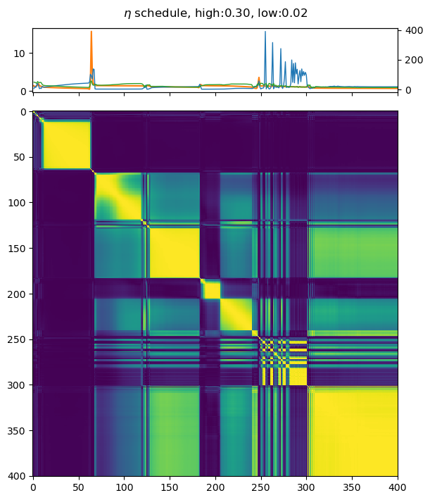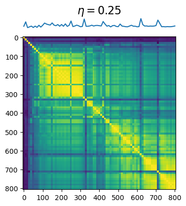We show in the Appendix that, in many cases, using $m=1$ , leads to poor similarities, which suggests that there exists $m\ll n$ where $|S(V^{*}_{t_{0}},V^{*}_{t})|<\epsilon$ for some $\epsilon$ .

We turn to the effect of $\eta$ on landscape shift. In Fig. 3, we plot the $S(V^{*}_{p},V^{*}_{q})$ where $p,q$ are taken from the entire trajectory. The initialisation is identical for each trajectory, and for this particular initialisation, the unstable regime of learning begins at $\eta=0.03$ . Using the smooth $\eta=0.01$ trajectory as a baseline, we see that the trajectory of low $\eta$ are largely similar as we enter the unstable regime. Eventually, the windows of similarity become more local when $\eta$ is large, showing that the "effective" parameters of the Hessians change across instabilities. Given the connection between "effective" parameters and solutions, this suggests that large learning rates encourage the exploration of new solutions.

Alternatively, we use $\eta=0.01$ as a baseline to compare trajectories across learning rates via gradient and Hessian similarities. These results are plotted in Fig. 4. We note the extraordinary similarity between $\eta=0.05$ and $\eta=0.01$ , where the Hessian rotation and gradient directions are largely similar, and $|g|$ is identical when it recovers from instabilities. As $\eta$ is increased, the trajectories become less similar to the baseline, until $\eta=0.20$ beyond which the trajectories become extremely dissimilar. The similarity of trajectories with $\eta$ to the smooth baseline supports the view that low learning rates tend to preserve existing solutions.

4 Discussion

In this work, we describe the phases of gradient descent instabilities. Our observations highlight landscape flattening and landscape shift across different learning rates. As we observe landscape flattening and landscape shift, the constancy of landscape orientation and validation loss provides further evidence for the connection between "effective" parameters and generalisation. Intuitively, we can view landscape shifts at low $\eta$ to be a re-ordering of "effective" parameters, which is ineffectual to model performance as $V^{*}$ is not shifted.

Our experiments build toward a body of studies characterising the behaviour of gradient descent at large learning rates as the relationship between large learning rates and generalisation attracts increasing attention. Following Cohen et al. (2022), our work further shows that there exist large $\eta$ s that do not cause divergence but may introduce significant changes to the orientation of the loss landscape where consistent a decrease in the training objective over long timescales may not be guaranteed. Progressive sharpening Cohen et al. (2022) offers an explanation for the heating phase, the mechanisms of the cooling phase are less well studied and our experiments add to the body of evidence for its understanding. Lewkowycz et al. (2020) shows that for low but unstable $\eta$ s, optimisers are "catapulted" around during training instabilities, which is supported by landscape flattening.

Our work presents an initial foray into the description of learning dynamics with large learning rates, but a complete understanding has some way to go. A better taxonomy and understanding of these regimes could speed up optimisation for practitioners using gradient methods for deep networks. We exploited the connection between Hessian eigen-directions to problem-specific degrees-of-freedom, so strengthening this connection would be beneficial toward generalisation. We see information compression and the variance of the bulk Hessian playing crucial, but under-explored, roles in this connection.

References

Bradbury et al. (2018) James Bradbury, Roy Frostig, Peter Hawkins, Matthew James Johnson, Chris Leary, Dougal Maclaurin, George Necula, Adam Paszke, Jake VanderPlas, Skye Wanderman-Milne, and Qiao Zhang. JAX: composable transformations of Python+NumPy programs, 2018. URL http://github.com/google/jax.
Brown et al. (2020) Tom B. Brown, Benjamin Mann, Nick Ryder, Melanie Subbiah, Jared Kaplan, Prafulla Dhariwal, Arvind Neelakantan, Pranav Shyam, Girish Sastry, Amanda Askell, Sandhini Agarwal, Ariel Herbert-Voss, Gretchen Krueger, Tom Henighan, Rewon Child, Aditya Ramesh, Daniel M. Ziegler, Jeffrey Wu, Clemens Winter, Christopher Hesse, Mark Chen, Eric Sigler, Mateusz Litwin, Scott Gray, Benjamin Chess, Jack Clark, Christopher Berner, Sam McCandlish, Alec Radford, Ilya Sutskever, and Dario Amodei. Language models are few-shot learners, 2020.
Cohen et al. (2022) Jeremy M. Cohen, Simran Kaur, Yuanzhi Li, J. Zico Kolter, and Ameet Talwalkar. Gradient descent on neural networks typically occurs at the edge of stability, 2022.
Foret et al. (2020) Pierre Foret, Ariel Kleiner Google Research, Hossein Mobahi Google Research, and Behnam Neyshabur Blueshift. Sharpness-aware minimization for efficiently improving generalization. 10 2020. 10.48550/arxiv.2010.01412. URL https://arxiv.org/abs/2010.01412v3.
Fukushima (1975) Kunihiko Fukushima. Cognitron: A self-organizing multilayered neural network. Biol. Cybern., 20(3–4):121–136, sep 1975. ISSN 0340-1200. 10.1007/BF00342633. URL https://doi.org/10.1007/BF00342633.
Ghorbani et al. (2019) Behrooz Ghorbani, Shankar Krishnan, and Ying Xiao. An investigation into neural net optimization via Hessian eigenvalue density. 36th International Conference on Machine Learning, ICML 2019, 2019-June:4039–4052, 1 2019. 10.48550/arxiv.1901.10159. URL https://arxiv.org/abs/1901.10159v1.
Granziol (2020) Diego Granziol. Flatness is a false friend, 2020.
Granziol et al. (2020) Diego Granziol, Stefan Zohren, Stephen Roberts, and Simon Lacoste-Julien. Learning rates as a function of batch size: A random matrix theory approach to neural network training. Journal of Machine Learning Research, 1:1–48, 2020.
Hochreiter and Schmidhuber (1997) Sepp Hochreiter and Jürgen Schmidhuber. Flat Minima. Neural Computation, 9(1):1–42, 01 1997. ISSN 0899-7667. 10.1162/neco.1997.9.1.1. URL https://doi.org/10.1162/neco.1997.9.1.1.
Hoffer et al. (2018) Elad Hoffer, Itay Hubara, and Daniel Soudry. Train longer, generalize better: closing the generalization gap in large batch training of neural networks, 2018.
Hunter (2007) J. D. Hunter. Matplotlib: A 2d graphics environment. Computing in Science & Engineering, 9(3):90–95, 2007. 10.1109/MCSE.2007.55.
Izmailov et al. (2019) Pavel Izmailov, Dmitrii Podoprikhin, Timur Garipov, Dmitry Vetrov, and Andrew Gordon Wilson. Averaging weights leads to wider optima and better generalization, 2019.
Kaur et al. (2022) Simran Kaur, Jeremy Cohen, and Zachary C Lipton. On the maximum Hessian eigenvalue and generalization. 2022.
Keskar et al. (2017) Nitish Shirish Keskar, Dheevatsa Mudigere, Jorge Nocedal, Mikhail Smelyanskiy, and Ping Tak Peter Tang. On large-batch training for deep learning: Generalization gap and sharp minima, 2017.
Kingma and Ba (2017) Diederik P. Kingma and Jimmy Ba. Adam: A method for stochastic optimization, 2017.
Krizhevsky and Hinton (2009) Alex Krizhevsky and Geoffrey Hinton. Learning multiple layers of features from tiny images. Technical Report 0, University of Toronto, Toronto, Ontario, 2009.
Krizhevsky et al. (2012) Alex Krizhevsky, Ilya Sutskever, and Geoffrey E. Hinton. Imagenet classification with deep convolutional neural networks. In Proceedings of the 25th International Conference on Neural Information Processing Systems - Volume 1, NIPS’12, page 1097–1105, Red Hook, NY, USA, 2012. Curran Associates Inc.
Lanczos (1950) Cornelius Lanczos. An iteration method for the solution of the eigenvalue problem of linear differential and integral operators. J. Res. Natl. Bur. Stand. B, 45:255–282, 1950. 10.6028/jres.045.026.
LeCun et al. (1992) Yann LeCun, Patrice Simard, and Barak Pearlmutter. Automatic learning rate maximization by on-line estimation of the Hessian's eigenvectors. In S. Hanson, J. Cowan, and C. Giles, editors, Advances in Neural Information Processing Systems, volume 5. Morgan-Kaufmann, 1992. URL https://proceedings.neurips.cc/paper_files/paper/1992/file/30bb3825e8f631cc6075c0f87bb4978c-Paper.pdf.
Lewkowycz et al. (2020) Aitor Lewkowycz, Yasaman Bahri, Ethan Dyer, Jascha Sohl-Dickstein, and Guy Gur-Ari. The large learning rate phase of deep learning: the catapult mechanism, 2020.
Li et al. (2018) Hao Li, Zheng Xu, Gavin Taylor, Christoph Studer, and Tom Goldstein. Visualizing the loss landscape of neural nets, 2018.
MacKay (1992) David J.C. MacKay. Bayesian methods for adaptive models, 1992.
Maddox et al. (2020) Wesley J. Maddox, Gregory Benton, and Andrew Gordon Wilson. Rethinking parameter counting in deep models: Effective dimensionality revisited, 2020.
Nesterov (2014) Yurii Nesterov. Introductory Lectures on Convex Optimization: A Basic Course. Springer Publishing Company, Incorporated, 1 edition, 2014. ISBN 1461346916.
Papyan (2019a) Vardan Papyan. Measurements of three-level hierarchical structure in the outliers in the spectrum of deepnet Hessians, 2019a.
Papyan (2019b) Vardan Papyan. The full spectrum of deepnet Hessians at scale: Dynamics with SGD training and sample size, 2019b.
Papyan (2020) Vardan Papyan. Traces of class/cross-class structure pervade deep learning spectra. Journal of Machine Learning Research, 21(252):1–64, 2020. URL http://jmlr.org/papers/v21/20-933.html.
Pearlmutter (1994) Barak A. Pearlmutter. Fast Exact Multiplication by the Hessian. Neural Computation, 6(1):147–160, 01 1994. ISSN 0899-7667. 10.1162/neco.1994.6.1.147. URL https://doi.org/10.1162/neco.1994.6.1.147.
Sagun et al. (2017) Levent Sagun, Leon Bottou, and Yann LeCun. Eigenvalues of the Hessian in deep learning: Singularity and beyond, 2017.
Vaswani et al. (2017) Ashish Vaswani, Noam Shazeer, Niki Parmar, Jakob Uszkoreit, Llion Jones, Aidan N. Gomez, Lukasz Kaiser, and Illia Polosukhin. Attention is all you need, 2017.
Wang and Roberts (2023) L. Wang and S.J. Roberts. SANE: the phases of gradient descent through sharpness aware number of effective pamareters. 2023.
Xiao et al. (2017) Han Xiao, Kashif Rasul, and Roland Vollgraf. Fashion-MNIST: a novel image dataset for benchmarking machine learning algorithms, 2017.
Ye and Lim (2016) Ke Ye and Lek-Heng Lim. Schubert varieties and distances between subspaces of different dimensions, 2016.

Appendix A Experimental details

In this section, we detail the technical details used in the experiments in the main sections.

Lanczos iteration. We can get the HVP using Pearlmutter (1994)’s trick, and we use the Lanczos (1950) algorithm for our Hessian $\mathcal{H}$ computations. Let the number of Lanczos iterations be $n_{\mathrm{L}}$ , the algorithm returns a tridiagonal matrix $T\in\mathcal{R}^{n_{\mathrm{L}}}\times\mathcal{R}^{n_{\mathrm{L}}}$ . We use $n_{\mathrm{L}}=100$ , and the eigenvalues of the smaller $100\times 100$ tridiagonal matrix can be readily computed using existing numerical libraries (e.g. numpy). The eigenvectors of $\mathcal{H}$ can be computed easily, $V=V_{T}^{T}V_{\mathrm{L}}$ , where $V_{T}$ are the eigenvectors of the tridiagonal matrix $T$ and $V_{L}$ the Lanczos vectors as secondary outputs from the algorithm. We perform re-orthogonalisation on the matrix of Lanczos vectors after every iteration. Our implementation of jax-powered Bradbury et al. (2018) Lanczos references a baseline implementation from https://github.com/google/spectral-density.

FMNIST. We train 5-layer MLPs with 32 hidden units in each layer for classification on the FMNIST dataset with cross-entropy loss. Our neural layers use ReLU activation, introduced by Fukushima (1975). As pointed out by Granziol et al. (2020), the batch size $b$ of data can influence the sharpness of the landscape up until a regime of large $b$ where the eigenvalue from $\mathcal{H}_{\mathrm{emp}}$ dominates the scaling term. Following these intuitions, we compute optimal batch-size $b$ for FMNIST, and found that beyond $b=1000$ , the Hessian at initialisation did not reduce significantly in sharpness. This implies that $\mathcal{H}_{\mathrm{batch}}$ is no longer dominated by the scaling term and so is a $\lambda_{i,b}\approx\lambda_{i,\mathrm{emp}}$ . As a result, $b=1000$ represents our full training dataset on FMNIST. To ensure classes are well-represented in the training dataset, we construct the dataset with the first $4$ classes of FMNIST, so that each class will be represented by $\sim 250$ instances in the training dataset. The evaluation set is the same size, $b_{\mathrm{eval}}=1000$ . For $\hat{d_{m}}$ , we use $m=4$ equal to the number of classes in the classification problem.

CIFAR-10. We train modified versions of AlexNet, introduced by Krizhevsky et al. (2012), on CIFAR-10 with cross-entropy loss. The network architecture uses $2$ sets of convolution & max-pool blocks. Convolution layers are structured as ( $64$ features, $(5,5)$ kernel, $(2,2)$ strides) and max-pool as ( $(3,3)$ kernel). This structure is followed by $2$ dense (fully-connected) layers with $382$ and $196$ hidden units respectively, and finally an output layer, following the modifications of Keskar et al. (2017). Our model uses ReLU activation Fukushima (1975). Similar to FMNIST, we computed an optimal reduced batch size from the full training set, in this case, $b=5000$ . All $10$ classes are used in this task, so each class is represented by $\sim 500$ instances in the training dataset. The evaluation set is smaller, $b_{\mathrm{eval}}=1000$ . All models were trained to $1000$ epochs.

Appendix B Phases of learning on FMNIST, higher $\eta$

Section 3 presented our claims with detailed computations on FMNIST. In this section, we show the phases of learning at higher learning rates in Fig. LABEL:fig:fmnist-more, and we look at different choices of $m$ to compute $S(V^{*}_{p},V^{*}_{q})$ in Fig 6. The reordering effect is clearer for higher $\eta$ , where high misalignments are observed for lower $m$ .

Appendix C Phases of learning on CIFAR-10

Section 3 presented our claims with detailed computations on FMNIST. In this section, we show the phases of learning on CIFAR-10 Krizhevsky and Hinton (2009), a more challenging dataset for image classification. To scale our computation to deep neural nets, we present an approximation to the full Hessian that exploits the natural ordering of neural weights. We justify this approximation in detail in Appendix section D

Approximation to the full Hessian. We parameterise a prediction function $\hat{y_{i}}=f_{\theta}(x_{i})$ with a deep neural net with weights $\theta$ . Let the network have layers and outputs ( $\phi_{k}$ , $T_{k}$ ), $k=1,2,...n_{\phi}$ , ordered from the output layer such that $\phi_{k+1}(T_{k+1},\theta_{k+1})=T_{k}$ and $T_{n_{\phi}}=\textbf{x},T_{0}=f_{\theta}(\textbf{x})$ , then $f_{\theta}(x_{i})=\phi_{1}(\phi_{2}(...(\phi_{n_{\phi}}(x_{i}))))$ . We consider the reduced objective $\mathcal{L}^{\mathrm{r}}_{\theta(k)}=\mathbb{E}_{\bm{T}_{k}}L_{\theta(k)}(\bm{T}_{k})$ , where $\theta(k)=[\theta_{1},\theta_{2},...,\theta_{k}]$ to compute the reduced Hessian $\mathcal{H}^{\mathrm{r}}_{k}=\gradient^{2}_{\theta(k)}\mathcal{L^{\mathrm{r}}}_{\theta(k)}$ . In other words, we approximate the Hessian of the full deep neural network with a Hessian computed on the first $k$ layers closest to the output layer. Empirically, this approximation changes the absolute scale of the resulting eigen-spectrum, but the relative scales of measures along the training trajectory are accurate.

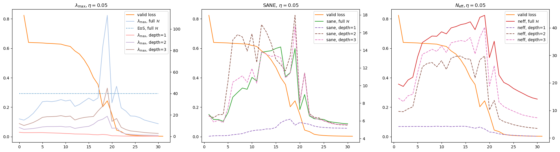
Experiments on CIFAR-10. Fig. 7 shows a specific training trajectory, where we initially observe a large amount of noise. After epoch 700, the trajectory displays the structure of phase transitions, and we visualise the details in Fig. 7(b) across depths $k=1,2,3$ , where $k=1$ is the output layer only. For each depth, the percentage of model parameters included in the computation was $0.2\%,9.7\%,86.5\%$ , showing that a more accurate approximation of the full Hessian as $k$ is increased. We note the significant difference in $k=1$ computations vs $k=2,3$ , and we note that the output layer is unique in its lack of an activation function. Sadly, we were not able to compute $\overline{S(v)}$ given the limit of GPU memory. We note the clear phases as shown by loss and the measures SANE $N_{\mathrm{eff}}$ and $\lambda_{\mathrm{max}}$ with the corresponding peaks and troughs as described in Section 3. However, the insight of Hessian rotations through $\overline{S(v)}$ and $|g(\theta_{k})|$ is not clear, though we note the remarkable similarity of $|g(\theta_{k})|$ and $\overline{S(g)}$ across depths.

Appendix D Additional synthetic experiments

In this section, we establish the connection of eigenvectors to specific degrees-of-freedom that control performance and generalisation, and we visualise the behaviour of the $k$ -layer approximation to the full Hessian introduced in Section C. Owing to the excessive amounts of compute required for larger datasets and models, we validate these observations on two small synthetic datasets - one for regression and one for classification. Synthetic datasets have the added benefit of allowing a lower dimensional input space to enable more intuitive visualisations of regression predictions and classification boundaries. The regression task fits the function $f(x)=4x\sin(8x)$ , which makes a W-shape in the domain $[-1,1]$ , we call this dataset W-reg. For classification, we use a Swiss-Roll (SRC) dataset which represents a complex transformation from the two-dimensional input space to the feature space. These synthetic datasets are plotted in Fig. 8.

D.1 "Effective" parameters control important degrees-of-freedom

Perturbations. We train MLPs for both W-reg and SRC using MSE and cross-entropy loss at large $\eta$ s. Taking models at the final epoch, we visualise the specific degrees-of-freedom (d.o.f.s) corresponding to the top $n=6$ eigenvectors of the Hessian. These d.o.f.s are evaluated through perturbation theory, allowing us to perturb the model weights along the eigen-directions and measure the effect on output space. The weights are perturbed as $\theta_{p,i}=\theta\pm p_{i}v_{i}$ , where $p$ is a scaling factor. Perturbations on eigen-directions of the full-model Hessian, as well as with $k$ -layer approximations of varying depths, are shown in Fig. 9. In a full-batch and large $\eta$ regime, we expect the sharpness of final models to be determined by the unstable dynamics of gradient descent and by the Edge of Stability. As $\lambda$ s get increasingly sharp, the landscape in the two-dimensional plane defined by $[v,\mathcal{L}]$ gets increasingly sharp, and so we use a square-root scaling factor (based on the quadratic assumption) $p_{i}=|\lambda_{i}|^{\frac{1}{2}}c_{p}$ . The positive and negative perturbations form the boundaries of the error bars of the visualisations.

W regression. Focusing on the top subplot of the top plot of Fig. 9, we can qualitatively attribute the components of the regression solution to the specific eigenvectors. From the edges, $v_{1}$ controls the local d.o.f. of the left edge of the desired output, and $v3$ is the right. Moving inwards, the second bend from both the left and right are controlled by $v_{2}$ and $v_{4}$ respectively. $v_{2}$ also controls the middle plateau, and $v_{5}$ , $v_{6}$ offer more precise tuning for the sharp turns at the bottom of the W shape. We find it surprising that the sharpest eigen-directions appear to control salient d.o.f.sthat correspond to performance in the local region, and that these sharpest eigenvectors form a ’sum of local parts’ to generate the whole solution. We note that the ordering of $v_{1}$ , $v_{2}$ , and $v_{3}$ is coincidentally similar to the frequency of datapoints in the training set within the respective regions of the input domain. Since the empirical Hessian is driven by the loss from training samples, it is possible that the relative sharpness of $v$ s are determined by the frequency of the corresponding feature in the training set.

Swiss-Roll classification. The perturbations plots for SRC are shown in the top subplot of the bottom plot of Fig. 9. The red and green show the ’unperturbed’ decision boundaries, while the error bars on the classification boundary due to perturbation have a blue fill. Given the more landscape compared to W-reg, we note that the sharpest eigen-directions of the Hessian correspond to features that are local ( $v_{1}$ , $v_{2}$ , $v_{6}$ , and arguably $v_{3}$ ). $v_{4}$ and $v_{5}$ focus on the boundaries between the swirls - while they look similar in shape, the regions of uncertainty for each feature differ and are complementary.

D.2 The $k$ -layer approximation of the Hessian maintains relative scaling

In section C, we introduced the $k$ -layer approximation to the Hessian $\mathcal{H}^{\mathrm{r}}_{k}$ that exploits the natural ordering of weights. In Fig. 10 we compare metrics (SANE, $N_{\mathrm{eff}}$ , $\lambda_{\mathrm{max}}$ ) computed from $\mathcal{H}^{\mathrm{r}}_{k}$ to those from $\mathcal{H}$ , the full Hessian, on synthetic datasets. In Fig. 9, we perturb the eigenvectors computed from $\mathcal{H}^{\mathrm{r}}_{k}$ at different depths. From the empirical evidence, we observe that the relative scales of the metrics computed from $\mathcal{H}^{\mathrm{r}}_{k}$ follow metrics from the full Hessian. This observation was utilised in Section C to provide a connection between metrics from $\mathcal{H}^{\mathrm{r}}_{k}$ to model performance since only the relative scales along the trajectory are critical. Secondly, we note that the absolute scale of metrics computed from $\mathcal{H}^{\mathrm{r}}_{k}$ approaches those from $\mathcal{H}$ as $k$ is increased, which agrees with intuitions. As with Section 3, more work is required for an interpretation of the absolute values of SANE $N_{\mathrm{eff}}$ , and $\lambda_{\mathrm{max}}$ . Thirdly, we note that $\mathcal{H}^{\mathrm{r}}_{k}$ using only the output layer, i.e. $k=1$ , computes metrics that are highly uninformative. The low $\lambda_{\mathrm{max}}$ indicates a flat landscape. Despite this, the eigenvectors from $\mathcal{H}^{\mathrm{r}}_{k}$ $k=1$ correspond to local d.o.f.sthat are very similar to that of the full model, and we conjecture that the eigenvectors of the output layer exert significant control on the specific d.o.f.sfor eigenvectors approximated with more layers or from the full model.

Appendix E Additional studies

E.1 Hessian shifts with cyclic learning rates

We study the exploration of loss landscapes under six cyclic $\eta$ schedules through the similarity of $v_{\mathrm{max}}$ . We take $\eta_{+}\in(0.10,0.20,0.30)$ , situated well within the unstable regime, as the upper limits of our schedule; $\eta_{-}\in(0.02,0.05)$ are used as the lower limits. $\eta=0.02$ is in the smooth earning regime while $\eta=0.05$ is unstable. These cyclic $\eta$ schemes use $\eta_{+}$ for $10$ epochs, before switching to $\eta_{-}$ for $50$ epochs and repeating. The final $40$ epochs use $\eta_{-}$ . The results are visualised in Fig. 11, and we see difference choices of $\eta_{+}$ and $\eta_{-}$ can lead to different movements of the Hessian. We observe that large $\eta_{+}$ s encourage Hessian shifts. Surprisingly, it is not the case that using low $\eta_{+}$ and $\eta_{-}$ will lead to stagnation in similar loss landscapes. The ratio $\frac{\eta_{+}}{\eta_{-}}$ appears to play an important role.