The inhomogeneous multispecies PushTASEP: Dynamics and symmetry
Abstract.
We introduce and study a natural multispecies variant of the inhomogeneous PushTASEP with site-dependent rates on the finite ring. We show that the stationary distribution of this process is proportional to the ASEP polynomials at and . This is done by constructing a multiline process which projects to the multispecies PushTASEP, and identifying its stationary distribution using time-reversal arguments. We also study symmetry properties of the process under interchange of the rates associated to the sites. These results hold not just for events depending on the configuration at a single time in stationarity, but also for systems out of equilibrium and for events depending on the path of the process over time. Lastly, we give explicit formulas for nearest-neighbour two-point correlations in terms of Schur functions.
Key words and phrases:
PushTASEP, multispecies, inhomogeneous, multiline, TASEP, interchangeability2010 Mathematics Subject Classification:
60J10, 82B20, 82B23, 82B44, 33D52, 05A101. Introduction
The multispecies asymmetric simple exclusion process (ASEP) is an interacting particle system originating in statistical mechanics and probability, with significant connections to different areas of mathematics such as combinatorics and representation theory. It has been the focus of considerable study in the last few decades. The stationary distribution of the multispecies TASEP (i.e. ASEP with asymmetry parameter ) on a ring of size was described by Ferrari and Martin [ferrari-martin-2007] in terms of multiline diagrams. The connection between the multispecies ASEP with content and the Macdonald polynomial was realised by Cantini–de Gier–Wheeler [cantini-degier-wheeler-2015] and by Chen–de Gier–Wheeler [chen-degier-wheeler-2020]. In these works, they define ASEP polynomials (which are called relative Macdonald polynomials in [guo-ram-2021], and which are special cases of the permuted basement Macdonald polynomials studied in [ferreira-2011, alexandersson-2019]). These are polynomials in variables whose coefficients are rational functions in , which, for and all equal, are proportional to the stationary distribution of the multispecies ASEP. Later on, Corteel–Mandelshtam–Williams [corteel-mandelshtam-williams-2022] showed that the ASEP polynomials can be computed using the multiline diagrams stated above by assigning a weight depending on and the variables .
The ASEP itself is not thought to have nice algebraic properties when the jump rates are allowed to differ between sites – but it is natural to ask if there is some multispecies particle system with site-wise inhomogeneity whose stationary distribution is proportional to the ASEP polynomial at for general values of the parameters .
In this and a companion paper [ayyer-martin-williams-2024], we show that this is indeed the case, for a multispecies inhomogeneous version of the PushTASEP, with deformation parameter . The case of general is covered in [ayyer-martin-williams-2024]. In this work, we focus on various interesting aspects of the particular case .
The arguments in [ayyer-martin-williams-2024] involve developing relationships between the ASEP polynomials and the non-symmetric Macdonald polynomials. Here for the case , we explain an alternative proof of a different nature, constructing a Markov chain on multiline diagrams whose bottom row projects to the PushTASEP process, and whose stationary distribution is proportional to the weight defined in [corteel-mandelshtam-williams-2022]. This extends the approach of [ferrari-martin-2006] to the inhomogeneous setting.
A particular focus is on symmetry properties under interchange of the rates between different sites. We show that probabilities of events depending on a given interval of sites remain unchanged when the rates at other sites are permuted. Such results are proved for the general case in [ayyer-martin-williams-2024], for events depending on the configuration at a single time in the stationary distribution. In the special case we can prove significantly stronger properties, applying to systems out of equilibrium, and to events which depend not just on a single time but on the path of an evolving process. These results are obtained by using coupling methods to prove interchangeability results for PushTASEP stations analogous to those previously proved for exponential queueing servers [Weber1979, TsoucasWalrand1987, MartinPrabhakar2010].
Finally we study various observables for the system in stationary, such as the density of particles of a given species at a given site, and the current between sites for particles of a given species. We give explicit formulas for nearest-neighbour two-point correlations in terms of Schur functions.
The PushTASEP, although somewhat less widely known than its cousin the TASEP, has nonetheless been widely studied in recent years. Spitzer [spitzer-1970] introduced it as an example of a long-range exclusion process, but more recently the name PushTASEP has become established. It has often been studied on the infinite lattice – see for example [petrov-2020] for extensive references – but there have been a few studies on finite graphs as well [ayyer_schilling_steinberg_thiery.sandpile.2013, ayyer-2016]. The multispecies case was already considered in [ferrari-martin-2006], under the guise of the discrete-space Hammersley–Aldous–Diaconis process, to which it is equivalent by particle-hole duality. A related multispecies process in discrete time (dubbed the “frog model”) was recently used by Bukh–Cox [bukh-cox-2022] to study problems involving the longest common subsequence between a periodic word and a word with i.i.d. uniform entries. For an inhomogeneous version on the line, limit shape and fluctuation results are obtained by Petrov [petrov-2020]. The multispecies inhomogeneous model with was studied on an open interval by Borodin and Wheeler [borodin-wheeler-2022, Section 12.5].
As this project was being completed, related work by Aggarwal, Nicoletti and Petrov appeared [aggarwal-nicoletti-petrov-2023], which studies an inhomogeneous PushTASEP on the ring (in fact, a more general model in which the sites can have capacities greater than ). They obtain a description of the stationary distribution of such systems in terms of “queue vertex models” on the cylinder – these objects are closely related to multiline diagrams (and to matrix product formulae). Their methods are very different to ours, making extensive use of the Yang-Baxter equation.
1.1. Main results
We now describe the model we study, an inhomogeneous PushTASEP on a ring of size , with species of particle (called ).
We start with the single species case, i.e. . Each site contains either a single particle of type , or a vacancy. The number of particles will be conserved by the dynamics – write for the number of particles, and for the number of vacancies. Then a configuration is a tuple of length containing s and s, where if the configuration has a particle at .
We have positive real parameters , which we think of as attached to the sites . The system is a Markov chain whose rates can be described as follows. At each site , a bell rings at rate . When this bell rings, if is vacant, nothing changes. If is occupied by a particle, that particle moves to the first vacant site clockwise from , leaving a vacancy at itself.
Now we move to the general case of species. We denote if the configuration has a particle of type at site , where , and if site is vacant. The number of particles of each type will be conserved by the dynamics: write for the number of particles of species for – now the number of vacancies is .
Equivalently we can describe the particle content as a partition (i.e. a weakly decreasing tuple of non-negative integers) of length , given by
It will also be convenient to write in frequency notation as . Unless otherwise stated, we will fix throughout some partition giving the content of the system, with species of particles and length .
A configuration is then a permutation of , and may be thought of as a composition (i.e. a tuple of non-negative integers). We write for the set of all configurations, which is the state-space of the Markov chain. For example,
The dynamics of the multispecies chain are as follows; the idea is that higher-numbered species are “stronger” than lower-numbered species, and can displace them. As above, a bell rings at each site at rate . When such a bell rings, if , i.e. the site is vacant, nothing changes. Otherwise, suppose contains a particle of species . Then this particle moves to the first location clockwise from with . If this site was previously vacant (i.e. ), the jump is complete; otherwise the particle of type itself moves clockwise until it finds a site with . This game of ‘musical chairs’ continues, with stronger particles displacing weaker ones in turn, until a vacancy is found. All the particles involved move instantaneously to their chosen positions, leaving a vacancy at site .
An important observation is that the multispecies dynamics with species of particle can be seen as a coupling (the so-called “basic coupling”) of single-type PushTASEP processes. These can be obtained by regarding all species of type or higher as “particles” and all species of type or lower as “vacancies”, for any . See 7 at the end of Section 2 for more details.
To illustrate the dynamics, consider the configuration on sites with species. Then for example
| (1.1) |
If a bell rings either at site or at site rings, nothing changes.
The transition graph of the multispecies PushTASEP on is given in Figure 1.
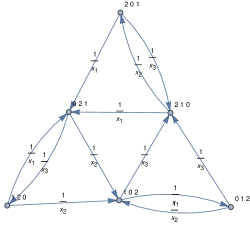
Note that when a bell rings at a given site in a given configuration, the transition it triggers is deterministic. (This will no longer be true in the case .)
We start with an explicit formula for the stationary distribution. To state it, we first recall that the elementary symmetric polynomial for is given by
| (1.2) |
For a partition , we define . We also need the notion of the ASEP polynomials, first defined in Cantini–de Gier–Wheeler [cantini-degier-wheeler-2015] and later named as such by Chen–de Gier–Wheeler [chen-degier-wheeler-2020], denoted . These are important nonsymmetric polynomials related to the well-known symmetric Macdonald polynomials . The ASEP polynomials, indexed by compositions , are polynomials in the variables , whose coefficients are rational functions in . We express the stationary distribution for a system with content using the family of ASEP polynomials where is a permutation of .
Theorem 1.
Let be a partition, and set for . The stationary distribution of the multispecies PushTASEP with content is given by
for , where is the ASEP polynomial and
is the partition function.
We discuss the ASEP polynomials further in Section 4, although we don’t give a full definition. For a definition in full generality, see for example [chen-degier-wheeler-2020, corteel-mandelshtam-williams-2022, ayyer-martin-williams-2024] for various approaches. If the reader prefers, 1 can instead be understood without any reference to ASEP polynomials, as a statement that the stationary probabilities are proportional to sums of weights of multiline diagrams, as defined in Section 4. See LABEL:thm:stat_prob_sum for a precise statement of the result in this form.
Note that in the homogenous case , the stationary distribution of the system is the same as for the multispecies TASEP, (as was already observed, more specifically for the system on the whole line, in [ferrari-martin-2006]).
LABEL:thm:stat_dist_multiline is a special case of the result proved in the more general case of the -PushTASEP for in [ayyer-martin-williams-2024], via relationships between ASEP polynomials and non-symmetric Macdonald polynomials; however the more probabilistic approach explained here via the multiline process and time-reversal also seems interesting in its own right.
Our second main result is about the invariance of the process under permutations of the parameters .
Theorem 2.
Consider the multispecies PushTASEP on the ring with content , started either in the stationary distribution, or in any starting configuration with in which .
The distribution of the path of the process observed on sites is invariant under permutations of the parameters .
An analogous property was recently proved for the multispecies TAZRP [ayyer-mandelshtam-martin-2022] using results about interchangeability of exponential-server queues in series. To prove 2, we need to develop similar interchangeability results in a new context where the exponential-server queues are replaced by PushTASEP stations.
A related symmetry property for events depending just on the configuration at a single time in stationarity is obtained in the general case in [ayyer-martin-williams-2024]. However the result of 2 is much stronger, both since it applies to systems out of stationarity, and since it applies to events which depend on the path of the process evolving over time. The question of whether this stronger symmetry property can also be extended to seems very interesting.
Finally, we look at various important observables for the PushTASEP stationary distribution. We will give formulas for the density and current of particles in LABEL:sec:obs, which can be derived from the corresponding results for a single species system. Unlike in the homogeneous case, even the density of a given species at a given site is not obvious. A more intricate result is a formula for the nearest-neighbour two-point correlation, which is our third main result. This generalizes results of Ayyer–Linusson for the multispecies TASEP [ayyer-linusson-2016] and Amir–Angel–Valko for the TASEP speed process [amir-angel-valko-2011].
For the purposes of this discussion, we will restrict ourselves to with species of particles (but all other cases can be derived from this case by projection).
To state the result, we recall that the Schur polynomial are an important family of symmetric polynomials playing a significant role in representation theory and algebraic geometry [stanley-ec2]. The Schur polynomial can be defined as a ratio of determinants,
| (1.3) |
which is symmetric in . For , define the polynomials
and
where if is negative.
Let denote the occupation variable for the particle of species at site , i.e., (resp. ) when the th site is occupied (resp. not occupied) by a particle of species (where “particle of species ” means a vacancy).
Theorem 3.
Let . Then the joint probability of seeing the particle of species at site and that of species at site is given by
The proof of 3 involves projecting from the multispecies system to a suitable -species system, for which the probabilities of relevant events can be analysed using -line diagrams.
Note that in all cases the two-point correlation function obtained in 3 is symmetric in , as must be the case in the light of 2. It is interesting to observe the appearance of the Schur polynomials in these expressions. In the homogeneous case, under suitable rescaling in the limit , one obtains interesting asymptotics for the joint distribution of the species observed at the two sites as shown in [amir-angel-valko-2011]; setting , one obtains a limit with constant density in the region , a singular term involving non-vanishing probability on the boundary , and repulsion from the boundary in the region . It would be interesting to explore asymptotics in regimes involving inhomogeneous parameters .
Note that the result of [ayyer-linusson-2016] has recently been extended in a different direction by Pahuja [pahuja-2023], who obtains nearest-neighbour two-point correlations for the multispecies ASEP (i.e. in our notation the case with all equal), based on the multiline diagram construction for the ASEP in [martin-2020].
The plan of the rest of the paper is as follows. Throughout, we consider the case of a multispecies PushTASEP whose contents are fixed and given by some partition . In Section 2, we will derive the stationary distribution for the single species inhomogeneous PushTASEP as well as formulas for the density and current; we also explain the interpretation of the multispecies system as a basic coupling of single species systems. In Section 3, we give a proof of the interchangeability of rates for the single species PushTASEP and use that to prove 2. In Section 4, we define multiline diagrams and construct a multiline process which will lump to the multispecies PushTASEP, in order to obtain the stationary distribution in 1. Finally, in LABEL:sec:obs, we will prove formulas for the current and the density as well as the formula for the two-point correlations in 3.
2. Single species PushTASEP
In this section, we focus on the PushTASEP with a single species of particle, i.e. . As before, we take sites. Therefore, with particles (and so vacancies) and periodic boundary conditions.
Recall that is the configuration space. For example, consider the case . With the lexicographic ordering of the configurations, i.e.,
the transition graph of the chain is given in Figure 2.
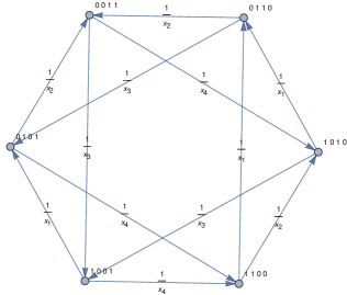
We are interested in the stationary distribution of this process. It is easy to see that the single species PushTASEP is irreducible. Therefore, the stationary distribution is unique. The the following proposition is straightforward to prove using the master equation.
Proposition 4.
The stationary probability of for the PushTASEP is
Recall that the density at site is the probability of finding a particle at site in the stationary distribution. We will use angular brackets to denote expectations in the stationary distribution. As is usual, we let be the indicator variable for a particle at site , so that is the density at site . Because of the factorized nature of the stationary distribution in 4, we immediately obtain the following.
Corollary 5.
The density at site in the stationary distribution is given by
where the hat on an argument denotes its absence.
The current of a particle across a given edge (say ) is the number of particles per unit time that cross that edge in stationarity. Because of particle conservation, the current is the same for all edges. We will denote the current by . In terms of the stationary distribution for the PushTASEP, this is given by
| (2.1) |
Proposition 6.
The current in the stationary distribution is given by
Proof.
Using arguments similar to the proof of 5, it is easy to see that
Plugging this into (2.1), we obtain, after setting ,
| (2.2) |
We now note an elementary recursive formula for the elementary symmetric function in (1.2). First, split this into terms according to whether appears or not to obtain
Now, successively apply this recurrence to each variable starting from and progressing up to , to get
One can check that the right hand side of this equation, after appropriate change of variables can be applied to (2.2). This gives the desired result. ∎
We have the following projection property for our multispecies dynamics. If we view all particles of species as “particles”, and all particles of lower species as vacancies, then we obtain a single species process with particles and vacancies.
Considering such projects for all , we can see the multispecies process as a coupling of single species processes. This is the basic coupling [liggett-1985, Chapter VIII, Section 2] (under which the bells ring at the same sites at the same types in all the coupled single species systems).
More generally, we can project from a “finer” multispecies system to another “coarser” one, allowing the merging of two or more adjacent classes into one:
Proposition 7.
Let be any function with which is weakly order-preserving (i.e. for all , ). Then the multispecies PushTASEP with particle content . lumps to the multispecies PushTASEP with particle content given by , where is the partition .
Proof.
This is an elementary consequence of the dynamics. We “recolour” the particles of the system, giving any particle previously of species the new label . It is an easy case-analysis to check that for any transition (caused by a bell at some site ), the result is independent of whether the recolouring is performed before or after the transition. For example, consider the system with content and the second transition in (1.1). Applying the map given by , , , we recolour to the system with content ,and the transition becomes in either case. ∎
To map to a single species system as described just above, we would apply the map with for , and for .
3. Interchangeability of rates
Weber [Weber1979] proved an interchangeability result for exponential queueing servers in tandem. Consider two independent queueing servers (i.e. servers who offer service at the times of a Poisson process) in tandem, with service rates and . The first queue has some arrival process , with an arbitrary distribution (for example, it could be deterministic), which is independent of the service processes. By “tandem” we mean that a customer leaving the first queue immediately joins the second queue; the departure process from the first server is the arrival process of the second.
Then Weber’s result is that the law of the departure process from the system (i.e. of the departure process from the second queue) is the same if the rates and are interchanged.
Various different proofs of this result were subsequently given; a significant one from our point of view was a coupling proof by Tsoucas and Walrand [TsoucasWalrand1987]. They constructed a coupling of two pairs of independent Poisson processes, with rates and with rates , such that for any arrival process , the output of the system with arrival process and service processes is the same as that of the system with arrival process and serice processes .
This stronger result, holding simultaneously for all arrival processes, makes it possible to extend to a multispecies framework (since, along the lines we have already seen above, a multispecies configuration can be seen as a coupling of several single species configurations). See for example [MartinPrabhakar2010] for extensive discussion and applications.
In this section we develop similar ideas in a new context, to obtain interchangeability of rates of PushTASEP stations. We will ultimately be able to apply them to get the result of 2.
We consider the PushTASEP on the ring for this work, but the result below applies equally to any one-dimensional lattice (such as a closed or open interval or all of ). Each site has an associated parameter . Bells ring independently as Poisson processes at each site, with rate at site . Recall that when a bell rings at site in the single species PushTASEP:
-
•
if is empty, nothing happens.
-
•
if is occupied, then:
-
–
becomes empty;
-
–
the first empty site to the right of becomes occupied;
which we call a transfer of a particle from to .
-
–
For each lattice bond , we have a “flux process” across the bond; a point process which records the times when there is a transfer of a particle from or a site to its left to or a site to its right.
Fix a site . Consider the system started from, say, time . If we know the flux process for the bond on the left of , the initial occupancy of the site , and the Poisson process of bells at site , then we can obtain the flux process for the bond on the right of .
Iterating, this now works for any finite interval , where . Given the flux process at the left end of the interval, the initial configuration inside the interval, and the bell processes inside the interval, one can obtain the flux process at the right end. For the moment we only need the case .
We write to denote a Poisson process with rate . This is our interchangeability result.
Theorem 8.
Consider two neighbouring sites , with parameters . Regard the output flux process on the time-interval as a function of:
-
•
the input flux process on ;
-
•
the Poisson processes and of bells at sites and respectively;
-
•
the time- occupancies of sites and , denoted by .
Then there exists a coupling of
| and | ||||
with the property that for every locally finite , and for every ,
with probability .
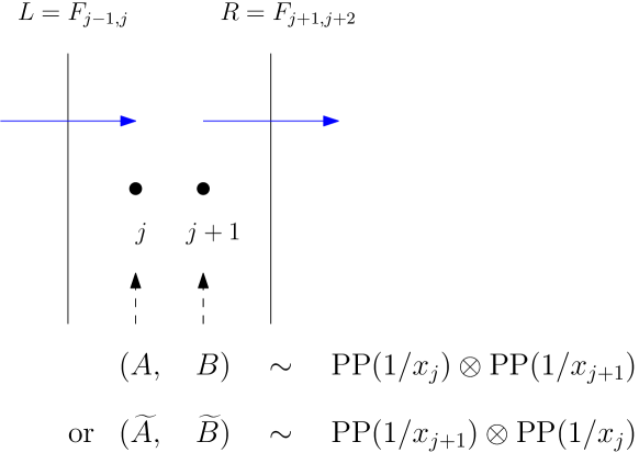
See Figure 3 for an illustration. This theorem says that the bell rates and at the neighbouring sites and are interchangeable.
Before we begin the proof, we describe the coupling. First, we will use and in the rest of this section to keep the notation simple. Recall that a basic fact about Poisson process is the thinning theorem [durrett-2016], which in our context reads as follows. We can describe via a single Poisson process of rate which is the superposition of and , with a mark or attached to each point, according to whether it comes from the process or respectively. Given the points of , the marks are i.i.d. and each is with probability and with probability . If we index the points of with in increasing order, say with point the last to occur before time and point the first to occur after time , then we can identify the sequence of marks with an element .
Under our coupling, the superposition will be the same as ; we will just change (some of) the marks. Consider occurrences of the motif , that is, look for such that , . The set of such has a distribution which is invariant under interchanging and . This is because if , then is equal to if for some , and otherwise is equal to . This means there exists a coupling of and with the required distributions such that:
-
•
the superpositions and are the same;
-
•
the occurrences of the motif are the same in both processes.
These are the only properties we will need, but we can make the coupling explicit as follows. The motifs are separated by words of the form , consisting of some number (maybe ) of ’s followed by some number (maybe ) of ’s. Conditional on the length of the string, the probability that it consists of ’s followed by ’s (where , with ) is proportional to
| (3.1) |
An explicit way to realise the coupling is to obtain the process from as follows. Leave the motifs unchanged. As for the separating them, replace it instead by . This is illustrated in Figure 4. Because of (3.1), this has the effect of interchanging the probability of and as desired.
Remark 9.
Equivalently, rather than using this deterministic scheme, one could just resample each of the strings independently according to the new desired measure. One can also think about all of this in terms of run lengths of consecutive ’s and ’s (which are independent, geometric () for the ’s and geometric() for the ’s).

Proof of 8.
We will consider two systems – call them and . In each one we have two sites and . We have the same input flux process . We have bell processes at and respectively given by and in system , and and in system . The claim is that the output flux processes are exactly the same (not just the same in distribution) in both systems.
The initial configuration is the same in both systems, with being one of , , or . See 10 after this proof for discussion of why cannot be . Since the flux into on the left is the same in the two systems, and they start with the same number of particles, in order to conclude that the flux out of on the right is the same in the two systems it will be enough to observe that the number of particles in these two sites remains the same across both systems for all times.
We work by induction to determine whether there could be a first moment when the number of particles in and do not agree. Let us first check whether an extra particle could be added in one system and not in the other. This could happen only when a point of occurs. But a point of always adds a particle unless the system is occupied in both and . So if a point of adds a particle in one system but not the other, it can only be because the numbers already didn’t agree.
Hence it would have to be that one system loses a particle, while the other does not. This would have to happen due to a bell ringing at either or . Recall that such bells happen simultaneously in and , though not necessarily in the same place (that is, the superpositions and are the same). First suppose both systems were previously full. Then any such bell loses a particle from both systems. So, the only way for the numbers to become unbalanced would be for both systems to contain one particle, and then for one of them (but not the other) to become empty. We will now show that both systems necessarily become empty at the same time.
This boils down to a case analysis. First, take the case where at time these two sites are full (i.e. ), or in the state . In this case, for the system to be empty at a given time, it is necessary and sufficient that since the last point of (or since time if there has been no point of ), there has been a bell at followed by a bell at . That is, we need to have observed the motif in the marks of the Poisson process. But our coupling ensures that this motif occurs at identical times in the systems and . The case where the system starts empty (i.e. ) is similar. In this case, if there has been no point of , then the system remains empty. If there has been a point of , then as above, for the system to be empty we need to have seen the motif since the last such point.
Hence the number of particles in the two systems and must remain the same at all times. It follows that the output flux processes and are the same, as desired. ∎
Remark 10.
The proof above fails, as it must, if instead we start from the configuration . Then if we observe a bell at in one system, but at in the other, then the former may have a point of the output flux process, while the latter does not.
Remark 11.
In the setting above we can also take the “input process” to be defined on all times in , and similarly obtain an output process for all times in . (This works straightforwardly since there are arbitrarily early times when we know the occupancy state of ; whenever the bell at rings, it becomes empty.) Then we may regard a single PushTASEP site as an operator which maps distributions of input processes to distributions of output processes. Recalling Burke’s theorem for exponential-server queues, we can ask whether all the ergodic fixed points of this map to be Poisson processes.
The fact that our coupling of and works simultaneously over all input processes means that we can pass from a single species result to a multispecies result.
Proof of 2.
First consider a single species PushTASEP on a ring of sites, with particles for some .
Imagine two versions and with the same initial configuration of this system, with the rates and at sites and swapped between the two. We may couple and using identical bell processes between the two systems everywhere except and , and using the coupling provided by 8 for the bell processes at sites and .
Suppose we start the two systems in the same configuration at time , with the configuration at sites being one of , or . Imagining the two systems evolving one bell at a time, we can see there is never a first moment when the flux processes and are different between the two systems. One minor subtlety can arise on the ring if there are particles. A bell at site can “cause” a push which propagates almost all the way around the ring, to create a point in the flux process . For this to happen, both systems must be in state on the sites , and both must experience a bell at . Afterwards they are both in state on those two sites, and the coupling between the two systems proceeds without problem.
Now we proceed to the multispecies PushTASEP on the ring of size . We view the multispecies PushTASEP as a coupling of several single species PushTASEPs. We take some initial condition on the multispecies system in which the particle at site is at least as strong as the particle at site . This means that in all the single species projections, the configuration at is in . Again we consider a coupling between two systems with rates or at and respectively, with all the other rates remaining the same. As before we use the coupling of the bell processes at sites and given by 8, and at all other sites, we keep the bell processes identical between the two systems. Since all the single species projections look the same between the two systems outside , the same is true of the multispecies system which is the coupling of those single species systems.
Now as in the statement of 2, we may fix any , and consider an initial condition in which . From the argument above, we may exchange the parameters of any two neighbouring sites in while preserving the distribution of the process as observed on sites . But then we can perform a sequence of such nearest-neighbour transpositions to realise any desired permutation of the parameters . So indeed the distribution is symmetric under permutation of these parameters, as desired.
Finally we wish to show the same property for events defined on the time interval starting from the stationary distribution. Consider the system started from any initial configuration satisfying . Since the system is an irreducible Markov chain on a finite state-space, it has a unique stationary distribution, to which it converges from this initial condition. In particular, we may arbitrarily closely approximate the probability of any event on starting from stationarity by taking the probability of an appropriate event on for large enough . Since the probabilities of all such approximating events are symmetric in , the same must also be true of the original event. ∎
4. Multiline PushTASEP
In this section we discuss how the strategy of Ferrari and Martin [ferrari-martin-2006] adapts to give the result of 1. Theorem 4 of [ferrari-martin-2006] refers to a multispecies version of the Hammersley-Aldous-Diaconis process – see the comment at the end of Section 2 of that paper for the relationship between the HAD and the PushTASEP (or “long-range exclusion process”) via reversing the order of the particles. The main novelty in our setting is the introduction of site-wise inhomogeneity via the parameters .
Here is the outline of the strategy for studying the stationary distribution of the multispecies process on , where the partition gives the contents on the system.
-
•
We consider a set of multiline diagrams and a map from to the set of PushTASEP configurations.
-
•
We construct a Markov chain on the set of multiline diagrams (the multiline process) and find its stationary distribution using a time-reversal argument (LABEL:thm:stat_dist_multiline). In the homogeneous case, this stationary distribution was simply the uniform distribution; now that we introduce site-wise inhomogeneity, we get a distribution with weights proportional to monomials in the parameters .
-
•
We show that the projection of the multiline process under the map is the multispecies PushTASEP (LABEL:lem:projection). From this we deduce the stationary distribution of the multispecies PushTASEP, with weights proportional to sums of monomials in the parameters (LABEL:thm:stat_prob_sum).
To obtain the form of the stationary distribution given in 1, we finally apply the correspondence between ASEP polynomials and weights of multiline diagrams given by [corteel-mandelshtam-williams-2022].
We concentrate particularly on the argument for LABEL:thm:stat_dist_multiline, where the inhomgoneity plays a significant role. In contrast, in the argument for LABEL:lem:projection, the rates are irrelevant, and we outline the idea briefly.
Before we move on to the proof, we state important properties of the multispecies PushTASEP. First, one can see that it is irreducible if all ’s are positive and finite by the following argument. Suppose . Starting from , initiate transitions starting at the locations of species ’s until they are in their correct positions in . Now, initiate transitions starting at the ’s. These will clearly not affect the ’s. Continue this way until all particles are in their correct location in .
4.1. Multiline diagrams
Multiline diagrams were introduced to construct the stationary distribution of the multispecies TASEP [ferrari-martin-2007]. The basic definition has since been extended in several ways. One rather general set-up is given by [corteel-mandelshtam-williams-2022], incorporating parameters , and variables to give combinatorial constructions of the ASEP polynomials and non-symmetric Macdonald polynomials. Here we need only the basic case and ; the variables here denoted reflect the site-wise inhomogeneity.
A multiline diagram with contents given by , is a configuration on a discrete cylinder with rows and columns as follows. Rows are indexed to from bottom to top, and columns to from left to right. Each site has either a particle (denoted ) or a vacancy (denoted ). In row , there are particles, and so vacancies. The set of such multiline diagrams is denoted .
For example,
| (4.1) |
We now describe a map from the set of multiline diagrams to the set of multispecies PushTASEP configurations with contents given by the same partition .
Suppose . To obtain from we will assign each of the particles in the multiline diagram a species label from to . Any particle in row receives a label at least as large as . The assignment can be done recursively row by row starting at the top:
-
(1)
All the particles in row are labelled .
-
(2)
Suppose we have labelled all the particles in rows . To label the particles in row , we take in turn each of the particles in row , in decreasing order of labels. We break ties arbitrarily, for example from left to right. To each of those row- particles, we are going to match a row- particle.
-
(3)
To match a row- particle, say in column : we look in columns in turn (wrapping cyclically around the ring from to if needed), until we first find a particle in row which has not yet been matched. The first one we find is the match of the row- particle, and it receives the same species.
-
(4)
To all the row- particles which remain unmatched once all the row- particles have been considered, we assign species .
-
(5)
In this way we recursively label all the particles in the diagram. Finally we assign label to all the vacancies in row . The bottom row can now be read as a configuration in , and this is .
An example of this procedure is given in Figure 5.
When , we may say that the multiline diagram has bottom row .
This is exactly the same procedure as was done for the TASEP on the ring in [ferrari-martin-2007] (with the notational difference that the numbering of the particles is reversed).
4.2. Multiline process
We now construct a process on multiline diagrams, i.e. a Markov chain whose state-space is .
As in the PushTASEP we will associate a bell which rings at rate to each site . We think of such a bell ringing at the corresponding site in the bottom row, i.e. at where , and it will cause a PushTASEP jump in the (single-species) particle configuration on the bottom row. Then in turn it will trigger a chain reaction of bells at sites on each row of the diagram which cause PushTASEP jumps in the configuration of that row. This occurs in the following way. When the bell on row rings at for some , either
-
(a)
the site is empty, in which case the configuration on row remains unchanged, and we set : the new bell rings immediately above;
-
(b)
the site contains a particle. This particle jumps to the first empty site on the same row to its right (wrapping cyclically). Let be the column to which it jumps, so that the new bell rings above the destination site of the jumping particle.
These PushTASEP moves in all rows occur simultaneously. We say the transition starts in column and ends in column (the destination site of the particle jumping in row ).
We call this chain the multiline PushTASEP. See LABEL:fig:multiline_transition for an example of a transition.