The impact of wind accretion in Evolving Symbiotic Systems
Abstract
The Bondi-Hoyle-Lyttleton (BHL) accretion scheme applied to binary systems has long struggled to produce reliable mass accretion efficiencies when the stellar wind velocity of the donor star is smaller than the orbital velocity of the accretor. This limitation is significant in symbiotic systems where such conditions exist. Recently, our group introduced a geometric correction to the standard implementation of the BHL model that demonstrates improved agreement with numerical simulations. The present work investigates the impact of this new implementation on the evolution of symbiotic systems. We model systems where 0.7 and 1 M⊙ white dwarfs accrete material from Solar-like stars with initial masses of 1, 2, and 3 M⊙. The primary star is evolved using the mesa stellar evolution code, while the orbital dynamics of the system are calculated using rebound. The analysis focuses on the red giant branch and the thermally-pulsating asymptotic giant branch phases. We compare three scenarios: no accretion, standard BHL accretion, and the improved wind accretion. Our results show that the choice of accretion prescription critically influences the evolution of symbiotic systems. Simulations using the modified model did not reach the Chandrasekhar limit, suggesting that type Ia supernova progenitors require accretors originating from ultra-massive WDs. In contrast, the standard BHL model predicts WD growth to this limit in compact systems. This discrepancy suggests that population synthesis studies adopting the traditional BHL approach may yield inaccurate results. The revised model successfully reproduces the accretion properties of observed symbiotic systems and predicts transitions between different accretion regimes driven by donor mass-loss variability. These results emphasize the need for updated wind accretion models to accurately describe the evolution of symbiotic binaries.
keywords:
accretion, accretion discs — binaries: symbiotic — stars: evolution — stars: low-mass — stars: mass-loss — stars: winds, outflows1 Introduction
Symbiotic stars are binary systems in which a white dwarf (WD) accretes material from its late-type companion, producing a variety of electromagnetic signatures (Luna et al., 2013). Studying accretion in symbiotic systems is crucial, because they are very likely the progenitors of unique objects, such as Barium stars (Bidelman & Keenan, 1951) and carbon- and -element-enhanced metal-poor stars (Beers & Christlieb, 2005). Besides cataclysmic variables, symbiotic systems also produce nova-like events and are potential progenitors of type Ia supernovae with cosmological implications (see Mukai, 2017; Chomiuk et al., 2021).
The accretion process in symbiotic systems can be studied indirectly through various types of observations, such as the rotation of accretion discs (e.g., Leedjarv et al., 1994; Robinson et al., 1994; Zamanov et al., 2024), associated X-ray emission (e.g., Toalá et al., 2023; Vasquez-Torres et al., 2024; Zhekov & Tomov, 2019), or the flickering effect observed mainly in optical wavelengths (e.g., Sokoloski et al., 2001; Gromadzki et al., 2006; Merc et al., 2024). Despite these insights, the specific mechanisms by which material from the late-type companion is accreted onto the WD are still under investigation.
For decades, it has been widely accepted that accretion through wind capture in a Bondi-Hoyle-Lyttleton (BHL)-like scenario (Hoyle & Lyttleton, 1939; Bondi & Hoyle, 1944; Bondi, 1952) is not applicable to symbiotic systems, particularly when the velocity of the stellar wind () of the mass-losing, late-type star is lower than the orbital velocity () of the accreting WD (e.g., Boffin, 2015; Hansen et al., 2016). For , the standard implementation of the BHL formalism in binary stars overestimates the resulting mass accretion rate, predicting in some cases a non-physical value exceeding unity. This challenge has been extensively discussed in several numerical simulations (see, e.g., Huarte-Espinosa et al., 2013; Malfait et al., 2024; Saladino et al., 2019; Theuns et al., 1996, and references therein).
However, the problem has persisted since theoretical works still turn to BHL-like prescriptions to study accreting WDs given its simplicity (see, e.g., Chen et al., 2018; Vathachira et al., 2024). Several groups tried to alleviate the mass accretion efficiency problem by including arbitrary efficiency factors to the BHL formalism (e.g., Nagae et al., 2004; Malfait et al., 2024; Richards et al., 2024; Saladino & Pols, 2019; Li et al., 2023) or cut-off values (e.g., Saladino et al., 2019), and those recipes are included in population synthesis studies (see, e.g., Hurley et al., 2002; Izzard et al., 2009; Osborn et al., 2024; Andrews et al., 2024).
To address this issue, Tejeda & Toalá (2024) (hereinafter Paper I) have recently presented analytical modifications to the standard BHL formalism applied to accreting binaries that resulted in more consistent mass accretion efficiencies when compared with numerical simulations in the regime. Paper I showed that for circular orbits, the mass accretion efficiency can be expressed simply by two dimensionless quantities. Moreover, their approach allowed them to peer into the properties of accreting objects in eccentric orbits, resulting in intricate and more complex evolution of such systems.
In this paper, we build on the model proposed in Paper I to investigate the impact of accretion processes in evolving symbiotic systems. Specifically, we examine the detailed evolution of an accreting WD in circular orbit around mass-losing, Solar-like stars with initial masses of 1, 2, and 3 M⊙. A direct comparison with known symbiotic systems is also presented. We give some predictions for the final destination of symbiotic systems as possible type Ia supernova. Note that an extension of this work but for the case of eccentric orbits will be presented in a subsequent paper.
2 Methods
2.1 Stellar Evolution Models
Evolution models for the donor star were generated using the Modules for Experiments of Stellar Evolution (mesa) code (Paxton et al., 2011). Numerous improvements have been implemented since its initial release, and further details can be found in the associated papers (see Paxton et al., 2013, 2015, 2018, 2019; Jermyn et al., 2023). The r15140 version of mesa (Paxton et al., 2019) is used to create the models presented in this paper.
This study focuses on non-rotating stellar evolution models for Solar-like stars with initial masses of 1, 2, and 3 M⊙. The calculations encompass the evolutionary phases from the main sequence to the WD stage. The initial metallicity was set to , and no magnetic field was included in the simulations. The mass-loss rate () during the red giant branch (RGB) phase was determined using the standard wind efficiency of 0.5 from Reimers (1975) while, for the asymptotic giant branch (AGB) phase, the mass-loss rate from Blöcker (1995) was adopted with a wind efficiency of 0.1.
Fig. 1 illustrates the evolutionary tracks of the three stellar models in the Hertzsprung-Russell diagram, with the interval between the onset of the RGB and the end of the thermally pulsating asymptotic giant branch (TPAGB) phases highlighted in colour. This interval is characterized by significant mass loss, as illustrated in Fig. 2, which displays the evolution of the mass-loss rate during these phases, as computed by mesa.
Table 1 summarizes key parameters of the stellar evolution models: i) initial mass at the zero-age main sequence (), ii) mass at the beginning of the RGB phase (), iii) mass at the end of the TPAGB (), iv) total mass lost between the RGB and TPAGB phases (), v) age at the beginning of the RGB phase (), vi) age at the end of the TPAGB phase (), and vii) time duration between these two phases ().
The terminal velocity of the stellar wind, , was calculated using the empirical relation derived by Verbena et al. (2011):
| (1) |
where is the luminosity of the evolving star with mass . Fig. 3 shows the results of applying Eq. (1) to the stellar evolution models obtained with mesa.
It is important to note that the wind velocity generally varies with distance from the stellar surface due to the acceleration of dust grains by radiation. However, given the relatively large orbital separations in the simulations discussed below (4 to 200 AU), we can safely assume that the wind has reached its terminal velocity by the time it interacts with the accreting WD. Therefore, we neglect the wind acceleration region and consider the wind velocity to be constant at the value given by Eq. (1).

| [M⊙] | 1.0 | 2.0 | 3.0 | |
| [M⊙] | 0.992 | 1.992 | 2.995 | |
| [M⊙] | 0.533 | 0.584 | 0.642 | |
| [M⊙] | 0.459 | 1.409 | 2.353 | |
| [Myr] | 12142.716 | 1047.154 | 317.163 | |
| [Myr] | 12333.799 | 1200.385 | 450.812 | |
| [Myr] | 191.083 | 153.230 | 133.649 |


2.2 Binary evolution
The orbital evolution of each symbiotic system was calculated using the extensively-tested N-body package rebound (Rein & Liu, 2012), employing the 15th-order, implicit integrator with adaptive step-size control (IAS15, Rein & Spiegel, 2015).
All simulations incorporate the effects of mass loss for the donor star due to its stellar wind. To account for the WD’s response to accretion, we considered three scenarios:
-
1.
No accretion ( remains constant), .
-
2.
Modified accretion model presented in Paper I, with =, where
(2) -
3.
Standard implementation of the BHL model, with =, where
(3)
In these equations, represents the dimensionless mass ratio and represents the dimensionless velocity ratio, defined as
| (4) | |||
| (5) |
where
| (6) |
is the orbital velocity, is the instantaneous orbital separation, and is the gravitational constant.
A comparison of the accretion prescriptions given in Eqs. (2) and (3) is crucial, as the standard BHL model is widely used in the literature for evolving symbiotic systems (see, e.g., Liu et al., 2017; Saladino et al., 2019; Vathachira et al., 2024).
As noted in Section 1, the standard BHL model can predict non-physical accretion efficiencies greater than 1 for slow wind speeds (). To prevent this, we capped the BHL accretion efficiency at whenever Eq. (3) yielded values greater than unity.
The simulations were conducted with two different initial masses for the accreting WD: and 1.0 M⊙. This choice stems from the assumption that the WD’s progenitor was initially more massive than the donor star in the symbiotic system.
Because the donor star’s mass-loss rate and wind velocity change over time, both and vary throughout the simulation. Consequently, parameters such as orbital separation (), orbital velocity (), velocity ratio (), mass ratio (), accretion efficiency (), and accretion rate () are all functions of time ().


3 Results
In this section we report the evolution of symbiotic systems across a range of initial conditions and accretion models. We considered primary star masses initially set to , 2, and 3 M⊙, accreting WD masses initially set to and 1.0 M⊙, and initial binary separations of , 8, 16, 20, 40, 80, 160, and 200 AU. This resulted in 48 unique initial configurations. As described in the previous section, for each configuration we conducted three types of dynamical simulations: i) no accretion, ii) accretion using the modified model described in Paper I, and iii) accretion using the standard BHL model, leading to a total of 144 simulations.
Each simulation spanned the evolution of the binary system from the onset of the RGB phase past the end of the TPAGB phase, specifically until the effective temperature of the donor star reached after the TPAGB phase (see Fig. 1). Simulations were terminated earlier if the WD accreted enough mass to reach the Chandrasekhar limit (1.4 M⊙), at which point it would theoretically explode as a Type Ia supernova (a phenomenon not modelled in this study).
Fig. 4 provides a representative example of the time evolution of a binary with initial masses M⊙, M⊙, showcasing the results for all eight initial separations and the three types of accretion prescriptions. This figure illustrates the time evolution of key parameters: binary separation (), orbital velocity (), mass-accretion efficiency (), mass accretion rate onto the WD (), WD mass (), and the dimensionless mass ratio (). The time origin () corresponds to the onset of the RGB phase , as defined in the stellar evolution model summarized in Table 1.


Simulations without accretion serve as the baseline for comparison. Due to continuous mass loss from the primary star, these systems experience orbital expansion. This is evident in the upper-left and upper-middle panels of Figure 4, which show an increasing orbital separation () and a decreasing orbital velocity ().
In contrast to the no-accretion scenario, from this figure we can also appreciate the significant role accretion plays in shaping the evolution of symbiotic systems, particularly during the transition from the RGB to the TPAGB phases. The initial orbital separation also emerges as a key factor influencing the final outcomes and accretion efficiencies. Notably, models incorporating accretion (solid and dashed lines) exhibit shorter final orbital separations than those without accretion, an effect amplified by smaller initial orbital separations and more prominent during the TPAGB phase.
Furthermore, the choice of accretion model impacts the system’s evolution. The standard BHL formalism (dashed lines) generally predicts larger mass accretion efficiencies () than the modified model from Paper I (solid lines), as shown in the top-right panel of Fig. 4. Consequently, the orbits of systems modelled with the standard BHL model are less affected by accretion, as the total mass of the system is better conserved due to the higher accretion efficiency. Fig. 5 provides a closer look at the final TPAGB phase for the M⊙ model, highlighting these differences. Models with more massive donor stars exhibit similar evolutionary trends, although less pronounced, as shown in Figures 6 and 7 for and 3 M⊙, respectively. Similarly, simulations with a white dwarf companion of initial mass M⊙ exhibit comparable evolutionary trends as those presented in Figs. 4–7.
Across all models, the simulations including the modified wind accretion from Paper I predict mass accretion rates between and M⊙ yr-1 during the TPAGB phase, as shown in the bottom-left panels of Figs. 5–7. These accretion rates evidently reflect the pulsating behaviour of the corresponding evolving stars, with increasing in tandem with the stellar mass-loss rate (see Fig. 3). Notably, the more massive models exhibit higher mass-loss rates (see Fig. 2), but their dynamical response is tempered by lower mass accretion efficiencies (top-right panels of Figs. 5–7).
Depending on the stellar evolution model, the TPAGB phase is not the only stage characterised by significant mass-loss rate. In particular, the 1 M⊙ stellar evolution model exhibits substantial mass ejection during the RGB phase, just before the He-flash (see Fig. 2). The bottom-left panel of Fig. 4 reveals that during the RGB phase, is comparable to values predicted for the TPAGB phase. Particularly, the M⊙ stellar evolution model produces the ejection of about 0.3 M⊙ during the RGB phase (Fig. 4, bottom-middle panel). Such behaviour, however, is less pronounced in the more massive stellar evolution models.
The mass accretion efficiency history shown in Figs. 4–7 illustrates that the highest accretion rates are attained in systems with the smallest initial orbital separations. This is a natural consequence of the dependence of on the velocity ratio (see Eq. 2 and 3), where closer orbital separations result in higher orbital velocities and thus smaller values of . In addition, models with larger have lower accretion efficiencies due to their smaller mass ratios .
Fig. 8 shows the evolution of a representative system with initial masses M⊙ and M⊙, and an initial orbital separation of AU in the vs. parameter space. The evolutionary tracks are illustrated for both the modified accretion prescription from Paper I and the standard BHL model. The main trend for both prescriptions is an increasing wind-to-orbital velocity ratio . However, this trend can temporarily reverse during the TPAGB phase in response to the thermal pulses of the primary star, as the system undergoes episodes of increased mass loss and enhanced wind velocities. The BHL model consistently predicts higher accretion efficiency than the Paper I model, with the difference exceeding an order of magnitude at the start of the evolution. While the BHL model generally shows a decreasing accretion efficiency, the Paper I model exhibits a more complex behaviour. It starts with a constant value , then increases during the TPAGB phase, eventually reaching a turnover point and declining slightly.
Fig. 9 summarizes the evolution of all accreting models in the vs. parameter space. The left panels display the results for the Paper I model, and the right panels show those for the standard BHL model. In the top row, colours distinguish models with different initial primary masses, while in the bottom row, colours differentiate models with different initial orbital separations. As a reference, dashed lines in all panels show the evolution for fixed corresponding to the initial configuration of the simulations (, , and ). The parameter corresponds to the final configuration of the M⊙ simulations when the accretor reaches 0.8 .
The evolutionary tracks in the left panels of Fig. 9 generally resemble those described in Fig. 8 for initial distances AU. However, models with larger do not exhibit a marked turnover, but rather follow a decreasing mass accretion efficiency trend, asymptotically approaching (Eq. 2) in the large limit, where the Paper I model approximates the standard BHL theory. The early evolution of all models occurs in the region where for small , dominated by the modified wind accretion formulation. These two limiting behaviours are illustrated in the bottom-left panel of Fig. 9 with dotted lines.
The right-column panels of Fig. 9 show the results for the standard BHL accretion approximation. As demonstrated in Paper I, the calculations for are consistent between the two accretion prescriptions, but for , the BHL calculations yield non-physical values larger than 1. To avoid these non-physical values, which have been extensively discussed in previous works (see references in Section 1), these cases were restricted to . Notably, all models using the standard BHL accretion approximation exhibit larger values than those with the same configuration but adopting the accretion regime from Paper I.
4 Discussion
By incorporating the accretion formalism proposed in Paper I, we were able to investigate the evolution of symbiotic systems and their accretion history throughout the lifetimes of both stars in the system, in realistic accretion efficiency regimes. Our results indicate a general trend: symbiotic systems with small initial separations or systems early in their evolution exhibit the asymptotic behaviour. Over time, and best seen in systems with large , the systems transition to the regime, characteristic of the standard BHL formulation for wind accretion in binary systems for large values.


A WD with initial mass of M⊙ orbiting mass-losing stars with initial masses of , 2, and 3 M⊙ result in mass accretion rates ranging from –] M⊙ yr-1. These rates increase significantly toward the end of the TPAGB phase where the mass-loss rate of the donor star is the highest. While this range is broad, the predicted values align well with estimates derived from optical and X-ray observations of symbiotic systems (e.g., Pujol et al., 2023; Vasquez-Torres et al., 2024; Zhekov & Tomov, 2019; Guerrero et al., 2024a; Marchev & Zamanov, 2024; Boneva & Yankova, 2021; Luna et al., 2018). However, determining the mass accretion efficiency is more challenging. Accurate measurements require precise estimates of , which depend on detailed characterization of the late-type companion in the system and/or dedicated observational campaigns (e.g., Ramstedt et al., 2018).
The simulations predict that symbiotic systems have mass accretion efficiencies in the range as illustrated in the – space of Fig. 10, where we also plot contours of . The bottom panel in this figure display the expected locations of a sample of symbiotic systems listed in Appendix A, with data extracted from the New Online Database of Symbiotic Variables (Merc et al., 2019). For these systems, a standard wind velocity of km s-1 is adopted, consistent with reported wind velocities for late-type stars (see Ramstedt et al., 2020). Fig. 10 shows a general agreement of the observed properties of symbiotic systems and the models presented here including the modified accretion scheme of Paper I. Notably, the system Ceti stands out, having one of the most extended orbits with a period of 498 yr. This results in a small orbital velocity and, consequently, a large , placing it as the rightmost data point in the figure.
The panels in Fig. 10 include a gray-shaded region representing the part of the – space where the analytical approximation of Paper I is not applicable. That work assumes that the mass-losing star returns to its unperturbed state between consecutive passages of the accretor . To evaluate this condition, Paper I introduced a refill time (), which must be smaller than the system’s orbital period . For circular orbits, this condition can be expressed as:
| (7) |
Fig. 10 shows that most models evolve while avoiding the non-valid region of the – parameter space. All models evolve from within the non-valid region of the – diagram due to the extremely low stellar wind velocities ( km s-1) adopted prior to the onset of the peak of the RGB phase (see Fig. 3). A notable exception is seen in the models with M⊙, which re-enter the non-valid region of the – diagram during the evolutionary stage between the He-flash and the onset of the TPAGB phase. This occurs because the wind velocity decreases significantly during this interval (Fig. 3, top left panel). We predict that during these specific evolutionary phase, no significant mass is accreted, because is extremely low ( M⊙ yr-1) making the impact of this intermediate phase negligible.
4.1 Reaching the Chandrasekhar limit
| (M⊙) | (M⊙) | (AU) | (M⊙) | (M⊙) |
|---|---|---|---|---|
| 1 | 0.7 | 4 | 0.798 | 1.157 |
| 8 | 0.785 | 1.068 | ||
| 16 | 0.768 | 0.934 | ||
| 20 | 0.762 | 0.900 | ||
| 40 | 0.744 | 0.821 | ||
| 80 | 0.728 | 0.772 | ||
| 160 | 0.717 | 0.744 | ||
| 200 | 0.715 | 0.738 | ||
| 1.0 | 4 | 1.140 | 1.400 | |
| 8 | 1.125 | 1.400 | ||
| 16 | 1.104 | 1.330 | ||
| 20 | 1.096 | 1.288 | ||
| 40 | 1.069 | 1.179 | ||
| 80 | 1.046 | 1.108 | ||
| 160 | 1.029 | 1.065 | ||
| 200 | 1.025 | 1.056 | ||
| 2 | 0.7 | 4 | 0.858 | 1.400 |
| 8 | 0.819 | 1.162 | ||
| 16 | 0.779 | 0.924 | ||
| 20 | 0.768 | 0.878 | ||
| 40 | 0.739 | 0.788 | ||
| 80 | 0.720 | 0.744 | ||
| 160 | 0.710 | 0.723 | ||
| 200 | 0.708 | 0.718 | ||
| 1.0 | 4 | 1.254 | 1.400 | |
| 8 | 1.201 | 1.400 | ||
| 16 | 1.140 | 1.400 | ||
| 20 | 1.122 | 1.327 | ||
| 40 | 1.072 | 1.159 | ||
| 80 | 1.038 | 1.079 | ||
| 160 | 1.019 | 1.040 | ||
| 200 | 1.015 | 1.032 | ||
| 3 | 0.7 | 4 | 0.867 | 1.400 |
| 8 | 0.821 | 1.133 | ||
| 16 | 0.788 | 0.902 | ||
| 20 | 0.767 | 0.859 | ||
| 40 | 0.738 | 0.775 | ||
| 80 | 0.719 | 0.734 | ||
| 160 | 0.709 | 0.715 | ||
| 200 | 0.706 | 0.711 | ||
| 1.0 | 4 | 1.288 | 1.400 | |
| 8 | 1.217 | 1.400 | ||
| 16 | 1.146 | 1.400 | ||
| 20 | 1.126 | 1.313 | ||
| 40 | 1.074 | 1.144 | ||
| 80 | 1.038 | 1.066 | ||
| 160 | 1.017 | 1.029 | ||
| 200 | 1.013 | 1.022 |

One of the major differences between the two wind accretion schemes used in the simulations is the final mass of the accretor. None of the simulations adopting the modified wind accretion model from Paper I reached the Chandrasekhar limit, even when the initial WD mass was set to M⊙ or when the initial orbital separation was small, which corresponds to the highest mass accretion efficiency . Table 2 lists the final masses for all model configurations.
In general, simulations with smaller initial orbital separations result in a higher final WD mass. In the case of simulations that include the standard BHL accretion scheme, the 1.4 M⊙ mass limit is achieved in some cases for both initial masses of the accretor adopted here ( and 1.0 M⊙) for initial orbital configurations smaller than 20 AU. On the other hand, larger initial orbital separations predict very similar final masses for the accretor in both accretion regimes, reflecting the fact that those simulations fall within the regime, which is where both schemes approximate to similar results.
The significant differences between the two wind accretion prescriptions could substantially impact binary and population synthesis simulations. While incorporating efficiency factors into the standard BHL model might improve accuracy for compact systems (), it can lead to underestimation of the accretor’s final mass in wider systems (). New binary and population synthesis calculations should prioritize incorporating more accurate wind accretion models, such as the one proposed in Paper I.
The final masses of the accreting WDs at the end of the simulations, summarized in Table 2, suggest that Type Ia supernovae can only occur in symbiotic systems with the modified wind accretion model from Paper I if the initial mass of the accreting WD is relatively large, exceeding 1.0 M⊙. Such WDs are classified as ultra-massive and are typically formed from the evolution of Solar-like stars with initial masses greater than 7 M⊙ (Camisassa et al., 2019; Curd et al., 2017; Hermes et al., 2013; Vennes & Kawka, 2008). This implies that Type Ia supernovae arising from symbiotic systems would be relatively rare. However, ultra-massive WDs can also be formed through the merger of double degenerate systems, which would lead to more complex evolutionary pathways (García-Berro et al., 1997, 2012).
4.2 The evolution of the accretor
In general, during the evolution of accreting WDs H-rich material accumulates on the surface. This material undergoes nuclear burning, eventually becoming part of the WD. There are three distinct accretion regimes (see Nomoto et al., 2007; Shen & Bildsten, 2007; Wolf et al., 2013; Chomiuk et al., 2021, and references therein): i) Steady Burning: This occurs when the rate of accreted H-rich material is balanced by nuclear burning on the WD’s surface, allowing for a stable accumulation of material. ii) High Accretion Rate: At higher accretion rates, material accumulates on the WD’s surface faster than it can burn. This may lead to the formation of an extended envelope resembling a red giant, or the material could be ejected through a radiation-driven wind (e.g., Hachisu et al., 1996). iii) Low Accretion Rate: At lower accretion rates, nuclear burning becomes unstable, resulting in a thermonuclear runaway event that produces a nova. Nova events are produced by accreting WDs in cataclysmic variable systems, where accretion takes place in a Roche lobe overflow interaction with a RSG (Starrfield & Sparks, 1987), but they can also occur in symbiotic systems (Kenyon & Truran, 1983) where accretion is produced via the companion’s wind, as modelled in the present work.
Fig. 11 illustrates the evolution of the mass accretion rate as a function of the evolving mass of the accretor for simulations with (top) and 3 M⊙ (bottom), for accretion regimes determined in Paper I and the standard BHL wind accretion. The panels also show regions corresponding to different nova recurrence times (dotted lines) and the boundaries between the three accretion regimes (dashed lines). We found that due to the highly variable nature of the donor star’s mass-loss rate during the TPAGB phase, all simulations make the evolving symbiotic systems to transition back and forth between different nova recurrence times. Particularly, models with smaller initial orbital configurations make the accretor to transition between the three accretion regimes. The left- and right-column panels of Fig. 11, showing models with accretion from Paper I, corroborate that under such assumption none of the accreting WDs reach the Chandrasekhar limit. In those cases, the net accreted mass is about 0.1–0.2 M⊙ depending on the model (see Table 2). On the other hand, models including the standard BHL accretion (Fig. 11, middle-column panels) reach the 1.4 M⊙ mass limit for the smallest .
We remark that the models spend most of their evolution between the nova and steady burning phases. It is only when experiencing the last thermal pulses that the accretor remains in the giant envelope accretion regime, when the mass-loss rate from the donor star is highest. This situation is best seen for the M⊙ simulations given that can achieve values larger than 10-4 M⊙ yr-1 in the last thermal pulses (Fig. 2, bottom right panel). The time spend in this last evolving sequence is short and we expect a very small number of systems experiencing the giant envelope accreting regime, before the mass-losing star evolves into the post-AGB phase to finally become a WD star itself. Ultimately, producing a double-degenerate system.

For comparison, the panels in the left column of Fig. 11 include the estimated parameters for three different cases of accreting symbiotic systems. R Aqr, shown with a star symbol, has an extended orbit ( AU; Alcolea et al., 2023) and an estimated mass accretion rate of M⊙ yr-1 (Vasquez-Torres et al., 2024). According to the models presented here, this system has an approximate recurrence time for nova eruptions of yr. Recently, Guerrero et al. (2024a) identified the X-ray-emitting AGB star Y Gem (triangle) as a symbiotic system with one of the highest UV fluxes observed. They demonstrated that this system is currently in a steady burning phase. Our models are also consistent with its position in the diagrams of Fig. 11. Finally, we also show with a square the position of the recurrent symbiotic nova system T CrB, which has a massive accreting WD ( M⊙; Stanishev et al., 2004; Shara et al., 2018), placing it close to the Chandrasekhar limit. The mass accretion rate recently estimated by Toalá et al. (2024) positions this system near a recurrence time of years, consistent with the 80-year recurrence period recorded for this nova system (Schaefer, 2023). As outlined in Section 4.1, the modified wind accretion scenario proposed in Paper I suggests that a system containing a massive WD, such as T CrB, can only be explained if the accreting component was already an ultra-massive WD prior to accreting material from its evolving companion.
It is important to remark that the models presented here do not account for mass ejection during nova events. However, we suggest that this omission is unlikely to significantly impact our calculations, as the mass lost per nova event is expected to be less than M⊙ (Bode, 2010) and decreases as the mass of the accretor increases (see figure 14 in Wolf et al., 2013). Previous studies have consistently calculated mass accretion in evolving symbiotic systems while modelling nova events and their associated mass ejection under the wind accretion scheme. For instance, Hillman & Kashi (2021) and Vathachira et al. (2024) modelled systems with WDs of initial masses 0.7, 1.0, and 1.25 M⊙ accreting material from a companion with a mass of 1 M⊙ evolving through the late TPAGB phase. Using the same stellar evolution models and codes, both works suggest that massive WDs or accretors located at orbital separations greater than 20 AU are likely to lose more mass through nova ejections than they accrete, implying that such systems are unlikely to evolve into type Ia supernova progenitors. Conversely, Vathachira et al. (2024) demonstrated that systems hosting less massive WDs or those at closer orbital separations exhibit net mass accretion rates that exceed the total mass ejected during nova events. Notably, these studies applied a standard BHL wind accretion formalism in the regime and reported mass accretion efficiencies , which is an order of magnitude lower than our predictions for a mass-losing star with M⊙ in similar orbital configuration as those authors (Fig. 5, top right panel)111Although not clear in their publication, Vathachira et al. (2024) seem to adopt a constant wind velocity for their late-type star of 20 km s-1.. Future work will extend our calculations by incorporating the modified wind accretion formalism proposed in Paper I alongside the effects of mass ejection during nova events. Those efforts will be addressed in a subsequent paper.
4.3 Bolometric Luminosity
We used the results from the simulations to make predictions on the bolometric luminosity produced by the accretion process. We converted the accreted mass into radiation adopting a thin disc model. The bolometric luminosity produced by the accretion process can be expressed as (e.g., Shakura & Sunyaev, 1973; Pringle, 1981)
| (8) |
where is the radius of the accreting WD.
The evolution with time of the bolometric luminosity is presented in Fig. 12, where we have adopted a conservative radius for the WD of R⊙, consistent for a WD mass of 0.7 M⊙ (e.g., Boshkayev et al., 2016; Pasquini et al., 2023; Karinkuzhi et al., 2024). The top left panel of Fig. 12 shows the complete evolution of following the stellar evolution models including the wind accretion from Paper I, while other panels show the corresponding TPAGB phases of the different evolving models.
represents the total budget for radiation produced by the accretion process that should contribute to all wavelengths. Detailed studies of accreting symbiotic systems, such as those presented for R Aqr, T CrB, and Y Gem, showed that the X-ray emission is only a fraction of the observed optical emission produced by the disc. Toalá et al. (2024), Guerrero et al. (2024a) and Vasquez-Torres et al. (2024) found that for these systems [0.004–0.07]. Taking this efficiency factor, the estimated from the values in Fig. 12 agree well with the large number of X-ray observations of accreting symbiotic systems in the literature (e.g., Luna et al., 2013; Lima et al., 2024; Guerrero et al., 2024b) with estimated =[1030–1034] erg s-1, the rest of the emission seem to be dominated by the optical emission of the accretion disc. Note that even during the RGB phase of the M⊙ simulations, the predicted luminosity is also comparable to that estimated from observations.
4.4 Orbital evolution
There are several ways to assess the orbital variations of the simulations. We first start by analysing the total energy of the binary system, which we define as the contribution of the kinetic plus the potential energy,
| (9) |
where is the magnitude of the velocity vector () of each stellar component with respect to the centre of mass, with the subindex taking values of 1 and 2 depending on the referred star in the system. is the distance between both stars.
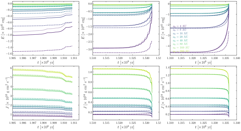
Examples of the evolution with time of the total energy are shown in the top panels of Fig. 13, specifically for simulations with 2, and 3 M⊙. More negative values represent higher binding energy configurations. Cases with values closer to zero represent simulations with less binding energy. The figure shows results for simulations including accretion from Paper I (solid lines), standard BHL accretion (dashed lines), and those without this effect (dotted lines). During most of the evolution of the symbiotic systems the energy is conserved at constant values, but it is only affected towards the end of the simulations, particularly during the TPAGB phase.
As previously discussed, simulations that exclude the accretion effect experience orbital expansion, producing a reduction in total energy due to mass lost from the system. This effect is particularly pronounced in systems with smaller initial orbital separations. Overall, models that incorporate accretion exhibit similar behaviour. The difference between models with and without accretion regarding energy is more notorious in the simulations of star and less prominent as the donor mass increases.
On the other hand, the total angular momentum is defined as
| (10) |
where denotes the position vector with respect to the centre of mass for each stellar component in the system.
Examples of the time evolution of the total angular momentum magnitude are shown in the bottom panels of Fig. 13. Similar to the evolution of , the total angular momentum remains largely unchanged throughout most of the simulation. However, noticeable variations occur during the TPAGB phase. The bottom panels of Fig. 13 reveal that all simulations (with and without accretion) exhibit a reduction in total angular momentum, but this reduction becomes significant only at the very end of the TPAGB phase. Although the orbital separation increases during most of the TPAGB phase (which would normally increase ), the mass lost by the system counteracts this effect, maintaining a relatively constant . A significant decrease in is observed only when the donor star undergoes its highest mass-loss rate during the final thermal pulse. It can be seen that simulations with accretion undergo less angular momentum loss than their counterparts without accretion. Models with small initial orbital separations including the standard BHL accretion scheme present an increase of in the final times of the evolution of a and 3 M⊙ stellar evolution, which is easily attributed to the excessive increase of in the last thermal pulses.
We also assesses the evolution of the eccentricity in the simulations. It was found that all simulations including any type of accretion remained virtually circular, with eccentricity values close to zero. Models without any type of accretion increase their eccentricity, particularly those with the most extended initial orbital configurations. For example, simulations with M⊙ resulted in binary configurations with . In the case of simulations with M⊙, models without accretion reached eccentricity values as large as 0.05.

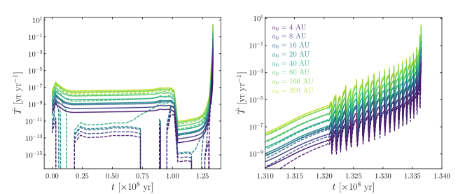
Finally, we assessed the orbital period decay by calculating the time derivate of the orbital period in our calculations, that is, . Fig. 14 illustrates the cases of and 3 M⊙ in the top and bottom panels, respectively. Depending on , the models produce a range of values of several orders of magnitude (left panels). Models including the wind accretion from Paper I (solid lines) behave very similar to simulations without accretion (dotted lines), as also illustrated by the orbital parameters evolution ( and ) of Fig. 4–7. Given the large mass accretion efficiency of models including the standard BHL scheme, there are periods of time where the orbits remain unchanged, thus, is virtually zero.
For comparison, we note that Chen et al. (2018) estimated a narrow range of values around yr yr-1 for their binary simulations that included wind accretion using the standard BHL formalism, which means that those systems are expanding their orbits, leading to less interacting binary systems. Understandably, their hydrodynamical simulations do not cover a larger evolving time of the modelled binary system. That range is achieved in our simulations during the TPAGB phase, but steadily increases reflecting the behaviour. Chen et al. (2018) found that their simulations with more compact binary systems, evolving through WRLOF, resulted in negative values. Consistently, our wind accretion simulations always resulted in .
5 Summary and concluding remarks
For decades, numerical simulations found that the standard implementation of the BHL wind accretion model for binary systems did not produce reliable results for the case where the stellar wind velocity was smaller than the orbital velocity of the accretor . A situation that is of outmost importance for symbiotic systems. The standard BHL scheme predicts non-physical mass accretion efficiencies larger than 1 for . Recently, Tejeda & Toalá (2024) (Paper I) proposed a geometric correction to the standard implementation of the BHL model for accreting binaries and found a better agreement between their analytical predictions and numerical simulations.
In this paper, we studied the impact of the wind accretion model of Paper I for the case of evolving symbiotic systems. We modelled 48 different symbiotic systems, each consisting of a WD with an initial mass of or 1.0 M⊙ and a Solar-like star with an initial mass of , 2, and 3 M⊙. The stars were placed in initially circular orbits with separations ranging from 4 to 200 AU. The evolution of the Solar-like stars was computed using the stellar evolution code mesa, and the orbital evolution of the systems was calculated making use of the N-body package rebound. For each configuration, we conducted three types of simulations: accretion using the modified model from Paper I, accretion using the standard BHL model, and no accretion.
Our main findings are summarized as follows:
-
•
The wide range of masses and orbital configurations modelled highlights distinct evolutionary paths. The adopted accretion prescription significantly affects the final destiny of the modelled symbiotic system. None of the simulations including the wind accretion from Paper I reached the Chandrasekhar limit (1.4 M⊙). This means that for this model to produce recurrent nova (e.g., T CrB) and type Ia supernova events in symbiotic systems, the accreting WD should start with an initial mass in the range known for ultra-massive WDs. This means, that the WD should be the descendent of a massive ( M⊙) progenitor. On the other hand, compact systems ( AU) modelled with the standard BHL scheme evolve ultimately taking the accreting WDs to this mass limit for the two adopted masses of the accretor. This discrepancy suggests that binary simulations and population synthesis studies relying on the BHL approximation may require revision, even in cases where arbitrary efficiency factors are adopted.
-
•
Simulations including the wind accretion from Paper I generally agree with binary and orbital properties of a number of observed symbiotic systems. The accretion properties of well-characterised symbiotic binaries, such as R Aqr and Y Gem, are nicely reproduced by the wind accretion scheme of Paper I. The nova recurrence time of R Aqr is estimated to be a few times 106 yr.
-
•
Simulations predict that accretors can transition back and forth through different recurrence nova times, and even between the three main accretion regimes (e.g., recurrence nova, steady burning, and giant envelope). Models that do not end in type Ia supernova events end up in the giant envelope accreting regime, given that the last thermal pulses from the donor star exhibit extreme events of mass loss.
-
•
The models produce bolometric luminosities consistent with optical and X-ray observations of symbiotic systems, supporting the reliability of the accretion scheme used in our simulation to match observed systems.
-
•
The total energy and angular momentum of modelled systems remain nearly constant during the RGB phase, with significant changes only occurring during the TPAGB phase. These changes are configuration-dependent and emphasize the influence of mass loss and accretion dynamics on system evolution.
-
•
Symbiotic systems with accretion maintain nearly circular orbits throughout their evolution, contrasting with systems without accretion, which develop increased eccentricities during the TPAGB phase. We confirm that wind accreting binaries exhibit , but the orbital period variation increase reflecting the evolution of from each stellar evolution model.
This study demonstrates the critical role of the adopted accretion prescription in shaping the evolution of symbiotic systems and highlights the limitations of standard BHL-based models. The results also emphasize the importance of wind accretion dynamics in reproducing observed systems, offering new insights into the progenitors and long-term evolution of symbiotic binaries. The next step will be to study the accretion scheme defined in Paper I but for the more complex interactions unveiled by eccentric cases (R. F. Maldonado et al. in prep.).
Acknowledgements
R.F.M. thanks UNAM DGAPA (Mexico) and SECIHTI (Mexico) for postdoc fellowships. J.A.T. and J.B.R.-G. acknowledge support from the UNAM PAPIIT project IN102324. This work has made extensive use of NASA’s Astrophysics Data System.
DATA AVAILABILITY
The model results underlying this article will be shared on reasonable request to the corresponding author.
References
- Alcolea et al. (2023) Alcolea, J., Mikolajewska, J., Gómez-Garrido, M., et al. 2023, Highlights on Spanish Astrophysics XI, 190
- Andrews et al. (2024) Andrews, J. J., Bavera, S. S., Briel, M., et al. 2024, arXiv:2411.02376
- Beers & Christlieb (2005) Beers, T. C. & Christlieb, N. 2005, ARA&A, 43, 531
- Bidelman & Keenan (1951) Bidelman, W. P. & Keenan, P. C. 1951, ApJ, 114, 473
- Blöcker (1995) Bloecker, T. 1995, A&A, 297, 727
- Bode (2010) Bode, M. F. 2010, Astronomische Nachrichten, 331, 160
- Boffin (2015) Boffin, H. M. J. 2015, Astrophysics and Space Science Library, 413, 153
- Bondi (1952) Bondi, H. 1952, MNRAS, 112, 195
- Bondi & Hoyle (1944) Bondi, H. & Hoyle, F. 1944, MNRAS, 104, 273
- Boneva & Yankova (2021) Boneva, D. & Yankova, K. 2021, The 20.5th Cambridge Workshop on Cool Stars, Stellar Systems, and the Sun (CS20.5), 328
- Boshkayev et al. (2016) Boshkayev, K. A., Rueda, J. A., Zhami, B. A., et al. 2016, International Journal of Modern Physics Conference Series, 41, 1660129
- Camisassa et al. (2019) Camisassa, M. E., Althaus, L. G., Córsico, A. H., et al. 2019, A&A, 625, A87
- Chen et al. (2018) Chen, Z., Blackman, E. G., Nordhaus, J., et al. 2018, MNRAS, 473, 747
- Chomiuk et al. (2021) Chomiuk, L., Metzger, B. D., & Shen, K. J. 2021, ARA&A, 59, 391
- Curd et al. (2017) Curd, B., Gianninas, A., Bell, K. J., et al. 2017, MNRAS, 468, 239
- García-Berro et al. (2012) García-Berro, E., Lorén-Aguilar, P., Aznar-Siguán, G., et al. 2012, ApJ, 749, 25
- García-Berro et al. (1997) García-Berro, E., Ritossa, C., & Iben, I. 1997, ApJ, 485, 765
- Gromadzki et al. (2006) Gromadzki, M., et al. 2006, Acta Astron., 56, 97
- Guerrero et al. (2024a) Guerrero, M. A., Vasquez-Torres, D. A., Rodríguez-González, J. B., et al. 2024, arXiv:2411.14270
- Guerrero et al. (2024b) Guerrero, M. A., Montez, R., Ortiz, R., et al. 2024, A&A, 689, A62
- Hachisu et al. (1996) Hachisu, I., Kato, M., & Nomoto, K. 1996, ApJ, 470, L97. doi:10.1086/310303
- Hansen et al. (2016) Hansen, T. T., Andersen, J., Nordström, B., et al. 2016, A&A, 588, A3
- Hermes et al. (2013) Hermes, J. J., Kepler, S. O., Castanheira, B. G., et al. 2013, ApJ, 771, L2
- Hillman & Kashi (2021) Hillman, Y. & Kashi, A. 2021, MNRAS, 501, 201
- Hoyle & Lyttleton (1939) Hoyle, F. & Lyttleton, R. A. 1939, Proceedings of the Cambridge Philosophical Society, 35, 405
- Huarte-Espinosa et al. (2013) Huarte-Espinosa, M., Carroll-Nellenback, J., Nordhaus, J., et al. 2013, MNRAS, 433, 295
- Hurley et al. (2002) Hurley, J. R., Tout, C. A., & Pols, O. R. 2002, MNRAS, 329, 897
- Izzard et al. (2009) Izzard, R. G., Glebbeek, E., Stancliffe, R. J., et al. 2009, A&A, 508, 1359
- Jermyn et al. (2023) Jermyn, A. S., Bauer, E. B., Schwab, J., et al., 2023, ApJS, 265, 15
- Karinkuzhi et al. (2024) Karinkuzhi, D., Mukhopadhyay, B., Wickramasinghe, D., et al. 2024, MNRAS, 529, 4577
- Kenyon & Truran (1983) Kenyon, S. J. & Truran, J. W. 1983, ApJ, 273, 280
- Leedjarv et al. (1994) Leedjarv, L., Mikolajewski, M., & Tomov, T. 1994, A&A, 287, 543
- Li et al. (2023) Li, Z., Chen, X., Ge, H., et al. 2023, A&A, 669, A82
- Lima et al. (2024) Lima, I. J., Luna, G. J. M., Mukai, K., et al. 2024, A&A, 689, A86
- Liu et al. (2017) Liu, Z.-W., Stancliffe, R. J., Abate, C., et al. 2017, ApJ, 846, 117. doi:10.3847/1538-4357/aa8622
- Luna et al. (2018) Luna, G. J. M., Mukai, K., Sokoloski, J. L., et al. 2018, A&A, 616, A53
- Luna et al. (2013) Luna, G. J. M., Sokoloski, J. L., Mukai, K., et al. 2013, A&A, 559, A6
- Malfait et al. (2024) Malfait, J., Siess, L., Esseldeurs, M., et al. 2024, A&A, 691, A84
- Marchev & Zamanov (2024) Marchev, V. D. & Zamanov, R. K. 2024, Bulgarian Astronomical Journal, 40, 85
- Merc et al. (2024) Merc, J., Beck, P. G., Mathur, S., et al. 2024, A&A, 683, A84
- Merc et al. (2019) Merc, J., Gális, R., & Wolf, M. 2019, Research Notes of the American Astronomical Society, 3, 28
- Mukai (2017) Mukai, K. 2017, PASP, 129, 062001
- Nagae et al. (2004) Nagae, T., Oka, K., Matsuda, T., et al. 2004, A&A, 419, 335
- Nomoto et al. (2007) Nomoto, K., Saio, H., Kato, M., et al. 2007, ApJ, 663, 1269
- Osborn et al. (2024) Osborn, Z., Karakas, A. I., Kemp, A. J., et al. 2024, arXiv:2412.01025
- Pasquini et al. (2023) Pasquini, L., Pala, A. F., Salaris, M., et al. 2023, MNRAS, 522, 3710
- Paxton et al. (2019) Paxton, B., Smolec, R., Schwab, J., et al. 2019, ApJS, 243, 10
- Paxton et al. (2018) Paxton, B., Schwab, J., Bauer, E. B., et al. 2018, ApJS, 234, 34
- Paxton et al. (2015) Paxton, B., Marchant, P., Schwab, J., et al. 2015, ApJS, 220, 15
- Paxton et al. (2013) Paxton, B., Cantiello, M., Arras, P., et al. 2013, ApJS, 208, 4
- Paxton et al. (2011) Paxton, B., Bildsten, L., Dotter, A., et al. 2011, ApJS, 192, 3
- Pringle (1981) Pringle, J. E. 1981, ARA&A, 19, 137
- Pujol et al. (2023) Pujol, A., Luna, G. J. M., Mukai, K., et al. 2023, A&A, 670, A32
- Ramstedt et al. (2020) Ramstedt, S., Vlemmings, W. H. T., Doan, L., et al. 2020, A&A, 640, A133
- Ramstedt et al. (2018) Ramstedt, S., Mohamed, S., Olander, T., et al. 2018, A&A, 616, A61
- Reimers (1975) Reimers, D. 1975, Memoires of the Societe Royale des Sciences de Liege, 8, 369
- Rein & Spiegel (2015) Rein, H. & Spiegel, D. S. 2015, MNRAS, 446, 1424.
- Rein & Liu (2012) Rein, H. & Liu, S.-F. 2012, A&A, 537, A128.
- Richards et al. (2024) Richards, S., Eldridge, J., Ghodla, S., et al. 2024, arXiv:2411.03000
- Robinson et al. (1994) Robinson, K., Bode, M. F., Skopal, A., et al. 1994, MNRAS, 269, 1
- Saladino & Pols (2019) Saladino, M. I. & Pols, O. R. 2019, A&A, 629, A103
- Saladino et al. (2019) Saladino, M. I., Pols, O. R., & Abate, C. 2019, A&A, 626, A68
- Schaefer (2023) Schaefer, B. E. 2023, Journal for the History of Astronomy, 54, 436
- Shakura & Sunyaev (1973) Shakura, N. I. & Sunyaev, R. A. 1973, A&A, 24, 337
- Shara et al. (2018) Shara, M. M., Prialnik, D., Hillman, Y., et al. 2018, ApJ, 860, 110. doi:10.3847/1538-4357/aabfbd
- Shen & Bildsten (2007) Shen, K. J. & Bildsten, L. 2007, ApJ, 660, 1444. doi:10.1086/513457
- Sokoloski et al. (2001) Sokoloski, J. L., Bildsten, L., & Ho, W. C. G. 2001, MNRAS, 326, 553
- Stanishev et al. (2004) Stanishev, V., Zamanov, R., Tomov, N., et al. 2004, A&A, 415, 609
- Starrfield & Sparks (1987) Starrfield, S. & Sparks, W. M. 1987, Ap&SS, 131, 379
- Tejeda & Toalá (2024) Tejeda, E. & Toalá, J. A. 2024, arXiv:2411.01755
- Theuns et al. (1996) Theuns, T., Boffin, H. M. J., & Jorissen, A. 1996, MNRAS, 280, 1264
- Toalá et al. (2024) Toalá, J. A., González-Martín, O., Sacchi, A., et al. 2024, MNRAS, 532, 1421
- Toalá et al. (2023) Toalá, J. A., González-Martín, O., Karovska, M., et al. 2023, MNRAS, 522, 6102
- Vathachira et al. (2024) Vathachira, I. B., Hillman, Y., & Kashi, A. 2024, MNRAS, 527, 4806
- Vasquez-Torres et al. (2024) Vasquez-Torres, D. A., Toalá, J. A., Sacchi, A., et al. 2024, MNRAS, 535, 2724
- Vennes & Kawka (2008) Vennes, S. & Kawka, A. 2008, MNRAS, 389, 1367
- Verbena et al. (2011) Verbena, J. L., Schröder, K.-P., & Wachter, A. 2011, MNRAS, 415, 2270
- Wolf et al. (2013) Wolf, W. M., Bildsten, L., Brooks, J., et al. 2013, ApJ, 777, 136
- Zamanov et al. (2024) Zamanov, R. K., Stoyanov, K. A., Marchev, V., et al. 2024, Astronomische Nachrichten, 345, e20240036
- Zhekov & Tomov (2019) Zhekov, S. A. & Tomov, T. V. 2019, MNRAS, 489, 2930
Appendix A Observation Symbiotic Systems
Table 3 lists the properties of symbiotic systems as listed in the New Online Database of Symbiotic Variables222https://sirrah.troja.mff.cuni.cz/~merc/nodsv/ (Merc et al., 2019). It lists the object name, masses of the stellar components ( and ), the binary period (), their estimated orbital separation (), the orbital velocity (), the dimensionless mass ratio as defined by Eq. (4), the dimensionless velocity parameter defined by Eq. (5) and the estimated mass accretion efficiency obtained from Eq. (2).
| Object | ||||||||
|---|---|---|---|---|---|---|---|---|
| [M⊙] | [M⊙] | [yr] | (AU) | [km s-1] | ||||
| Cet | 2.00 | 0.65 | 497.90 | 87.3 | 5.2 | 0.25 | 1.35 | |
| AE Ara | 2.00 | 0.51 | 2.00 | 2.2 | 32.2 | 0.20 | 0.47 | |
| AE Cir | 1.10 | 1.00 | 0.94 | 1.2 | 39.1 | 0.48 | 0.38 | |
| AG Dra | 1.20 | 0.50 | 1.51 | 1.6 | 31.1 | 0.29 | 0.48 | |
| AG Peg | 2.60 | 0.65 | 2.23 | 2.5 | 33.8 | 0.20 | 0.44 | |
| AR Pav | 2.00 | 0.75 | 1.65 | 2.0 | 35.4 | 0.27 | 0.42 | |
| AX Per | 3.00 | 0.60 | 1.86 | 2.3 | 37.2 | 0.17 | 0.40 | |
| BF Cyg | 1.50 | 0.40 | 2.07 | 2.0 | 29.0 | 0.21 | 0.52 | |
| BX Mon | 3.70 | 0.55 | 3.78 | 3.9 | 31.0 | 0.13 | 0.48 | |
| CH Cyg | 2.20 | 0.56 | 15.58 | 8.8 | 16.8 | 0.20 | 0.89 | |
| CI Cyg | 2.40 | 0.50 | 2.34 | 2.5 | 32.1 | 0.17 | 0.47 | |
| CQ Dra | 5.00 | 0.85 | 4.66 | 5.1 | 32.2 | 0.15 | 0.47 | |
| EG And | 1.46 | 0.40 | 1.32 | 1.5 | 33.5 | 0.22 | 0.45 | |
| ER Del | 3.00 | 0.70 | 5.72 | 5.0 | 25.8 | 0.19 | 0.58 | |
| FG Ser | 1.70 | 0.60 | 1.78 | 1.9 | 32.5 | 0.26 | 0.46 | |
| FN Sgr | 1.50 | 0.70 | 1.55 | 1.7 | 33.6 | 0.32 | 0.45 | |
| HD 330036 | 4.46 | 0.54 | 4.59 | 4.8 | 30.7 | 0.11 | 0.49 | |
| Hen 3-461 | 1.50 | 0.88 | 6.22 | 4.5 | 21.7 | 0.37 | 0.69 | |
| IV Vir | 0.90 | 0.42 | 0.77 | 0.9 | 35.7 | 0.32 | 0.42 | |
| KX TrA | 1.00 | 0.41 | 3.31 | 2.5 | 22.4 | 0.29 | 0.67 | |
| LT Del | 1.00 | 0.57 | 1.24 | 1.4 | 31.9 | 0.36 | 0.47 | |
| PU Vul | 1.00 | 0.50 | 13.42 | 6.5 | 14.4 | 0.33 | 1.04 | |
| R Aqr | 1.00 | 0.70 | 42.40 | 14.6 | 10.2 | 0.41 | 1.47 | |
| RW Hya | 1.60 | 0.48 | 1.01 | 1.3 | 38.0 | 0.23 | 0.39 | |
| St 2-22 | 2.80 | 0.80 | 2.51 | 2.9 | 33.6 | 0.22 | 0.45 | |
| SY Mus | 1.30 | 0.43 | 1.71 | 1.7 | 29.9 | 0.25 | 0.50 | |
| T CrB | 2.10 | 1.30 | 0.62 | 1.0 | 46.8 | 0.38 | 0.32 | |
| TX CVn | 3.50 | 0.40 | 0.55 | 1.1 | 57.4 | 0.10 | 0.26 | |
| V443 Her | 2.50 | 0.42 | 1.64 | 2.0 | 36.2 | 0.14 | 0.42 | |
| V455 Sco | 1.10 | 0.60 | 3.85 | 3.0 | 22.7 | 0.35 | 0.66 | |
| V471 Per | 2.30 | 0.80 | 17.00 | 9.4 | 16.4 | 0.26 | 0.92 | |
| V694 Mon | 1.00 | 0.90 | 5.28 | 3.8 | 21.2 | 0.47 | 0.71 | |
| V745 Sco | 1.00 | 1.38 | 1.40 | 1.7 | 35.6 | 0.57 | 0.42 | |
| V934 Her | 1.60 | 1.35 | 12.02 | 7.6 | 18.7 | 0.46 | 0.80 | |
| V1261 Ori | 1.65 | 0.55 | 1.75 | 1.9 | 32.2 | 0.25 | 0.47 | |
| V1329 Cyg | 2.10 | 0.70 | 2.62 | 2.7 | 30.5 | 0.25 | 0.49 | |
| V3890 Sgr | 1.05 | 1.35 | 2.05 | 2.2 | 31.5 | 0.56 | 0.48 | |
| Z And | 2.00 | 0.65 | 2.08 | 2.3 | 32.4 | 0.25 | 0.46 |