The Hydrostatic Mass of A478: Discrepant Results From Chandra, NuSTAR, and XMM-Newton

Cicely Potter Department of Physics & Astronomy, The University of Utah, 115 South 1400 East, Salt Lake City, UT 84112, USA Ayşegül Tümer Kavli Institute for Astrophysics and Space Research, Massachusetts Institute of Technology, 77 Massachusetts Avenue, Cambridge, MA 02139, USA Department of Physics & Astronomy, The University of Utah, 115 South 1400 East, Salt Lake City, UT 84112, USA Qian H. S. Wang Department of Astronomy, University of Maryland, College Park, MD 20742, USA Daniel R. Wik Department of Physics & Astronomy, The University of Utah, 115 South 1400 East, Salt Lake City, UT 84112, USA Ben J. Maughan H. H. Wills Physics Laboratory, University of Bristol, Tyndall Ave, Bristol BS8 1TL, UK Gerrit Schellenberger Center for Astrophysics, Harvard & Smithsonian, 60 Garden Street, Cambridge, MA 02138, USA

Abstract

Galaxy clusters are the most recently formed and most massive, gravitationally bound structures in the universe. The number of galaxy clusters formed is highly dependent on cosmological parameters, such as the dark matter density, $\sigma_{8}$ , and $\Omega_{m}$ . The number density is a function of the cluster mass, which can be estimated from the density and temperature profiles of the intracluster medium (ICM) under the assumption of hydrostatic equilibrium. The temperature of the plasma, hence its mass, is calculated from the X-ray spectra. However, effective area calibration uncertainties in the soft band result in significantly different temperature measurements from various space-based X-ray telescopes. NuSTAR is potentially less susceptible to these issues than Chandra and XMM-Newton, having larger effective area, particularly at higher energies, enabling high precision temperature measurements. In this work, we present analyses of Chandra, NuSTAR, and XMM-Newton data of Abell 478 to investigate the nature of this calibration discrepancy. We find that NuSTAR temperatures are on average $\sim$ 11% lower than that of Chandra, and XMM-Newton temperatures are on average $\sim$ 5% lower than that of NuSTAR. This results in a NuSTAR mass at $r_{2500,Chandra}$ of $M_{2500,NuSTAR}=3.39^{+0.07}_{-0.07}\times 10^{14}$ $M_{\odot}$ , which is $\sim$ 10% lower than that of $M_{2500,Chandra}$ and $\sim$ 4% higher than $M_{2500,XMM-Newton}$ .

X-rays: galaxies: clusters — galaxies: clusters: individual (A478)

1 introduction

Galaxy clusters form hierarchically from smaller, virialized structures at the peaks of the initial matter density fluctuations of the universe. Thus galaxy cluster number density is strongly dependent on the matter density of the universe, $\Omega_{m}$ , and the amplitude of the power spectrum, $\sigma_{8}$ , as well as the evolution of dark energy. The number density is a function of the cluster mass, meaning cluster mass can be used to constrain cosmological parameters (for example, Vikhlinin (2010), Burenin & Vikhlinin (2012), Bartalucci et al. (2018), Ettori et al. (2019), Ferragamo et al. (2021)).

Cluster mass can be calculated from the density and temperature profiles of the intracluster medium (ICM) under the assumption of hydrostatic equilibrium. These hydrostatic cluster mass measurements require a bias factor to be consistent with the best-fit Planck base- $\Lambda$ CDM cosmology as measured by cosmic microwave background anisotropies. While the bias factor of $(1-b)=0.62\pm 0.03$ found by Planck Collaboration et al. (2021) is within 1 $\sigma$ of weak lensing measurements, it is at the lower end.

X-ray spectra are ideal for measuring temperature; these temperature measurements, however, critically depend on the broadband calibration of a telescope’s effective area, or collecting area as a function of energy. The effective area will be less than the geometric area of the mirrors due to factors such as the quantum efficiency, vignetting, molecular contamination, and optical blocking filter transmission. Different X-ray telescopes report different temperatures for the same clusters, resulting in the masses differing by $\sim$ 10 $\%$ . This is suspected to be a calibration issue.

For a large sample of bright, nearby galaxy clusters Schellenberger et al. (2015) find that, at a cluster temperature of 10 keV, temperatures measured by the XMM-Newton European Photon Imaging Camera silicon pn-junction CCD (EPIC-PN) are on average $23\%$ lower than temperatures measured by Chandra Advanced CCD Imaging Spectrometer (ACIS). This is due to the effective area calibration uncertainties, mainly in the 0.7–2 keV band, between XMM-Newton and Chandra that have been revealed through the model-independent stacked residuals ratios (see also Nevalainen et al. (2010) and Kettula et al. (2013)). The difference between Chandra and XMM-Newton increases with cluster temperature, thus hotter clusters are ideal for investigating this difference further, and NuSTAR, with its harder response, is able to measure hotter temperatures more precisely.

XMM-Newton EPIC detectors MOS1, MOS2, and PN show disagreement as well, where systematically lower temperatures are measured with PN. When comparing the hard and soft band temperatures of one instrument, Schellenberger et al. (2015) found that Chandra ACIS temperatures are consistent with each other, while XMM-Newton EPIC are not. However, depending on the level of multiphase gas along the line of sight, a perfectly calibrated instrument is expected to show some level of deviation between the soft and hard band temperatures. Recent corrections to the effective areas of all three of XMM-Newton’s EPIC cameras were made with the intent to bring them into better agreement with NuSTAR¹¹1https://xmmweb.esac.esa.int/docs/documents/CAL-SRN-0388-1-4.pdf. These corrections only apply to the 3.0–12.0 keV band and are found to be successful in improving agreement between EPIC-PN and NuSTAR’s Focal Plane Modules A and B (FPMA and FPMB).

NuSTAR is potentially less susceptible to calibration issues than XMM-Newton and Chandra, having greater sensitivity at higher energies, where the effective area is relatively constant and the exponential turnover of the bremsstrahlung continuum is more prominent given its bandpass for hotter clusters. The exponential turnover provides the most constraining power on temperature in low resolution spectra. In a recent NuSTAR effective area calibration update, stray light observations of the Crab Nebula were used, allowing a more accurate measurement of the vignetting function; stray light observations bypass the optics, thus avoiding any degeneracy with the multilayer insulation and Be window. In addition to effective area changes, these updates bring FPMA and FPMB flux into better agreement with each other, increase the measured flux by $5$ – $15\%$ (depending on off-axis angle), and make more accurate high energy and off-axis angle corrections Madsen et al. (2021). Wallbank et al. (2022) find that, for a sample of 8 galaxy clusters, NuSTAR temperatures are $\sim$ 10% and $\sim$ 15% lower than Chandra temperatures in the broad and hard bands respectively.

Abell 478 (A478) is a nearby (z = 0.0856), massive, relaxed, cool-core galaxy cluster with $r_{2500,Chandra}$ ²²2 $r_{\Delta}$ corresponds to the radius of a point on a sphere whose density equals $\Delta$ times the critical density of the background universe, $\rho_{c}$ (z), at the cluster redshift where $\Delta$ is the density contrast. $=589\pm 14$ kpc and $r_{500,Chandra}\sim 1514$ kpc.

Vikhlinin et al. (2006b) measure the spectroscopic temperature of A478 with Chandra data to be $7.95\pm 0.14$ keV, and Arnaud et al. (2005) measure it with XMM-Newton data to be $7.05\pm 0.12$ keV. This results in masses of 4.12 $\pm$ 0.26 $\times$ $10^{14}$ $M_{\odot}$ and 3.12 $\pm$ 0.31 $\times$ $10^{14}$ $M_{\odot}$ at $r_{2500}$ for Chandra and XMM-Newton, respectively. This is a difference of 11% between spectroscopic temperatures and 26% between masses. This disagreement is partially due to differences in analysis, such as the regions the spectra are extracted from or the choice of spectral models and their parameters. For example, some of the difference may have since been resolved with the Chandra CALDB update from version 3 to 4. While some differences are unavoidable due to inherent instrument properties, we attempt to provide analyses of the data from Chandra, NuSTAR, and XMM-Newton that differ in method as little as possible.

Throughout this paper, we assume $\Lambda$ CDM cosmology with H₀ = 71 km s^-1 Mpc^-1, $\Omega_{M}$ = 0.3, $\Omega_{\Lambda}$ = 0.7. According to these assumptions, at the cluster redshift, a projected intracluster distance of 100 kpc corresponds to an angular separation of $\sim$ 61 $\arcsec$ . All uncertainties are quoted at the 68% confidence levels unless otherwise stated.

The paper is organized as follows: description of the data, data reduction processes, and background assessment for Chandra, NuSTAR, and XMM-Newton are presented in Section 2. The methods used for the analyses of the cluster data and the results are presented in Section 3. In Section 4, we discuss our findings.

2 Data Reduction

Observation Log
		Date	RA	Dec	Exposure
	Observation ID	(yyyy-mm-dd)	(J2000)	(J2000)	(ks)	PI
Chandra	1669 (ACIS-S)	2001-01-27	63.36	10.44	42.9	Murray
	6102 (ACIS-I)	2004-09-13	63.37	10.49	10.5	Allen
NuSTAR	70660002002	2020-09-29	63.35	10.45	207.9 (FPM(A+B))	Wik
	70660002004	2020-09-29	63.35	10.45	260.7 (FPM(A+B))	Wik
XMM-Newton	109880101	2002-02-15	63.38	10.47	57.7 (MOS1)/94.2 (MOS2)/62.6 (PN)	Brinkman

Table 1: Observation log of the Chandra, NuSTAR, and XMM-Newton data used for analysis. The exposure shown is that of the observations before filtering and data reduction.

Refer to caption — Figure 1: The raw (Left) and background subtracted, exposure corrected (Right) 0.8–2 keV counts images of the Chandra observations. The spectrum was extracted from each of the annuli shown; these spectra were fit to get the observed temperature profile. The excluded regions are the point sources manually selected from a 0.5–4.0 keV image. The radii of the annuli are 30″, 68″, 101″, 152″, 228″, 342″, and 513″.

2.1 Chandra

In this work we used two sets of Chandra data consisting of one ACIS-S and one ACIS-I pointing (see Table 1). For the Chandra data reduction, we use HEASoft³³3https://heasarc.gsfc.nasa.gov/lheasoft/ version 6.30.1, CIAO⁴⁴4https://cxc.cfa.harvard.edu/ciao/ version 4.12, and CALDB version 4.7.6. The python code acisgenie⁵⁵5https://gitlab.com/qwq/acisgenie was used to generate scripts to run the standard CIAO data filtering commands.

First, any linear streaks caused by flaws in readout were removed with destreak. Bad pixels both from the framestore and the observation itself, including afterglow and hot pixels, were saved in a file with acis_build_badpix. The event file information was then updated with acis_process_events. A histogram of the duration vs. pointing and roll offsets was created with asphist, and this was later used to create the auxiliary response files. Periods of anomalously high or low counts between 2.3–7.3 keV were removed with lc_clean. Point sources were excluded manually from a 0.5–4.0 keV image with circular regions a minimum of 25 $\arcsec$ in radius created in SAOImageDS9⁶⁶6https://sites.google.com/cfa.harvard.edu/saoimageds9 (see Fig. 1). Any visible point sources not excluded were determined to be negligible. The final GTI for observation 1669 is $\sim$ 42 ks for the front-illuminated chips and $\sim$ 40 for the back-illuminated chips, and the final GTI for observation 6102 is $\sim$ 7 ks. ACIS blank sky backgrounds that match the observation were obtained using acis_backgrnd_lookup. These backgrounds were then tailored to match the data by also being filtered for bad pixels, aligned with the observation, and scaled by the 9.5–12.0 keV counts in the observation event file. A script written by Maxim Markevitch, called make_readout_bg⁷⁷7https://cxc.cfa.harvard.edu/contrib/maxim/make_readout_bg, was used to create a model background file to correct for other ACIS readout artifacts. The raw and cleaned Chandra images are shown in Fig. 1.

The spectrum was extracted with the CHAV⁸⁸8http://hea-www.harvard.edu/~alexey/CHAV/ tool runextrspec. The data reduction, background creation, and spectral extraction steps we followed are described in more detail by Wang et al. (2016), however, we fit the spectra jointly in Xspec rather than combining them as done by Wang et al. (2016).

2.2 NuSTAR

The two NuSTAR observations used in this work include both FPMA and FPMB spectra (Table 1). A user-defined GTI was created by removing flares with lcfilter⁹⁹9https://github.com/danielrwik/reduc. This command creates light curves from the A and B modules separately, binned by 100 seconds. Bins with count rates greater than the local distribution were identified manually and excluded, resulting in a $\sim$ 2–3 $\sigma$ cut. The final GTIs were $\sim$ 98 and $\sim$ 122 ks for 70660002002 and 70660002004, respectively. This process is described in more detail by Rojas Bolivar et al. (2021).

For the NuSTAR data reduction, we use HEASoft version 6.28, NuSTARDAS¹⁰¹⁰10https://heasarc.gsfc.nasa.gov/docs/nustar/analysis/ version 2.0.0, and CALDB index version 20200912. The background spectra were extracted via nuproducts from square regions a little smaller than the chips, with an elliptical exclusion region to remove cluster emission (see Fig. 2). These background spectra were fit using nuskybgd¹¹¹¹11https://github.com/NuSTAR/nuskybgd; this code models the solar, focused cosmic x-ray, aperture, and internal background components, as well as an APEC component for the residual cluster emission (Wik et al., 2014). The APEC model is sufficient to account for all cluster emission not excluded by the elliptical exclusion region. The temperature, abundance, and normalization parameters of the APEC model were left free to vary but tied across FPMA and FPMB. The redshift was fixed at 0.0856 (Xu et al., 2022). A constant component was included to account for the cross-calibration of the A and B modules, where the parameter value was fixed at 1 for FPMA and free to vary for FPMB. The final background fits for observation 70660002004 are shown in Fig. 3. Following the background fit, the spectra were extracted from the annuli via using nuproducts with bkgextract=no because we use the backgrounds fit with nuskybgd. The point source regions excluded were the same as for Chandra. The resulting background subtracted, exposure-corrected image can be seen in Fig. 4.

2.3 XMM-Newton

The center of A478 was observed by XMM-Newton in 2002 for 126.6 ks (OBSID 0109880101; first reported in Pointecouteau et al., 2004). A shorter offset pointing also covers part of the cluster, but we only analyze data from the longer central pointing. Images and spectra are extracted following the Extended Source Analysis Software (XMM–ESAS)¹²¹²12https://heasarc.gsfc.nasa.gov/docs/xmm/xmmhp_xmmesas.html package, included as part of SAS version 20.0.0, with a calibration analysis date of 2022-05-13. We used the standard data filtering and processing techniques as part of the analysis procedure (e.g., Snowden et al., 2008). The clean exposure times for the three EPIC instruments amounted to 55.7 ks, 94.2 ks, and 62.6 ks for Metal Oxide Semi-conductors 1 and 2 (MOS1 and 2) and PN, respectively. In addition to the annular regions described above for Chandra NuSTAR and XMM-Newton spectra extraction, spectra from an outer annular region extending out to 13′ were also extracted in order to better constrain foreground Galactic emission and absorption, which were modeled and simultaneously fit with the annular regions following Snowden et al. (2008).

We also make use of two corrections to the effective area calibration, which are applied in the call to the SAS task arfgen by setting two keywords: applyabsfluxcorr=yes¹³¹³13https://xmmweb.esac.esa.int/docs/documents/CAL-TN-0230-1-3.pdf and applyxcaladjusment=yes¹⁴¹⁴14https://xmmweb.esac.esa.int/docs/documents/CAL-TN-0018.pdf. The former correction increases the $E>4$ keV EPIC effective area by a few percent, which brings the observed spectral indices of bright point sources observed simultaneously by XMM-Newton and NuSTAR into agreement; although empirically determined only for EPIC-PN, the correction is applied to all three detectors for consistency. Despite the name, the applyabsfluxcorr keyword does not make any corrections to the flux. The effect this correction has on the XMM-Newton temperatures can be seen in Appendix C. The latter correction further increases the hard band MOS effective areas to bring their measurements into better agreement with those of the PN. These corrections bring XMM-Newton detector spectra into a better agreement with each other and with NuSTAR spectra, although they do not necessarily ensure a more accurate calibration. However, we note that simultaneous, absorbed single temperature fits to all annuli are better fit when these corrections are applied, and the residual soft proton contribution is also better constrained. The raw and cleaned XMM-Newton images are shown in Fig. 5.

3 Analysis and Results

3.1 Temperature and Density Profile Extraction

The Chandra, NuSTAR, and XMM-Newton spectra were extracted from circular and annular regions to create a radial temperature profile. The chosen regions consist of a central circle of radius 30″ and 5 concentric annuli starting at 30″, all centered at 63.3546^∘, 10.4655^∘. The outer radius of each annulus was 1.5x the inner radius, though the inner two annuli later had to be combined to ensure each region was large enough to accurately correct for crosstalk due to NuSTAR’s point spread function (PSF); the code used to correct for crosstalk, described in section 3.2, requires regions to have a radius $\geq 30\arcsec$ . This logarithmic spacing was chosen to maintain high signal to noise. Because they have a larger field of view than NuSTAR, one extra annulus was included for both Chandra and XMM-Newton (see Figures 1 and 5).

All of the spectra were fit using Xspec¹⁵¹⁵15https://heasarc.gsfc.nasa.gov/docs/xanadu/xspec/. The Chandra and NuSTAR spectra channels were grouped with grppha¹⁶¹⁶16https://heasarc.gsfc.nasa.gov/docs/journal/grppha4.html to a minimum of 3 counts, and the C statistic was used to fit them. While the C statistic is more appropriate, it is also more computationally exspensive. Because of this, the XMM-Newton spectra were grouped to a minimum of 30 counts, and the chi-square statistic was used. The choice of statistic has a negligible effect on the resulting best-fit temperatures according to tests, and thus this choice should not affect any results.

The APEC and TBABS models were used to fit all spectra. The Chandra spectra of both obsids were jointly fit between 0.8–9 keV, and all parameters besides the APEC norm were tied. The NuSTAR FPMA/B spectra of both obsids were fit between 3–15 keV, and the XMM-Newton MOS1/2 and PN spectra were fit between 0.4–11 keV.

The Wilms (XSpec table wilm; Wilms et al., 2000) abundances were used for all fits; using the Anders and Grevesse (angr; Anders & Grevesse, 1989) abundances instead resulted in temperature differences of around $1\%$ at most for NuSTAR and around $5\%$ for both Chandra and XMM-Newton. The Wilms table was used because it agrees better with HI measurements, as well as being generally better for fitting Galactic absorption (Wilms et al. (2000); Willingale et al. (2013)). While NuSTAR abundances are estimated based on the Fe complex alone, Chandra and XMM-Newton measurements are also impacted by unresolved lines at lower energies. However, some of the flux at these lower energies is also affected by the amount of line-of-sight absorption ( $N_{H}$ ); if the $N_{H}$ is over- or underestimated, it will affect the abundance estimates as well. This degeneracy can cause differences in both abundance and $N_{H}$ measurements between the different telescopes and can be particularly sensitive to the accuracy of the calibration at low energies.

In this work, the XMM-Newton abundances are, excluding the outermost region, an average of $\sim$ 10% lower than the Chandra abundances. In the outermost region, the XMM-Newton abundance is $\sim$ 66% larger than the Chandra abundance. The average difference between the Chandra and XMM-Newton abundances is $\sim$ 0.1 $Z_{\odot}$ . Changing the Chandra abundances by this amount results in a difference of $\sim$ 0.02 keV in the center and $\sim$ 0.13 keV in the outskirts. These differences are smaller than the $1\sigma$ confidence on the temperatures. Similarly, changing the XMM-Newton abundances by $\sim$ 0.1 $Z_{\odot}$ results in temperature differences of $\sim$ 0.01 keV in the center, and $\sim$ 0.10 keV in the outskirts, which are on the order of the $1\sigma$ errors (see Table 2). The NuSTAR abundances are an average of $\sim$ 38% lower than the Chandra abundances. This is a difference of $\sim$ 0.2 $Z_{\odot}$ . Changing the NuSTAR abundances by this amount results in a difference of $\sim$ 0.05 keV in the center and $\sim$ 0.1 keV in the outskirts, which is a little larger than the $1\sigma$ errors.

The $N_{H}$ along the line of sight of A478 changes with cluster radius and is larger than the radio value of $1.5\times 10^{21}$ from the HI4PI survey (HI4PI Collaboration et al., 2016). Vikhlinin et al. (2005) find that the best-fit Chandra $N_{H}$ changes linearly with radius from $3.09\pm 0.09\times 10^{21}$ cm^-2 at the center to $2.70\pm 0.06\times 10^{21}$ cm^-2 at $4\arcmin$ . Pointecouteau et al. (2004) find that the best-fit XMM-Newton $N_{H}$ also changes with radius from $3.00\pm 0.10\times 10^{21}$ cm^-2 at $0.14\arcmin$ to $2.41\pm 0.08\times 10^{21}$ cm^-2 at $4.54\arcmin$ . These profiles agree in the center but progress to a difference of $\sim$ 11 $\%$ around $4\arcmin$ . In this work, $N_{H}$ was left free for each region individually for both Chandra and XMM-Newton. This results in the XMM-Newton $N_{H}$ values being an average of $\sim$ 13% lower, with the maximum difference in the outermost region, where the XMM-Newton $N_{H}$ is $\sim$ 26% lower. This is an average difference between the Chandra and XMM-Newton $N_{H}$ of $\sim 5\times 10^{20}$ cm^-2 (see Table 2). Changing the Chandra or XMM-Newton $N_{H}$ values by this amount results in a temperature difference of $\sim$ 0.4 keV in the center and up to $\sim$ 1 keV in the outskirts for both telescopes. Setting $N_{H}$ at the radio value found by HI4PI Collaboration et al. (2016) more than doubles the temperatures for both telescopes as well. The temperature profile that results from fixing the Chandra $N_{H}$ to the XMM-Newton best-fit values, as well as the XMM-Newton spectra with $N_{H}$ fixed to the Chandra best fit values can be seen in Appendix D. NuSTAR is less sensitive to absorption (Tümer et al., 2023); in the central region, the inclusion of $N_{H}$ fixed to the best-fit Chandra value decreases the temperature by $\sim$ 1% compared to a fit without it.

A detailed investigation into these differences is beyond the scope of this work, which considers absorption and abundance to be nuisance parameters even though they could bias temperature estimates from Chandra and XMM-Newton.

The APEC norms also differ between telescopes. Since the norm depends on the electron and proton densities, differences in the norms imply differences in flux. The NuSTAR fluxes are an average of $\sim$ 9% and $\sim$ 4% lower than the Chandra ACIS-S and ACIS-I fluxes respectively, excluding NuSTAR’s outermost region (Chandra’s second to last region), where the NuSTAR flux is $\sim$ 40% higher than the ACIS-S flux, and $\sim$ 3% higher than the ACIS-I flux. The two outermost Chandra regions contain very little of the ACIS-S observation, so this is expected. The XMM-Newton (MOS1) fluxes are an average of $\sim$ 24% lower than the ACIS-S Chandra fluxes, excluding the two outermost regions, where the XMM-Newton fluxes are $\sim$ 13% and $\sim$ 65% larger, respectively. The XMM-Newton fluxes are an average of $\sim$ 25% lower than the ACIS-I Chandra fluxes. The XMM-Newton fluxes are also an average of $\sim$ 18% lower than the NuSTAR fluxes. Thus, there is tension not only in the temperatures but in the fluxes as well.

The redshift for NuSTAR was fixed at $0.0856$ , and a gain offset was added and free to fit. The resulting gain is $-0.102^{+7e-6}_{-0.001}$ keV. This adjustment is needed to eliminate systematic residuals in the Fe K complex while obtaining the known redshift of the cluster; similar gain adjustments of $\sim$ 0.1 keV are required when fitting other clusters, suggesting a small miscalibration at lower energies (Rojas Bolivar et al., 2021). The Chandra redshift was free to vary in each region to account for any differences in gain between them due to spanning across both the ACIS-S and ACIS-I observations. The resulting best-fit values are an average of $\sim$ 4 $\%$ higher than the accepted value of 0.0856 (Xu et al., 2022), excluding the second to last region, which has a best-fit value $\sim$ 10 $\%$ lower. Fixing the redshift in this region at 0.0856 increased the temperature by 0.02 keV, or $\sim$ 0.3 $\%$ , which is less than the 1 $\sigma$ temperature uncertainty of -0.31,+0.17 keV. The redshift was free to vary but tied across regions for XMM-Newton to account for gain. The resulting best-fit value is $\sim$ 5 $\%$ lower than the accepted value.

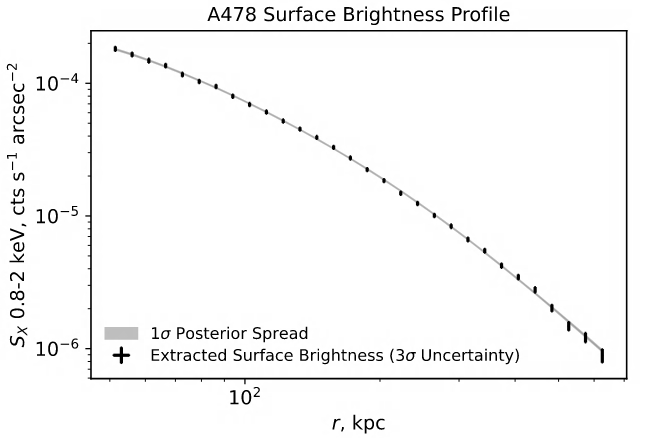
The projected surface brightness was extracted by calculating the count mean in the background subtracted, exposure corrected (flux) mosaic Chandra image in logarithmic radial bins. The image is masked with the excluded point source regions. The uncertainty is calculated assuming Poisson statistics. This surface brightness profile was used for determining the Chandra, NuSTAR, and XMM-Newton mass estimates because Chandra has higher spatial resolution than both NuSTAR and XMM-Newton. This profile was fit using a double beta model and emissivity table, as discussed in section 3.6.

3.2 Crosstalk Correction

NuSTAR has a larger PSF than both Chandra and XMM-Newton. Photons from different parts of the gas are mixed and need to be disentangled. To correct for this crosstalk between the annular regions, nucrossarf¹⁷¹⁷17https://github.com/danielrwik/nucrossarf was used; this code creates new response matrix files (RMF), ancillary response files (ARF), and background files based on the shape of NuSTAR’s PSF. These new files were used to jointly fit the annular spectra in Xspec. For the source image, or the image that gives nucrossarf the actual distribution of photons, we used a point-source masked and filled XMM-Newton image in the 2.35–7.2 keV band because the NuSTAR image has already been smoothed by the PSF. We do not use the Chandra image because, while Chandra has the greatest spatial resolution, the Chandra image has more artifacts from combining ACIS-S and ACIS-I observations. Additionally, XMM-Newton has a greater effective area in the hard band, thus it more closely resembles NuSTAR images. How the nucrossarf code disentangles the crosstalk is explained in detail by Tümer et al. (2023).

XMM-Newton’s PSF is also larger than Chandra’s. However, with it being smaller than NuSTAR’s PSF, and with the regions being as large as they are, we do not correct XMM-Newton’s PSF.

3.3 NuSTAR Temperature Map

A temperature map of the NuSTAR observation 70660002002 was made by first separating the spectrum into narrow energy bands of 3–5 keV, 6–10 keV, and 10–20 keV. A circle was drawn at every 5th pixel, which had a minimum radius of 5 pixels. Then the radius of the circle was increased until 1000 counts were reached to ensure $<$ 10% precision measurements. This was done for the raw count, background, and exposure images for all 3 bands.

The exposure corrected, background subtracted counts in each of these bands together form a rough spectrum that is fit in Xspec for each circle. The center pixel of each circle is then assigned the resulting best-fit temperature. Then the temperature is interpolated between each of the central pixels in order to make an image. The NuSTAR temperature map made with this method can be seen in Fig. 6.

The temperature map shows that the core is cooler, and temperature generally increases with radius. Multiple hot spots can be seen within the annular regions. Those that do not appear to correspond to point sources could be areas of hot gas in the cluster, and thus were not excluded in the spectral extraction.

To derive a radial temperature profile from the temperature map, we create concentric annular regions and find the average or median temperature from all the measurements inside the region. This profile can then be compared to the temperature profile derived by directly fitting spectra in annular regions using nuproducts response files (Fig. 7), to evaluate the accuracy of the temperatures in the map. We find that the profile is in good agreement with the nuproducts-derived profile, except that the profile from the map is systematically lower by $\sim$ 0.25 keV. This indicates a small systematic difference between how the temperatures are estimated in the two cases—likely resulting from the much more coarse-grained nature of the temperature map fits—but confirms the general consistency of the temperature map measurements and that from direct spectral fitting. However, in both cases the measured temperatures suffer from spatial mixing due to the PSF; the nucrossarf-derived temperatures are the best temperature estimates, since they account for this effect, and are what we use for the NuSTAR temperature profile and mass estimates.

3.4 Comparing Temperature Profiles

Vikhlinin et al. (2005) compare the observed temperature profile from Chandra and XMM-Newton of A478, in addition to several other clusters. For most clusters, the XMM-Newton temperature profile agrees with the Chandra profile after a +10% renormalization to account for cross-calibration. For A478 however, the profiles are significantly different within the central 4′; the XMM-Newton profile increases gradually before becoming relatively constant, whereas the Chandra profile increases more rapidly, peaks, and begins to decrease. This is attributed to an incomplete correction of XMM-Newton’s PSF and the complex temperature structure in the cluster center.

We do not correct for XMM-Newton’s PSF in this work, but NuSTAR’s PSF has been corrected with nucrossarf. The scattering from the PSF smoothed out the profile, making the inner region appear hotter and the outer regions appear cooler. After correction, the inner region is much cooler, and the outer regions are hotter. While this creates a more rapid increase to the peak, the nucrossarf profile is still in better agreement with XMM-Newton than Chandra (see Fig. 7 and Table 2). The NuSTAR temperatures are around 11% lower than Chandra on average, with the largest difference in the 3rd region, where NuSTAR is 18% cooler than Chandra. The largest difference between the NuSTAR and XMM-Newton profiles is in the 4th region, where the XMM-Newton temperature is $\sim$ 10% lower than the NuSTAR temperature. The XMM-Newton temperatures are lower than the NuSTAR temperatures by $\sim$ 5% on average. For a comparison to temperature profiles found in other works, see Appendix E.

Xspec Fit Parameters
	Radii	kT	Z	N_H	norm
	(arcsec)	(keV)	( $Z_{\odot}$ )	(10²² cm^-2)	( $10^{-2}$ )	z
Chandra	0 $-$ 30	$4.71^{+0.05}_{-0.05}$	$0.71^{+0.02}_{-0.01}$	$0.457^{+0.005}_{-0.003}$	$1.641^{+0.005}_{-0.008}$	$0.088^{+0.001}_{-0.001}$
	30 $-$ 68	$6.54^{+0.06}_{-0.11}$	$0.64^{+0.02}_{-0.03}$	$0.441^{+0.005}_{-0.003}$	$1.964^{+0.005}_{-0.009}$	$0.086^{+0.001}_{-0.001}$
	68 $-$ 101	$7.57^{+0.13}_{-0.16}$	$0.54^{+0.03}_{-0.04}$	$0.426^{+0.006}_{-0.004}$	$1.218^{+0.006}_{-0.008}$	$0.086^{+0.001}_{-0.001}$
	101 $-$ 152	$7.65^{+0.15}_{-0.19}$	$0.65^{+0.02}_{-0.08}$	$0.409^{+0.006}_{-0.004}$	$1.136^{+0.006}_{-0.005}$	$0.084^{+0.001}_{-0.001}$
	152 $-$ 228	$7.82^{+0.14}_{-0.26}$	$0.43^{+0.03}_{-0.06}$	$0.410^{+0.005}_{-0.005}$	$1.042^{+0.004}_{-0.006}$	$0.086^{+0.002}_{-0.002}$
	228 $-$ 342	$7.21^{+0.17}_{-0.31}$	$0.48^{+0.06}_{-0.05}$	$0.375^{+0.010}_{-0.007}$	$0.497^{+0.003}_{-0.006}$	$0.077^{+0.006}_{-0.002}$
	342 $-$ 513	$8.29^{+0.80}_{-0.85}$	$0.41^{+0.21}_{-0.22}$	$0.275^{+0.034}_{-0.022}$	$0.124^{+0.005}_{-0.005}$	$0.087^{+0.008}_{-0.010}$
nucrossarf	0 $-$ 30	$4.52^{+0.02}_{-0.02}$	$0.43^{+0.01}_{-0.01}$	0.457^∗	$1.648^{+0.010}_{-0.010}$	0.0856^†
	30 $-$ 68	$5.77^{+0.02}_{-0.02}$	$0.48^{+0.01}_{-0.01}$	0.441^∗	$2.192^{+0.008}_{-0.009}$	-
	68 $-$ 101	$6.21^{+0.04}_{-0.04}$	$0.29^{+0.02}_{-0.02}$	0.426^∗	$1.336^{+0.008}_{-0.009}$	-
	101 $-$ 152	$6.87^{+0.05}_{-0.05}$	$0.44^{+0.02}_{-0.02}$	0.409^∗	$1.163^{+0.006}_{-0.007}$	-
	152 $-$ 228	$6.77^{+0.05}_{-0.05}$	$0.30^{+0.02}_{-0.02}$	0.410^∗	$1.014^{+0.006}_{-0.007}$	-
	228 $-$ 342	$6.78^{+0.06}_{-0.06}$	$0.22^{+0.02}_{-0.02}$	0.375^∗	$0.793^{+0.006}_{-0.006}$	-
XMM-Newton	0 $-$ 30	$4.53^{+0.03}_{-0.03}$	$0.68^{+0.01}_{-0.01}$	$0.406^{+0.002}_{-0.002}$	$1.262^{+0.003}_{-0.003}$	$0.0816^{+0.0002}_{-0.0002}$ ^‡
	30 $-$ 68	$5.65^{+0.04}_{-0.04}$	$0.56^{+0.01}_{-0.01}$	$0.390^{+0.002}_{-0.002}$	$1.836^{+0.003}_{-0.003}$	-
	68 $-$ 101	$5.91^{+0.06}_{-0.06}$	$0.54^{+0.02}_{-0.02}$	$0.383^{+0.003}_{-0.003}$	$0.953^{+0.001}_{-0.001}$	-
	101 $-$ 152	$6.23^{+0.06}_{-0.06}$	$0.44^{+0.02}_{-0.02}$	$0.376^{+0.002}_{-0.002}$	$1.030^{+0.004}_{-0.003}$	-
	152 $-$ 228	$6.43^{+0.07}_{-0.08}$	$0.42^{+0.02}_{-0.02}$	$0.355^{+0.002}_{-0.002}$	$0.817^{+0.002}_{-0.002}$	-
	228 $-$ 342	$6.40^{+0.11}_{-0.10}$	$0.44^{+0.03}_{-0.03}$	$0.327^{+0.003}_{-0.003}$	$0.618^{+0.003}_{-0.003}$	-
	342 $-$ 516	$6.03^{+0.42}_{-0.36}$	$0.68^{+0.09}_{-0.09}$	$0.236^{+0.036}_{-0.034}$	$0.222^{+0.002}_{-0.002}$	-

^*^*footnotetext: Fixed to the Chandra best-fit hydrogen column density values.

^†^†footnotetext: Fixed to 0.0856 and tied across regions.

^‡^‡footnotetext: Free to fit and tied across regions.

Table 2: Spectral fit results for all annuli of Chandra, NuSTAR, and XMM-Newton.

3.5 Temperature Weighting

When converting to a projected temperature profile model, the 3D temperature profile model was weighted based on detector sensitivity. The following weighting formula was used (Vikhlinin, 2006a):

\left<T\right>=\frac{\int_{V}c(T)\rho^{2}T^{1-\alpha}dV}{\int_{V}c(T)\rho^{2}T^{-\alpha}dV},

(1)

where $c(T)$ is the detector sensitivity to bremsstrahlung radiation and $\rho$ is the density profile. For $\rho$ we use the Chandra density profile, as given in Fig. 13. Simulations of NuSTAR spectra were done in Xspec with temperatures 4 & 5 keV, 4 & 6 keV, 4 & 7 keV, 5 & 6 keV, 5 & 7 keV, and 6 & 7 keV, where the lower temperature has a norm of $f_{min}$ , and the higher temperature has a norm of $1-f_{min}$ . These were saved and then fit to single temperature models in the range 3–15 keV. The results of these fits are shown in Fig. 8. The best-fit value of $\alpha$ for NuSTAR was found to be $-0.35$ . The best value for Chandra and XMM-Newton is found by Vikhlinin (2006a) to be $0.75$ .

3.6 Fitting the Temperature and Density Profiles

The 3D temperature profile model used is that also used by Vikhlinin et al. (2006b), and is as follows:

T_{3D}(r)=\frac{T_{0}(r/r_{t})^{-a}}{\left[1+(r/r_{t})^{b}\right]^{c/b}}\times T_{cool},

(2)

where the $T_{cool}$ component (Allen et al., 2001) is described by Vikhlinin et al. (2006b) as

T_{cool}=\frac{(r/r_{c})^{a_{c}}+T_{min}/T_{0}}{(r/r_{c})^{a_{c}}+1}.

(3)

Thus the model has nine parameters ( $T_{0}$ , $r_{t}$ , $a$ , $b$ , $c$ , $T_{min}$ , $r_{c}$ , $a_{c}$ ) to be fit. This 3D model cannot be fit directly to the observed temperature profile because the observed profile is actually a projection of the cluster temperature. After being weighted based on the weighting formula (see section 3.5), the 3D temperature model is integrated along the line of sight to a truncation radius of 3500 kpc; this is the projected model (blue) in Figures 9, 10, and 11. The projected profile is then fit to the observed temperature profile and binned based on the inner and outer radii of the regions.

The effect of $T_{cool}$ on the profile is focused mainly in the center, which has less of an effect on the final mass than the overall profile. The $T_{cool}$ parameters were fixed to the best-fit values found by Vikhlinin et al. (2006b) for one fit, and left free to vary with the rest of the parameters for another. The rest of the parameters were left free for all fits, since the observed profiles of this work differ from the observed Chandra profile found by Vikhlinin et al. (2006b) (see Section 3.4). The resulting mass at $r_{2500,Chandra}$ with fixed $T_{cool}$ parameters was $\sim$ 1% lower for Chandra, $\sim$ 2% lower for NuSTAR, and $\sim$ 7% lower for XMM-Newton.

The 3D density model is a double- $\beta$ model (Hudson et al., 2010):

n(r)=\left[n_{1}^{2}(1+(r/r_{1})^{2})^{-3\beta_{1}}+n_{2}^{2}(1+(r/r_{2})^{2})^{-3\beta_{2}}\right]^{1/2}.

(4)

An emissivity table was used to convert this density model to a surface brightness model. This table was constructed by first extracting the Chandra spectrum in a circular region with a 3 $\arcmin$ radius centered on the cluster. After modeling the spectrum with the APEC model in Xspec, the APEC norm was set to 1, and the model count rate was recorded for each point in a matrix of temperature and abundance values. Thus, the resulting density fit subsumed the APEC norm and has to be normalized after the fit. Because the surface brightness profile comes from the Chandra mosaic image, including both the ACIS-S and ACIS-I observations, only the Chandra emissivity table was calculated. In future work, surface brightness and emissivity tables from XMM-Newton and NuSTAR can be derived and used as well. Corrections for PSF cross-talk for both observatories must be applied to these processes. Because the focus of this work is on the impact of different temperature measurements between instruments, the use of only Chandra surface brightness and emissivity profiles should not significantly affect our results.

The emissivity table is converted to a function via interpolation. The function is then given the abundance and temperature model parameters to calculate the emissivity as a function of radius. This profile is then multiplied by the density model squared, then multiplied by 2 and integrated along the line of sight to a truncation radius of 3500 kpc; the resulting profile is fit to the observed surface brightness profile (see Fig. 12). Since the emissivity function depends on the temperature model fit, the density model fit will depend on the temperature model fit as well. Additionally, the temperature weighting, and thus the temperature model fit, depends on the density model fit. Thus, these models were iteratively fit with chi-squared minimization.

3.7 Markov Chain Monte Carlo For Confidence Intervals

The python package emcee¹⁸¹⁸18https://emcee.readthedocs.io/en/v2.2.1/ was used to run a Markov chain Monte Carlo (MCMC) simulation on the temperature and density profile parameters. MCMC is used to sample posterior probability distribution functions (pdf) by comparing pairs of points; this means that it is insensitive to pdf normalization, and does not need a full analytic description of the pdf (Hogg & Foreman-Mackey, 2018).

The log-likelihood function, or the function that determines whether a set of parameters is accepted or not, comes from the residuals of both temperature and surface brightness models:

-\frac{1}{2}\Sigma\left[\left(\frac{T-T_{model}}{T_{err}}\right)^{2}+\left(\frac{SB-SB_{model}}{SB_{err}}\right)^{2}\right]

(5)

The code was given the best-fit parameters as a starting point, and then it was given a step size for each parameter, the number of walkers (50), and the number of iterations (1000). Because of the small effect of the $T_{cool}(r)$ term, the $T_{min}$ , $r_{c}$ , and $a_{c}$ parameters were fixed at the best-fit values for each telescope while running the chain. The acceptance fraction, on average, was $\sim$ 0.23; this indicates that the chosen step size was appropriate, being close to 0.234, the ideal for high dimensional models (Hogg & Foreman-Mackey, 2018). Though the chain was not run for the recommended 50 times the integrated autocorrelation time, the walkers passed through the high probability areas of the parameter space many times, which indicates that the length of the chain was appropriate as well.

After the chain is run, it is flattened; all of the walker’s chains are appended to one single chain. The 16th and 84th quantiles are taken to be the lower and upper confidence intervals respectively. Since MCMC is not an optimizer, these samples are the spread around the resulting median model, rather than the optimized model. The resulting spread of the temperature profile models can be seen in Figures 9, 10, and 11. The spread in the surface brightness model can be seen in Figure 12. The median temperature and density model parameters are presented in Tables 3 and 4, respectively. The parameters can be slightly degenerate (as evidenced by the differing parameters from Chandra, XMM-Newton, and NuSTAR for the same density profile), so the confidence interval from MCMC is more helpful to view for the models as a whole, rather than for the parameters individually. However, the parameter confidence intervals are also given in Tables 3 and 4, and a corner plot of the Chandra MCMC simulations can be seen in Appendix F.

3D Temperature Model Parameters
	$T_{0}$	$r_{t}$				$T_{min}$	$r_{c}$
	(keV)	(kpc)	$a$	$b$	$c/b$	(keV)	(kpc)	$a_{c}$
Chandra:
Fixed $T_{cool}$	11.62	97.86	-0.24	5.00^∗	0.09	4.20	129.00	1.60
Free $T_{cool}$	8.0 ${}^{+0.2}_{-0.2}$	260 ${}^{+90}_{-60}$	-0.11 ${}^{+0.02}_{-0.02}$	4.5 ${}^{+0.3*}_{-0.4}$	0.05 ${}^{+0.02}_{-0.01}$	5.03	73.70	10.00
NuSTAR:
Fixed $T_{cool}$	9.29	44.38	-1.00	5.00^∗	0.22	4.20	129.00	1.60
Free $T_{cool}$	7.3 ${}^{+0.2}_{-0.2}$	310 ${}^{+50}_{-40}$	-0.22 ${}^{+0.01}_{-0.01}$	4.4 ${}^{+0.3*}_{-0.7}$	0.08 ${}^{+0.03}_{-0.02}$	1.32	32.55	10.00
XMM-Newton:
Fixed $T_{cool}$	9.03	46.97	-0.41	5.00^∗	0.11	4.20	129.00	1.60
Free $T_{cool}$	7.0 ${}^{+0.2}_{-0.2}$	630 ${}^{+200}_{-55}$	-0.12 ${}^{+0.01}_{-0.01}$	4.4 ${}^{+0.3*}_{-0.8}$	0.12 ${}^{+0.10}_{-0.05}$	3.29	28.37	10.00

^*^*footnotetext: 5.00 is the maximum value allowed by the fit.

Table 3: The 3D temperature model parameters for Chandra, NuSTAR, and XMM-Newton both when the

T_{cool}

parameters are fixed to those given in Vikhlinin et al. (2006b), and when they are free to be fit. The fixed

T_{cool}

parameters are found with a chi-squared fit. The free

T_{cool}

parameters were first found with a chi-squared fit, then run through MCMC simulations with

T_{min}

r_{c}

, and

a_{c}

held constant; excluding these last 3 parameters, the values presented here are the median values from the MCMC simulations. Confidence intervals are thus not given for the last 3 parameters of the free

T_{cool}

fit or the fixed

T_{cool}

fit, since they were not simulated via MCMC. Note that it is more informative to view the confidence intervals on the models as a whole, which can be seen in Figures 9, 10, 11, and 12.

Density Model Parameters
	$n_{1}$	$r_{1}$		$n_{2}$	$r_{2}$
	$(cm^{-3})$	(kpc)	$\beta_{1}$	$(cm^{-3})$	(kpc)	$\beta_{2}$
Chandra:
Fixed $T_{cool}$	$1.39\times 10^{-4}$	59.73	0.67	$3.42\times 10^{-5}$	166.82	0.69
Free $T_{cool}$	$1.41^{+0.08}_{-0.07}\times 10^{-4}$	59 ${}^{+4}_{-4}$	0.67 ${}^{+0.06}_{-0.04}$	$3.5^{+0.5}_{-0.4}\times 10^{-5}$	160 ${}^{+10}_{-10}$	0.68 ${}^{+0.02}_{-0.02}$
NuSTAR:
Fixed $T_{cool}$	$1.46\times 10^{-4}$	58.56	0.66	$3.38\times 10^{-5}$	166.74	0.68
Free $T_{cool}$	$1.48^{+0.06}_{-0.06}\times 10^{-4}$	56 ${}^{+3}_{-3}$	0.64 ${}^{+0.03}_{-0.03}$	$3.23^{+0.5}_{-0.4}\times 10^{-5}$	170 ${}^{+10}_{-10}$	0.69 ${}^{+0.03}_{-0.02}$
XMM-Newton:
Fixed $T_{cool}$	$1.40\times 10^{-4}$	60.10	0.67	$3.37\times 10^{-5}$	168.24	0.69
Free $T_{cool}$	$1.41^{+0.08}_{-0.07}\times 10^{-4}$	59 ${}^{+5}_{-4}$	0.67 ${}^{+0.05}_{-0.04}$	$3.5^{+0.5}_{-0.5}\times 10^{-5}$	160 ${}^{+10}_{-10}$	0.68 ${}^{+0.02}_{-0.02}$

Table 4: The density model parameters for Chandra, NuSTAR, and XMM-Newton both when the

T_{cool}

parameters are fixed to those given in Vikhlinin et al. (2006b), and when they are free to be fit. Though only the Chandra surface brightness profile is fit for the density model, the fit also depends on the temperature model fit, thus the density parameters are slightly different for each profile. The fixed

T_{cool}

parameters are found with a chi-squared fit. The free

T_{cool}

parameters were first found with a chi-squared fit, then run through MCMC simulations; thus, confidence intervals are only given for the free

T_{cool}

fits. Note that it is more informative to view the confidence intervals on the models as a whole, which can be seen in Figures 9, 10, 11, and 12.

3.8 Calculating Mass From Temperature and Density Profiles

Relaxed galaxy clusters are assumed to be in hydrostatic equilibrium (HSE), the condition where the gas pressure in the cluster is balanced with the gravitational force. From the HSE equation, the total mass can be estimated within radius $r$ (Vikhlinin et al., 2006b):

M_{HSE}(r)=-\frac{kT(r)r}{G\mu m_{p}}\left(\frac{d\mathrm{log}n(r)}{d\mathrm{log}r}+\frac{d\mathrm{log}T(r)}{d\mathrm{log}r}\right)\,,

(6)

where k, G, $\mu$ , and $m_{p}$ are the Boltzmann constant, gravitational constant, mean molecular weight, and the mass of a proton, respectively. Assuming the ICM is an ionized plasma, the mean molecular weight is 0.5954 (Vikhlinin et al., 2006b). The mass profile depends on radius, X-ray temperature as a function of radius, $T(r)$ , and density as a function of radius, $n(r)$ .

However, any sources of nonthermal pressure support, such as turbulence and bulk motions due to mergers, can result in an underestimate of hydrostatic mass. Pearce et al. (2019) state that nonthermal pressure is expected to contribute up to 30% of the total pressure. They simulate a sample consisting of 45 clusters in the mass range of $8\times 10^{13}<M_{500}\left[M_{\odot}\right]<2\times 10^{15}$ in various dynamical states to test the contribution of nonthermal pressure support. They apply a correction to the hydrostatic mass equation (6):

M_{corr}(r)=\frac{1}{1-\alpha}\left[M_{HSE}(r)-\frac{\alpha}{1-\alpha}\frac{kT(r)r}{G\mu m_{p}}\frac{d\mathrm{log}\alpha}{d\mathrm{log}r}\right]

(7)

where $\alpha$ is:

\alpha(r)=1-A\left(1+\mathrm{exp}\left[-\left(\frac{r/r_{500}}{B}\right)^{C}\right]\right)

(8)

and $A=0.45$ , $B=0.84$ , $C=1.63$ (Nelson et al., 2014), and $r_{500}$ is the radius at which the cluster has an overdensity of 500.

Ettori & Eckert (2021) calculate another model for nonthermal pressure support and apply it to the X-COP galaxy clusters. They find that the constraints on the ratio of nonthermal pressure to total pressure are between 0 and $\sim$ 20% at $r_{500}$ for all clusters in the sample except Abell 2319 at $\sim$ 54%; the contribution of nonthermal pressure support in Abell 2319 is expected to be higher because it is a merging cluster.

Since the contribution of nonthermal pressure support increases with mass, Eqn. 7 is an average solution. However, A478 is within the range of masses included in the simulations, so we have applied this correction in this work; the masses calculated with Eqn. 6 ( $M_{HSE}$ ) as well as those corrected for nonthermal pressure support ( $M_{corr}$ ) are reported in Table 5. We find that it results in masses around $13\%$ larger at $r_{2500,Chandra}$ than without nonthermal pressure support.

From the nonthermal pressure support corrected data we find $r_{2500,Chandra}=589\pm 14$ and $r_{500,Chandra}$ to be $\sim$ 1514 kpc, and use these values to calculate the masses from all three telescopes.

3.9 Mass Profiles

The resulting nonthermal pressure support corrected Chandra, XMM-Newton, and NuSTAR mass profiles are presented in Figure 14. As expected, the Chandra and NuSTAR masses differ by $\sim$ 10% at $r_{2500,Chandra}$ , while the difference between XMM-Newton and NuSTAR at $r_{2500,Chandra}$ is $\sim$ 4%; these differences are the same whether comparing $M_{HSE}$ or $M_{corr}$ .

The Chandra mass profile is largest due to having the hottest overall temperature. The Chandra 3D temperature model has the shallowest slope from 100 kpc to $\sim$ 350 kpc, which results in the mass increasing more slowly; this is why the Chandra mass profile comes closer to the NuSTAR mass profile before $\sim$ 350 kpc. The Chandra and NuSTAR 3D temperature profiles have a similar peak at $\sim$ 350 kpc, and a similar decreasing slope outside $\sim$ 350 kpc, resulting in their mass profiles having a similar slope outside $\sim$ 350 kpc. XMM-Newton has the lowest overall temperature, resulting in the smallest mass profile. However, XMM-Newton’s 3D temperature profile has a hotter core than NuSTAR’s, so the XMM-Newton mass profile starts at a higher mass than NuSTAR at 100 kpc. From 100 kpc to $\sim$ 350 kpc, XMM-Newton’s 3D temperature profile has a shallower slope than NuSTAR’s, resulting in XMM-Newton’s mass profile increasing more slowly; this causes the XMM-Newton mass profile to cross NuSTAR’s and become smaller. Then, from $\sim$ 350 kpc to $\sim$ 600 kpc XMM-Newton’s 3D temperature profile continues increasing while NuSTAR’s reaches its peak and begins decreasing. This causes the XMM-Newton mass profile to increase more quickly than the NuSTAR mass profile, once again crossing it, and end up just above the NuSTAR mass profile at $\sim$ 837 kpc.

The confidence intervals shown in Fig. 14 are the result of calculating the mass for each set of parameters simulated by the MCMC simulation, then calculating the 16th and 84th quantiles. The Chandra, NuSTAR, and XMM-Newton masses at $r_{2500,Chandra}$ and $r_{500,Chandra}$ are given in Table 5. Due to our largest profile ending around $\sim$ 837 kpc, $r_{500,Chandra}$ , as well as all masses calculated at this radius, are an extrapolation of our data and thus are not presented with confidence intervals. We compare to masses found in other works as well. Since each work measures the overdensities at different radii, these radii are also given in Table 5.

Mass of A478
		$M_{2500}$	$r_{2500}$	$M_{500}$	$r_{500}$
		( $10^{14}$ $M_{\odot}$ )	(kpc)	( $10^{14}$ $M_{\odot}$ )	(kpc)
$M_{HSE}$	Chandra	$3.28^{+0.10}_{-0.07}$	$589\pm 14^{*}$	8.00^†	$1514^{*}$
	NuSTAR	$2.96^{+0.06}_{-0.06}$	$589\pm 14^{*}$	7.17^†	$1514^{*}$
	XMM-Newton	$2.86^{+0.07}_{-0.07}$	$589\pm 14^{*}$	6.87^†	$1514^{*}$
$M_{corr}$	Chandra	$3.77^{+0.12}_{-0.09}$	$589\pm 14^{*}$	12.79^†	$1514^{*}$
	NuSTAR	$3.39^{+0.07}_{-0.07}$	$589\pm 14^{*}$	11.45^†	$1514^{*}$
	XMM-Newton	$3.28^{+0.08}_{-0.08}$	$589\pm 14^{*}$	10.98^†	$1514^{*}$
	Chandra (Vikhlinin et al., 2006b)	$4.12\pm 0.26$	$\sim 0.4r_{500}$	$7.68\pm 1.01$	$1337\pm 58$
	XMM-Newton (Arnaud et al., 2005)	$3.12\pm 0.31$	$\sim 0.3r_{200}^{\ddagger}$	$7.57\pm 1.11$	$1348\pm 64$
	Chandra (Mahdavi et al., 2007)	$4.9\pm 0.9$	$680\pm 70$	$9.9\pm 2.6$	$1500\pm 200$
	XMM-Newton (Mahdavi et al., 2007)	$3.3\pm 0.2$	$590\pm 20$	$8.2\pm 1.0$	$1400\pm 100$
	Chandra (Mantz et al., 2016)	$3.69\pm 0.15$	$620\pm 8$	-	-
	Chandra (Wulandari et al., 2019)	$2.0\pm 0.5$	$570\pm 80^{\S}$	-	-
	Sunyaev Z’eldovich Effect (Comis et al., 2011)	$2.8\pm 1.1$	$570\pm 80$	-	-

^*^*footnotetext: The masses of NuSTAR and XMM-Newton are calculated at

r_{2500,Chandra}

and

r_{500,Chandra}

as well, to make comparison as simple as possible.

^†^†footnotetext: The extracted temperature and surface brightness profiles only reach

\sim

250 kpc past

r_{2500,Chandra}

, thus the masses at

r_{500,Chandra}

are an extrapolation.

^‡^‡footnotetext: Arnaud et al. (2005) report

r_{200}=2060\pm 618

kpc.

^§^§footnotetext: Wulandari et al. (2019) adopt the value of

r_{2500}

found by Comis et al. (2011).

Table 5: The Chandra, NuSTAR, and XMM-Newton total masses found in this work at

r_{2500,Chandra}=589\pm 14

and

r_{500,Chandra}\sim 1514

kpc both calculated from the hydrostatic mass equation directly (

M_{HSE}

) and corrected for nonthermal pressure support (

M_{corr}

). Masses from other works are shown for reference; since each work calculates a different value for

r_{2500}

and

r_{500}

, these radii are given in the third and fifth columns, respectively. Additionally, the cosmology assumed in these works varies, resulting in varying values for the critical density,

\rho_{c}

(z), and thus differences in the relation between

r_{\Delta}

and

M_{\Delta}

. All uncertainties shown are

1\sigma

4 Discussion

We find that the temperature profile of A478 measured by NuSTAR is $\sim$ 11% cooler than the Chandra temperature profile on average. This results in the NuSTAR mass at $r_{2500,Chandra}$ being $\sim$ 10% lower than the Chandra mass, and $\sim$ 4% higher than the XMM-Newton mass. Wallbank et al. (2022) find that, for a sample of 8 galaxy clusters, NuSTAR temperatures are $\sim$ 10% and $\sim$ 15% lower than Chandra temperatures in the broad and hard bands, respectively. They discuss the effect the uncertainty in the background modeling might have on the temperatures and find that the signal-to-noise was high enough in their sample that the temperature fits were insensitive to the background modeling. They also find that, since the Chandra temperatures remain systematically higher than NuSTAR when limited to the hard band, this discrepancy is not due to any factors that affect soft band modeling, such as absorption along the line of sight and ACIS contamination.

The difference in the shape of the temperature profile of A478 between Chandra and XMM-Newton is explained by Vikhlinin et al. (2006b) to be an incomplete correction of XMM-Newton’s PSF. Though NuSTAR does have a larger PSF than both Chandra and XMM-Newton, this was corrected using the shape of the PSF to determine the scatter of emission from one annulus to another and creating ARFs to account for it. While we do not quantify any systematic effects of nucrossarf here, it does not appear to have any bias, as forthcoming work will show. Even after this correction, the NuSTAR profile is in better agreement with XMM-Newton than Chandra. Though XMM-Newton’s PSF is not corrected here, the annular regions are large enough that we believe the effect of it to be negligible.

Bandpass can affect temperature measurements; at softer energies, temperature is determined mainly by the power law-like slope of the bremsstrahlung spectrum, which can be biased by other sources of emission or mischaracterized background or absorption due to Galactic column density. In this work, the broad bands of each instrument were used to determine temperature; Chandra spectra were fit from 0.8–9 keV, XMM-Newton spectra from 0.4–11 keV, and NuSTAR spectra from 3–15 keV. Thus, NuSTAR is less susceptible to these issues than Chandra and XMM-Newton, being more sensitive to the exponential turnover of the bremsstrahlung spectrum, where temperature can be more accurately measured.

To extract the projected temperature profile, the ICM is assumed to be isothermal in each annulus, but this is not the case (see Fig. 6). Given that NuSTAR is more sensitive to higher energies than Chandra and XMM-Newton, and thus would be more sensitive to the higher temperature components of the gas, NuSTAR would be expected to measure higher temperatures than both Chandra and XMM-Newton. However, we find that the NuSTAR temperature profile for A478 is lower than Chandra and not much higher than XMM-Newton.

Sanderson et al. (2005) simulated multiphase gas with four temperature components (6, 6.5, 7.5, and 8 keV) using both the Chandra and XMM-Newton spectral responses and background spectra of A478. The simulations had a Galactic absorption of $2.7\times 10^{21}$ cm^-2 and an abundance of 0.3 Z_⊙. They used a single absorbed MEKAL model to fit the spectra with both the narrow (6.0–6.8 keV) and broad (0.7–7.0 keV) bands of both Chandra and XMM-Newton. They find that the fits do not show any significant disagreement between Chandra and XMM-Newton. With another set of simulations with two temperatures (5 and 12 keV) and different abundances, they find that when the hotter phase has a higher metallicity, the narrow band temperature increases for both Chandra and XMM-Newton, and a lower metallicity for the hotter phase decreases the narrow band temperature for both telescopes. Again, there is no significant disagreement between the Chandra and XMM-Newton temperatures. Thus, they conclude that the discrepancy between Chandra and XMM-Newton cannot be entirely attributed to nonisothermality in the ICM.

Similarly, Schellenberger et al. (2015) simulated spectra for Chandra ACIS-I and all three XMM-Newton instruments. The cold temperature components were 0.5, 1, and 2 keV, and the hot temperature component was varied from 3 to 10 keV. The hot component had a fixed abundance of 0.3 $Z_{\odot}$ , while the cold components had 0.3, 0.5, and 1 $Z_{\odot}$ , respectively. The spectra were fit with single temperature models, with the abundance free to vary. They find that when the cold temperature component is $\sim$ 2 keV, the fit is good, regardless of the amount of cold gas. The temperatures only begin to differ significantly when the cold component is $\sim$ 0.5 keV. Thus, they conclude that multiphase gas is not enough to explain the differences between the Chandra and XMM-Newton temperatures.

NuSTAR is also less sensitive to absorption than Chandra and XMM-Newton due to its lack of sensitivity below 3 keV (Rojas Bolivar et al., 2021), meaning the complicated absorption along the line of sight of A478 has less of an effect on temperature measurements. Tümer et al. (2023) find that leaving the $N_{H}$ parameter free for a global NuSTAR fit of CL 0217+70 results in unphysical behavior, demonstrating NuSTAR’s insensitivity to absorption.

The XMM-Newton temperature profile used by Arnaud et al. (2005) to find the mass of A478 is given by Pointecouteau et al. (2004). Their profile peaks around 3.66–4.54′ or $\sim$ 400 kpc and is 6.91 keV, which is around 0.5 keV hotter than found in this work. de Plaa et al. (2004) find an XMM-Newton profile that peaks around 2.0–3.0′ or $\sim$ 250 kpc at 6.76 keV, around 0.3 keV higher than ours. Sanderson et al. (2005) find a profile that also peaks around $\sim$ 250 kpc (123–175″), and their peak temperature is 7.06 keV, which is $\sim$ 0.6 keV higher than ours. Bourdin & Mazzotta (2007) measure their peak temperature of 7.5 keV around 3.5′or $\sim$ 340 kpc; this is closest to our peak radially, but a little over 1 keV hotter.

Our XMM-Newton temperature profile of A478 agrees fairly well with other recent works; though it is cooler than each of the profiles discussed here, the peak of the profiles line up radially. The cooler temperatures are likely due to the recent XMM-Newton calibration update, which brought it into better agreement with NuSTAR. This update included the addition of the applyabsfluxcorr keyword, which we make use of in this work. The effect this correction has on temperature can be seen in Appendix C. Our XMM-Newton temperature profile compared to other works can be seen in Appendix E.

Our Chandra temperature profile is cooler than found by Vikhlinin et al. (2005) by $\sim$ 1 keV, though their peak lines up with ours at around 250–300 kpc. Sanderson et al. (2005) also find a temperature profile that seems to peak around 175–250 $\arcsec$ or $\sim$ 300 kpc, at 8.12 keV, which is hotter than our peak by $\sim$ 0.3 keV. The peak temperature found by Mantz et al. (2016) is around 8 keV, thus $\sim$ 0.2 keV hotter than ours, and also appears to peak around 300 kpc. Thus our Chandra profile, while cooler than those found in other works, peaks at around the same radius and has the same general shape. Our Chandra profile compared to that of Sanderson et al. (2005) can be seen in Appendix E.

Differences in analysis such as how the data is reduced, which models are used to fit the spectra, and calibration updates will cause differences in measured temperature. The Chandra and XMM-Newton temperature profiles from this work compared to other works whose temperature profiles were given in tables can be seen in Appendix E.

Our final masses at $r_{2500,Chandra}$ and $r_{500,Chandra}$ are given in Table 5. We give the 68% confidence interval for the mass at $r_{2500}$ , but not for the extrapolated masses at $r_{500}$ since our data does not extend that far. We’ve included masses and the radii at which they’re measured from other works as well.

At $r_{2500,Chandra}$ our Chandra mass is $\sim$ 8% smaller than found by Vikhlinin et al. (2006b) at their measured $r_{2500}$ , which is expected since our temperature profile is cooler. Our Chandra mass at $r_{2500,Chandra}$ is also $\sim$ 23% smaller than found by Mahdavi et al. (2007), at their $r_{2500}$ who jointly fit X-ray, Sunyaev-Zel’dovich effect (SZE), and weak lensing data to calculate the mass. The Chandra mass at their $r_{2500}$ found by Mantz et al. (2016) is 2 $\%$ smaller than ours at $r_{2500,Chandra}$ , and the mass found by Wulandari et al. (2019), who adopt the value of $r_{2500}$ found by Comis et al. (2011), is $\sim$ 47% smaller than ours. Our XMM-Newton mass at $r_{2500,Chandra}$ is $\sim$ 5% larger than found by Arnaud et al. (2005) at their $r_{2500}$ , and $\sim$ 1% larger than found by Mahdavi et al. (2007) at their $r_{2500}$ . Our Chandra, XMM-Newton, and NuSTAR masses at $r_{2500,Chandra}$ are $\sim$ 34%, $\sim$ 17%, and $\sim$ 21% larger than the x-ray calibrated SZE mass at their $r_{2500}$ found by Comis et al. (2011) respectively.

Our NuSTAR mass at $r_{2500,Chandra}$ is smaller than all but one of Chandra masses presented (at their respective $r_{2500}$ ) by up to $\sim$ 31%; it is $\sim$ 41% larger than the Chandra mass found by Wulandari et al. (2019) at their $r_{2500}$ . Our NuSTAR mass at $r_{2500,Chandra}$ is $\sim$ 3 $\%$ larger than the XMM-Newton mass found by Mahdavi et al. (2007) at their $r_{2500}$ , and $\sim$ 9% larger than the XMM-Newton mass found by Arnaud et al. (2005) at their $r_{2500}$ .

Assuming NuSTAR is more accurate, cluster masses previously measured with Chandra could be $\sim$ 10% too large. The effect will be strongest on $\sigma_{8}$ , which is sensitive to the high cluster mass end of the mass function. With the HIFLUGCS sample of clusters, Schellenberger & Reiprich (2017) find that the smaller XMM-Newton masses result in a lower $\sigma_{8}$ than Chandra masses. The smaller NuSTAR masses found in this work would result in lower $\sigma_{8}$ values than the Chandra masses as well. These results, however, are based entirely on one cluster; Abell 478. This analysis will be repeated for three other clusters also recently observed with NuSTAR to determine whether this difference in mass is systematic or unique to this cluster.

This research was supported by the NASA grant 80NSSC21K0075. This research has made use of the NuSTAR Data Analysis Software (NuSTARDAS)¹⁹¹⁹19https://heasarc.gsfc.nasa.gov/docs/nustar/analysis/ jointly developed by the ASI Space Science Data Center (SSDC, Italy) and the California Institute of Technology (Caltech, USA). The data analysis software HEASoft²⁰²⁰20https://heasarc.gsfc.nasa.gov/lheasoft/, maintained by NASA’s HEASARC, was used in the analysis of both the Chandra and NuSTAR data, and the Chandra X-ray Center’s software package CIAO²¹²¹21https://cxc.cfa.harvard.edu/ciao/ was used in analyzing the Chandra data. XMM–ESAS²²²²22https://heasarc.gsfc.nasa.gov/docs/xmm/xmmhp_xmmesas.html, developed at Goddard Space Flight Center with cooperation with the XMM-Newton Science Operations Center, was used in the analysis of the XMM-Newton data. The data was obtained from the Chandra Data Archive, the XMM-Newton Science Archive, and the NuSTAR mission, which is led by the California Institute of Technology (Caltech, USA), managed by the Jet Propulsion Labratory, and funded by NASA. The MCMC tutorial “MCMC: A (very) Beginnner’s Guide,”²³²³23https://prappleizer.github.io/Tutorials/MCMC/MCMC_Tutorial.html written by Imad Pasha was extremely helpful for writing the MCMC code for confidence intervals.

References

Allen et al. (2001) Allen, S. W., Schmidt, R. W., & Fabian, A. C. 2001, MNRAS, 328, L37, doi: 10.1046/j.1365-8711.2001.05079.x
Anders & Grevesse (1989) Anders, E., & Grevesse, N. 1989, Geochim. Cosmochim. Acta, 53, 197, doi: 10.1016/0016-7037(89)90286-X
Arnaud (1996) Arnaud, K. A. 1996, in Astronomical Society of the Pacific Conference Series, Vol. 101, Astronomical Data Analysis Software and Systems V, ed. G. H. Jacoby & J. Barnes, 17
Arnaud et al. (2005) Arnaud, M., Pointecouteau, E., & Pratt, G. W. 2005, Astronomy & Astrophysics, 441, 893, doi: 10.1051/0004-6361:20052856
Bartalucci et al. (2018) Bartalucci, I., Arnaud, M., Pratt, G. W., & Le Brun, A. M. C. 2018, A&A, 617, A64, doi: 10.1051/0004-6361/201732458
Blanchard et al. (2018) Blanchard, A., Sakr, Z., & IliĆ, S. 2018, Cosmological cluster tension, arXiv, doi: 10.48550/ARXIV.1805.06976
Bourdin & Mazzotta (2007) Bourdin, H., & Mazzotta, P. 2007, Astronomy & Astrophysics, 479, 307, doi: 10.1051/0004-6361:20065758
Burenin & Vikhlinin (2012) Burenin, R. A., & Vikhlinin, A. A. 2012, Astronomy Letters, 38, 347, doi: 10.1134/S1063773712060011
Comis et al. (2011) Comis, B., de Petris, M., Conte, A., Lamagna, L., & de Gregori, S. 2011, MNRAS, 418, 1089, doi: 10.1111/j.1365-2966.2011.19562.x
de Plaa et al. (2004) de Plaa, J., Kaastra, J. S., Tamura, T., et al. 2004, Astronomy & Astrophysics, 423, 49, doi: 10.1051/0004-6361:20047170
Ettori & Eckert (2021) Ettori, S., & Eckert, D. 2021, Astronomy & Astrophysics, 657, L1, doi: 10.1051/0004-6361/202142638
Ettori et al. (2019) Ettori, S., Ghirardini, V., Eckert, D., et al. 2019, Astronomy & Astrophysics, 621, A39, doi: 10.1051/0004-6361/201833323
Ferragamo et al. (2021) Ferragamo, A., Barrena, R., Rubiño-Martín, J. A., et al. 2021, A&A, 655, A115, doi: 10.1051/0004-6361/202140382
Foreman-Mackey (2016) Foreman-Mackey, D. 2016, The Journal of Open Source Software, 1, 24, doi: 10.21105/joss.00024
Foreman-Mackey et al. (2013) Foreman-Mackey, D., Hogg, D. W., Lang, D., & Goodman, J. 2013, Publications of the Astronomical Society of the Pacific, 125, 306, doi: 10.1086/670067
Fruscione et al. (2006) Fruscione, A., McDowell, J. C., Allen, G. E., et al. 2006, in Society of Photo-Optical Instrumentation Engineers (SPIE) Conference Series, Vol. 6270, Society of Photo-Optical Instrumentation Engineers (SPIE) Conference Series, ed. D. R. Silva & R. E. Doxsey, 62701V, doi: 10.1117/12.671760
Gordon & Arnaud (2021) Gordon, C., & Arnaud, K. 2021, PyXspec: Python interface to XSPEC spectral-fitting program, Astrophysics Source Code Library, record ascl:2101.014. http://ascl.net/2101.014
HI4PI Collaboration et al. (2016) HI4PI Collaboration, Ben Bekhti, N., Flöer, L., et al. 2016, A&A, 594, A116, doi: 10.1051/0004-6361/201629178
Hogg & Foreman-Mackey (2018) Hogg, D. W., & Foreman-Mackey, D. 2018, The Astrophysical Journal Supplement Series, 236, 11, doi: 10.3847/1538-4365/aab76e
Hudson et al. (2010) Hudson, D. S., Mittal, R., Reiprich, T. H., et al. 2010, Astronomy & Astrophysics, 513, A37, doi: 10.1051/0004-6361/200912377
Hunter (2007) Hunter, J. D. 2007, Computing in Science & Engineering, 9, 90, doi: 10.1109/MCSE.2007.55
Joye & Mandel (2003) Joye, W. A., & Mandel, E. 2003, in Astronomical Society of the Pacific Conference Series, Vol. 295, Astronomical Data Analysis Software and Systems XII, ed. H. E. Payne, R. I. Jedrzejewski, & R. N. Hook, 489
Kettula et al. (2013) Kettula, K., Nevalainen, J., & Miller, E. D. 2013, Astronomy & Astrophysics, 552, A47, doi: 10.1051/0004-6361/201220408
Madsen et al. (2021) Madsen, K. K., Forster, K., Grefenstette, B. W., Harrison, F. A., & Miyasaka, H. 2021, 2021 Effective Area calibration of the Nuclear Spectroscopic Telescope ARray (NuSTAR). https://arxiv.org/abs/2110.11522
Mahdavi et al. (2007) Mahdavi, A., Hoekstra, H., Babul, A., et al. 2007, The Astrophysical Journal, 664, 162, doi: 10.1086/517958
Mantz et al. (2016) Mantz, A. B., Allen, S. W., Morris, R. G., & Schmidt, R. W. 2016, Monthly Notices of the Royal Astronomical Society, 456, 4020, doi: 10.1093/mnras/stv2899
Nasa High Energy Astrophysics Science Archive Research Center (2014) (Heasarc) Nasa High Energy Astrophysics Science Archive Research Center (Heasarc). 2014, HEAsoft: Unified Release of FTOOLS and XANADU, Astrophysics Source Code Library, record ascl:1408.004. http://ascl.net/1408.004
Nelson et al. (2014) Nelson, K., Lau, E. T., & Nagai, D. 2014, The Astrophysical Journal, 792, 25, doi: 10.1088/0004-637x/792/1/25
Nevalainen et al. (2010) Nevalainen, J., David, L., & Guainazzi, M. 2010, Astronomy & Astrophysics, 523, A22, doi: 10.1051/0004-6361/201015176
Pearce et al. (2019) Pearce, F. A., Kay, S. T., Barnes, D. J., Bower, R. G., & Schaller, M. 2019, Monthly Notices of the Royal Astronomical Society, 491, 1622–1642, doi: 10.1093/mnras/stz3003
Planck Collaboration et al. (2021) Planck Collaboration, Aghanim, N., Akrami, Y., et al. 2021, A&A, 652, C4, doi: 10.1051/0004-6361/201833910
Pointecouteau et al. (2004) Pointecouteau, E., Arnaud, M., Kaastra, J., & de Plaa, J. 2004, Astronomy & Astrophysics, 423, 33, doi: 10.1051/0004-6361:20035856
Pratt et al. (2019) Pratt, G. W., Arnaud, M., Biviano, A., et al. 2019, Space Sci. Rev., 215, 25, doi: 10.1007/s11214-019-0591-0
Rojas Bolivar et al. (2021) Rojas Bolivar, R. A., Wik, D. R., Giacintucci, S., et al. 2021, ApJ, 906, 87, doi: 10.3847/1538-4357/abcbf7
Sanderson et al. (2005) Sanderson, A. J. R., Finoguenov, A., & Mohr, J. J. 2005, The Astrophysical Journal, 630, 191, doi: 10.1086/431750
Schellenberger & Reiprich (2017) Schellenberger, G., & Reiprich, T. H. 2017, Monthly Notices of the Royal Astronomical Society, 471, 1370, doi: 10.1093/mnras/stx1583
Schellenberger et al. (2015) Schellenberger, G., Reiprich, T. H., Lovisari, L., Nevalainen, J., & David, L. 2015, Astronomy & Astrophysics, 575, A30, doi: 10.1051/0004-6361/201424085
Snowden et al. (2008) Snowden, S. L., Mushotzky, R. F., Kuntz, K. D., & Davis, D. S. 2008, A&A, 478, 615, doi: 10.1051/0004-6361:20077930
Tümer et al. (2022) Tümer, A., Wik, D. R., Gaspari, M., et al. 2022, ApJ, 930, 83, doi: 10.3847/1538-4357/ac61de
Tümer et al. (2023) Tümer, A., Wik, D. R., Zhang, X., et al. 2023, ApJ, 942, 79, doi: 10.3847/1538-4357/aca1b5
Vikhlinin (2006a) Vikhlinin, A. 2006a, The Astrophysical Journal, 640, 710, doi: 10.1086/500121
Vikhlinin (2010) Vikhlinin, A. 2010, Proceedings of the National Academy of Science, 107, 7179, doi: 10.1073/pnas.0914905107
Vikhlinin et al. (2006b) Vikhlinin, A., Kravtsov, A., Forman, W., et al. 2006b, The Astrophysical Journal, 640, 691–709, doi: 10.1086/500288
Vikhlinin et al. (2005) Vikhlinin, A., Markevitch, M., Murray, S. S., et al. 2005, The Astrophysical Journal, 628, 655, doi: 10.1086/431142
Virtanen et al. (2020) Virtanen, P., Gommers, R., Oliphant, T. E., et al. 2020, Nature Methods, 17, 261, doi: 10.1038/s41592-019-0686-2
Wallbank et al. (2022) Wallbank, A. N., Maughan, B. J., Gastaldello, F., Potter, C., & Wik, D. R. 2022, Monthly Notices of the Royal Astronomical Society, 517, 5594, doi: 10.1093/mnras/stac3055
Wang et al. (2016) Wang, Q. H. S., Markevitch, M., & Giacintucci, S. 2016, ApJ, 833, 99, doi: 10.3847/1538-4357/833/1/99
Wik (2020) Wik, D. R. 2020, NuCrossARF, GitHub. https://github.com/danielrwik/nucrossarf
Wik et al. (2014) Wik, D. R., Hornstrup, A., Molendi, S., et al. 2014, ApJ, 792, 48, doi: 10.1088/0004-637X/792/1/48
Willingale et al. (2013) Willingale, R., Starling, R. L. C., Beardmore, A. P., Tanvir, N. R., & O’Brien, P. T. 2013, Monthly Notices of the Royal Astronomical Society, 431, 394, doi: 10.1093/mnras/stt175
Wilms et al. (2000) Wilms, J., Allen, A., & McCray, R. 2000, ApJ, 542, 914, doi: 10.1086/317016
Wulandari et al. (2019) Wulandari, H., Fikri, A. H., Vierdayanti, K., Putri, A. N. I., & Ramadhan, D. G. 2019, Journal of Physics: Conference Series, 1354, 012014, doi: 10.1088/1742-6596/1354/1/012014
Xu et al. (2022) Xu, W., Ramos-Ceja, M. E., Pacaud, F., Reiprich, T. H., & Erben, T. 2022, A&A, 658, A59, doi: 10.1051/0004-6361/202140908

Appendix A Chandra Full and Hard Bands

The Chandra temperatures for each region were fit in the full band, from 0.8–9.0 keV. Chandra is mostly consistent between soft and hard bands. However, since the soft band is sensitive to absorption and the hard band is not, this can be one source of discrepancy between them. The absorption along the line of sight of Abell 478 is complicated and left free in the full band annular Chandra temperature fits.

Two hard band fits from 3.0 to 9.0 keV are shown in Fig. 15 in comparison to the full band. When the absorption is fixed to the full band best-fit values, the largest difference is in the 3rd region, where the hard band fit temperature is $\sim$ 12 $\%$ lower than the full band fit. Freeing the absorption in the hard band fits reduces the discrepancy in the 3rd region but also increases the discrepancy in the 5th region to $\sim$ 19 $\%$ .

Appendix B Chandra ACIS-S vs. ACIS-I

The two Chandra observations used in this work are a $\sim$ 42 ks ACIS-S observation (1669) and a $\sim$ 7 ACIS-I observation (6102). The observations were jointly fit for the Chandra temperature profile used to calculate the mass. Individual fits of the observations compared to the joint fit are shown in Fig. 16. For the individual fits, the absorption was fixed to the best-fit values from the joint fit. The largest difference is in the 5th region, where the ACIS-I fit is $\sim$ 13 $\%$ lower than the joint fit. The 5th region is also the one with the largest discrepancy in the free absorption hard band fit (see Fig. 15).

Appendix C applyabsfluxcorr Correction

The applyabsfluxcorr keyword was set to yes for the XMM-Newton data reduction in this work. This correction does not correct the flux but increases the $E>4$ keV EPIC effective area. This correction brings XMM-Newton and NuSTAR into better agreement. The difference the correction has on the temperature profile can be seen in Fig. 17; with the correction, the temperature profile is cooler in the first four regions by 8% on average. It is only cooler by $\sim$ 1% in the 5th region, and hotter by $\sim$ 5% and $\sim$ 21% in the 6th and 7th regions respectively.

Appendix D Absorption

The absorption parameter ( $N_{H}$ ) was left free in each annular fit of both Chandra and XMM-Newton due to the variation of column density with radius. Attempts to fix either the Chandra $N_{H}$ to the XMM-Newton best-fit values, or the XMM-Newton $N_{H}$ to the Chandra best-fit values resulted in poorer fits overall. The Chandra fits with XMM-Newton best-fit $N_{H}$ are hotter by 11% on average, with the largest difference in the 3rd to last region at 17% hotter. The last region is not included for the fixed $N_{H}$ fits because it was unable to constrain the temperature.

The XMM-Newton spectra with $N_{H}$ fixed to the Chandra best-fit values can be seen in Figure 18. It is very poor fit, and thus we do not provide the resulting temperature profile.