The Hubble PanCET program: Transit and Eclipse Spectroscopy of the Strongly Irradiated Giant Exoplanet WASP-76b
Abstract
Ultra-hot Jupiters with equilibrium temperature greater than 2000K are uniquely interesting targets as they provide us crucial insights into how atmospheres behave under extreme conditions. This class of giant planets receives intense radiation from their host star and usually has strongly irradiated and highly inflated atmospheres. At such high temperature, cloud formation is expected to be suppressed and thermal dissociation of water vapor could occur. We observed the ultra-hot Jupiter WASP-76b with 7 transits and 5 eclipses using the Hubble Space Telescope (HST) and the Spitzer Space Telescope () for a comprehensive study of its atmospheric chemical and physical processes. We detected TiO and H2O absorption in the optical and near-infrared transit spectrum. Additional absorption by a number of neutral and ionized heavy metals like Fe, Ni, Ti, and SiO help explain the short wavelength transit spectrum. The secondary eclipse spectrum shows muted water feature but a strong CO emission feature in Spitzer’s 4.5 m band indicating an inverted temperature pressure profile. We analyzed both the transit and eclipse spectra with a combination of self-consistent PHOENIX models and atmospheric retrieval (ATMO). Both spectra were well fitted by the self-consistent PHOENIX forward atmosphere model in chemical and radiative equilibrium at solar metallicity, adding to the growing evidence that both TiO/VO and NUV heavy metals opacity are prominent NUV-optical opacity sources in the stratospheres of ultra-hot Jupiters.
1 Introduction
Transiting exoplanets can offer us detailed insights into their atmospheres during the transit and eclipse phases. When transiting in front of the parent star, the limb of planetary atmosphere filters out a portion of the starlight. The amplitude of that effect varies with wavelength, depending on the composition of the atmosphere. The spectral features of the upper exoplanetary atmosphere (1mbar) are thereby imprinted onto the stellar light. During the secondary eclipse, the planet passes behind the host star, and deep (10-100 mbar) thermal emission of the atmosphere can be measured via the total flux difference before and after the eclipse (Charbonneau et al., 2005; Deming et al., 2005). Both techniques have been used extensively in recent years to characterize exoplanetary atmospheric properties like chemical composition (Kreidberg et al., 2015), thermal structure (Stevenson et al., 2017), aerosols (Sing et al., 2016) and hydrodynamical escape (Spake et al., 2018; Sing et al., 2019).
Most detectable exoplanetary spectral features produce only a few hundred ppm of signal over broad wavelength ranges (Deming et al., 2013; Fraine et al., 2014; Stevenson et al., 2014; Wakeford et al., 2017). High precision photometry is required to capture these small variations in the depth of transit and eclipse light curves. Indeed, since the first detection of sodium absorption in HD 209458b made by (Charbonneau et al., 2002) using the Hubble Space Telescope (HST), many atmospheric studies have used space telescopes, notably HST and Spitzer. Some recent ground based observations (Ehrenreich et al., 2015; Allart et al., 2018; Nikolov et al., 2018; Kirk et al., 2020) have also successfully detected various atmospheric features such as water, sodium and helium. Chemical species that absorb in the very high atmosphere ( scale heights) can cause a few thousand ppm excess transit depth within the narrow range of the absorption line profile core, which is often detectable from the ground despite additional noise from telluric contamination and changing weather conditions.
Hot Jupiters are especially targets of interest for atmospheric characterization due to their inflated and highly irradiated atmospheres which produce strong detectable spectral features (Fortney et al., 2008; Mandell et al., 2013). Over a dozen hot Jupiters (Stevenson, 2016; Tsiaras et al., 2018) have been studied in detail over the past decade and the results are highly intriguing yet complex (Fu et al., 2017; Sing et al., 2016). While some planets exhibit prominent water absorption features (Deming et al., 2013; Wakeford et al., 2013), others show significant aerosols presence in the upper atmosphere (Pont et al., 2013). Inverted temperature pressure profiles have also been observed (Haynes et al., 2015; Evans et al., 2017) caused by optical absorbers such as TiO/VO (Fortney et al., 2008; Hubeny et al., 2017). In the ultra-hot (2000K) Jupiters, even water can be disassociated and H- becomes an important opacity source (Arcangeli et al., 2018; Lothringer et al., 2018; Parmentier et al., 2018; Kitzmann et al., 2018).
WASP-76b is a unique target with an equilibrium temperature of 2200K and a puffy atmosphere. Recent work has shown the existence of atomic sodium absorption (Seidel et al., 2019; von Essen et al., 2020) and evidence for atomic iron condensing on the day-to-night terminator (Ehrenreich et al., 2020). Here we present observations and modeling results that show heavy metals, and TiO absorption in the transmission spectrum. The eclipse emission spectrum shows CO emission feature in the Spitzer’s 4.5 m band with an inverted temperature pressure profile.
2 Observations and Data Analysis
We observed a total of 7 transits and 5 eclipses of WASP-76b with HST and Spitzer in multiple filters (Table 1) ranging from 0.29 to 4.5 m. HST STIS/WFC3 and Spitzer IRAC all have unique detector systematics that require specialized data analysis pipelines (Deming et al., 2013; Nikolov et al., 2013; Deming et al., 2015; Wakeford et al., 2016). Fortunately, as the main instruments used to characterize exoplanetary atmospheres in the past decade, robust custom data analysis methods have been developed to extract near photon-limited noise spectra (Zhou et al., 2017).
| WASP-76b transit observations | |||||
|---|---|---|---|---|---|
| Grism/Filter | Visit 1 | Visit 2 | GO Program ID | PI | |
| HST STIS | G430L | 2016-11-16 | 2017-01-17 | 14767 | López-Morales Sing |
| HST STIS | G750L | 2017-02-19 | 14767 | López-Morales Sing | |
| HST WFC3 | G141 | 2015-11-26 | 14260 | Deming | |
| Spitzer | IRAC 3.6 | 2017-05-04 | 2018-04-22 | 13038 | Stevenson |
| Spitzer | IRAC 4.5 | 2017-04-16 | 13038 | Stevenson | |
| WASP-76b eclipse observations | |||||
| Grism/Filter | Visit 1 | Visit 2 | GO Program ID | PI | |
| HST WFC3 | G141 | 2016-11-03 | 14767 | López-Morales Sing | |
| Spitzer | IRAC 3.6 | 2016-03-22 | 12085 | Deming | |
| Spitzer | IRAC 3.6 | 2017-05-04 | 2018-04-22 | 13038 | Stevenson |
| Spitzer | IRAC 4.5 | 2016-04-01 | 12085 | Deming | |
2.1 Companion Star & EXOFASTv2 Fit
WASP-76A has a companion star. WASP-76B was first discovered by (Wollert & Brandner, 2018) through lucky imaging with a separation of 0.425” 0.012” and position angle of 216.9∘ 2.93∘. Due to the small separation, light from WASP-76B is well mixed with WASP-76A in our HST spatial scan spectrum which causes a dilution effect on the extracted planet spectrum (Crossfield et al., 2012). To correct for this dilution effect, the companion stellar spectral type needs to be determined, and the extra flux contribution removed. The temperature of WASP-76A is 6250 100K (West et al., 2016) and the updated distance from GAIA (Gaia Collaboration, 2018b) is 195.31 6.03 parsecs. There are a total of three spatially resolved images of the WASP-76 system in the archive, taken with different filters (Table 1) using the Space Telescope Imaging Spectrograph (P.I.s: David Sing & Mercedes López-Morales), and Keck-AO with NIRC2 (P.I.: Brad Hansen), all shown in Figure 1. To determinate the spectral type of WASP-76B, we performed a two-component SED fit (Rodriguez et al., 2019) for WASP-76 and we determine the radius and temperature of WASP-76B to be and which we then used as the prior in a EXOFASTv2 (Eastman, 2019) global analysis (Table 7). Within the EXOFASTv2 fit, the host star parameters are constrained using the we use the MESA Isochrones and Stellar Tracks (MIST) stellar evolution models (Paxton et al., 2015; Dotter et al., 2016; Choi et al., 2016). For the EXOFASTv2 fit, we included six new light curves (Fig. 16) from EulerCAM (Ehrenreich et al., 2020), Hazelwood and MVRC observations in addition to the transit and RV data used in the discovery paper (West et al., 2016) to refine and update the system ephemeris.
With the best-fit radius and effective temperature for both WASP76A and WASP76B, we can then use PHEONIX stellar models to calculate the flux contribution from both stars and the dilution effect of transit and eclipse depth can be corrected as follows:
where and are the flux contribution from the companion and the primary star at a given wavelength range. Since the companion star is spatially resolved at different levels with being mostly resolved in STIS spectra while completely blended in at Spitzer bands, we purposefully choose larger aperture sizes at all wavelength when extracting stellar spectra to ensure all companion flux contributions are included. Finally, the dilution is applied across the entire transit and eclipse spectra for consistent correction.
To propagate the uncertainties on the effective temperature of both stars into dilution factors and the final planet spectrum, we adopted the bootstrapping method used in (Stevenson et al., 2014) by generating 10000 PHOENIX stellar models for each star with randomly sampled from a Gaussian distribution based on the uncertainty. By calculating the corresponding dilution factors for each PHOENIX model pair, we obtain a 10000 sample size distribution of dilution factors at each wavelength bin. The final dilution factors are the median values of each distribution and the uncertainties will be the corresponding one sigma values which are then propagated into the reduced planet transit and eclipse spectra.


| STIS F28X50LP | i band | z band | J-Cont | Br gamma | |
|---|---|---|---|---|---|
| Wavelength range () | 0.54 - 1 | 0.662 - 0.836 | 0.777 - 1.097 | 1.203 - 1.223 | 2.024 - 2.292 |
| mag | 2.57 | 2.51 | 2.85 | 2.49 | 2.28 |
| mag error | 0.02 | 0.25 | 0.33 | 0.01 | 0.01 |
2.2 HST STIS G430L & G750L
We observed WASP-76b in transit with 2 visits using HST/STIS G430L and 1 visit using the G750L grating (Table 1). Both gratings were observed using the ACCUM mode with the 50X2 aperture to minimize any slit losses. CCD subarray of 128 x 1024 pixels was used to reduce readout time and maximize observing efficiency. Each frame has an exposure time of 148 seconds and each orbit has 16 exposures. The combination of these two gratings provided a complete wavelength coverage from 2900 to 10300 Å. One prominent source of systematics in STIS light curves comes from the orbital motion of the telescope during the observations (Nikolov et al., 2014). As the telescope orbits between the day side and night side of the Earth, it experiences thermal expansion and contraction. This effect manifests as a varying observed flux as a function of telescope orbital phase.
Our data analysis process follows the standard methodology detailed in Sing et al. (2011) and Nikolov et al. (2015). We fit the STIS transit light curves using a combination of transit and instrument systematics models. The transit model is based on the analytic formula developed by Mandel & Agol (2002), and the systematics model is a fourth-order polynomial of the telescope orbital phase, a linear time term and wavelength shift () for each frame. Orbital inclination and are both fixed at the best-fit values derived in this paper during the fit. For limb darkening we calculate the relevant coefficients with ATLAS stellar models in the same way as detailed in Nikolov et al. (2015). The raw, corrected light curves and corresponding residuals for all three visits are shown in Figures 6, 7 and 8.
2.3 HST WFC3 G141
We observed both transits and eclipses using HST/WFC3 G141 in spatial scan mode to maximize photon-collecting efficiency (Deming et al., 2013). All frames used SPARS10 and NSAMP=16, with an exposure time of 104 seconds, and a forward and backward scan to maximize observing efficiency. Due to occultation of the telescope by the Earth, a 45 min gap exists between every HST orbit. In total, there are 5 orbits per visit and 19 spectra per orbit. Two orbits are pre-transit, two are in-transit, and one is post-transit.
The automatic CalWF3 pipeline does not include spatial scan mode, therefore additional processing is required before extracting the 1D spectra. We followed the standard procedures of background subtraction and energetic particle removal by flagging outliers relative to the median value along the vertical scan direction (Wakeford et al., 2013). Next, we corrected for the wavelength shift of each spectrum in the horizontal direction. To calculate the sub-pixel level shifts between each frame, we first summed each frame in the vertical direction to obtain a 1D spectrum and normalized it by its own median flux. Then we used function to interpolate normalized flux of each 1D spectrum in the wavelength direction relative to its pixel positions. Next we applied sub-pixel shifts to each 1D spectrum relative to a reference spectrum and calculated the shifts by minimizing the normalized flux differences between them. Finally we applied the calculated shifts on every 1D spectrum to obtain the wavelength shifts corrected 1D spectra. The hydrogen Paschen-beta line at 1.28 m in the star is used to establish the zero-point of the wavelength calibration.
HST/WFC3 time series spectra often exhibit a ramp-like systematic shape when observing bright stars in high-cadence (Wilkins et al., 2014). This effect is attributed to charge trapping in the WFC3 HgCdTe infrared detector (Kreidberg et al., 2014b; Zhou et al., 2017). As initial photons arrive at the beginning of each orbit, some charge carriers can be trapped by impurities in the detector and cause lower readout signals. When all available traps are filled during the orbit, the measured signals asymptotically approach a constant level (Fig 4). The double-ramp shape per orbit is due to differences in exposure timing and telescope pointing between forward and backward scan. The timings for when each pixel receives light are different in forward and backward scan, and that can affect the ramp shape. Moreover, the illumination pattern on the pixel grid is slightly different from forward to backward scan. Since each pixel has a different number of charge traps, a constant offset in measured flux can occur when different portions of the detector are illuminated by forward and backward scan.
2.3.1 Satellite contamination
During the analysis of the transit data, we discovered two frames (Fig 3) that were contaminated by defocused Earth-satellite crossing events. The first satellite crosses the frame diagonally (see Fig 3(a)) leaving a broad bright strip which contaminates the spectrum in a wavelength-dependent fashion. The extra photons from the satellite significantly distort the ramp shape of the third orbit’s white light transit curve (see Fig 4), because they rapidly populate large number of charge traps. This causes the decay-down as opposed to the ramp-up shape as extra persisting signals were measured in all subsequent frames of the orbit. The diagonal crossing of the satellite results in more contamination on the shorter wavelength end of the spectrum than the longer wavelength end. Consequently, the white light transit curve cannot be used as a template to correct for all wavelength channels. We decide to discard all remaining frames in the third orbit after the first satellite crossing. The second satellite crossing is much fainter and had negligible effect on the subsequent spectra in the fourth orbit, so we only discard the frame with the second satellite itself.


2.3.2 Ramp correction using RECTE
After removing satellite-contaminated exposures, we use the Ramp Effect Charge Trapping Eliminator (RECTE) algorithm developed by Zhou et al. (2017) to mitigate the ramp effect. RECTE is a physically motivated model based on detector charge trapping properties. For more detailed description of RECTE see (Zhou et al., 2017) and the online documentation111https://recte.readthedocs.io . One major advantage of RECTE compared to other ramp-effect correcting methods based on template and fitting of empirical functions is the capability to correct for the first orbit of the observations. The first orbit has often been discarded in past analyses due to its extreme ramp shape comparing to the subsequent four orbits (Deming et al., 2013; Kreidberg et al., 2015). Recovering that additional out-of-transit orbit allows us to better determine the baseline flux and obtain more precise transit depth values.
We used the BATMAN light curve model (Kreidberg, 2015) in combination with RECTE to measure the transit depth at each spectral bin. Orbital inclination and were both fixed at the best-fit values derived in this paper during the fit. We calculated the relevant limb darkening coefficients with ATLAS stellar models the same way as the STIS dataset. There are five free parameters from RECTE: intrinsic flux (), slow (), and fast () charge traps populations, slow () and fast () charge trapping efficiency. Together they model the varying exponential ramp effect from the charge trapping process in the HST/WFC3 detectors. The slight vertical shift from forward and backward scans cause an observed flux difference between adjacent (Fig 4) exposures which is corrected through fitting a constant offset value. There is also a linear visit-long slope which is fit with two slope coefficients for forward and backward scans. Given our re-fit of the orbital parameters that determine the shape of the transit, the BATMAN fit has two free parameters, the transit center time and transit depth. Therefore, a total of 10 free parameters were used in the MCMC to fit for the white light transit. The transit center time from the white light fit is adopted when subsequently fitting transit curves at each wavelength.


2.4 Spitzer IRAC
We observed transits and eclipses of WASP-76b with Spitzer at 3.6 and 4.5 m (Table 1). Unlike HST, Spitzer is able to continuously observe targets for the entire transit and eclipse duration. One eclipse at each of 3.6 and 4.5 m are reported by Garhart et al. (2020), and we do not re-analyze those data here. We here analyze the transit data, and two additional eclipses at 3.6 m from program 13038. Our analysis of two additional eclipses at 3.6 m followed the exact same procedures used by Garhart et al. (2020), in fact the same codes (implemented by D.D.). The new eclipse depths are included in Table 3.
Spitzer’s primary systematic effect comes from intra-pixel sensitivity variations coupled to pointing jitter, overlaid by temporal ramps. We correct for this combination of systematic effects using the pixel-level decorrelation (PLD) technique developed by Deming et al. (2015), with the implementation of the fit being the same as described by Garhart et al. (2020). PLD takes advantage of the total flux conservation within the aperture containing the star, and utilizes the relative flux contribution of individual pixels as basis vectors in the fit. This technique eliminates the need for finding the centroid position of the star while being capable of effectively removing red noise and flat-fielding inaccuracies.
Our solutions for the Spitzer transit depths incorporate quadratic limb darkening coefficients calculated for the Spitzer bands by Claret et al. (2013). These produce excellent agreement with the observed transit curves. Given that limb darkening is a minimal effect at Spitzer’s wavelengths, we adopt the Claret coefficients without further perturbation. Our initial procedure was to also freeze the orbital parameters at previously-determined values, since our experience with other data shows that this simple method usually produces excellent agreement with the shape of Spitzer’s observed transit curves. However, atmospheric characterization can be sensitive to alternate treatments of the orbital parameters (Alexoudi et al., 2018). Given also that we find some differences between the transit depths observed at 3.6- versus 4.5 m, and between two transits at 3.6 m, we explored other treatments of the orbital parameters. We used independent Gaussian priors for the two parameters that most affect the transit shape (orbital inclination and ), based on the discovery results from West et al. (2016). Those fits produced transit depths that differed minimally from fits that froze the orbital parameters at the West et al. (2016) values. Those differences (orbital priors minus orbital freeze), were 157 and 34 ppm in for the two transits at 3.6 m, and -93 ppm at 4.5 m. Our best-fit values of inclination and differed from West et al. (2016) by less than . We also explored freezing the orbital parameters at the values derived in this paper, noting that our values for inclination and are within of West et al. (2016). Those transit depths differed from our initial values by 84 and 3 ppm at 3.6 m, and 128 ppm at 4.5 m.
In the various solutions for Spitzer transit depths described above, differences persist between 3.6 and 4.5 m, and between the two transits observed at 3.6 m. Those differences are minimized by our default solutions, i.e. freezing the orbital parameters at the values given by West et al. (2016) and solving for . Given that the orbital parameters we derive in this paper are closely consistent with West et al. (2016), we adopt our default solutions for transit depths. Those values are listed in Table 3, and the best-fit transit times are included. Figure 5 illustrates the fits, after removal of the systematic effects, and binning the data for visual clarity.
| Wavelength | Event | BJD(TDB) | Depth (ppm) |
|---|---|---|---|
| 3.6 m | Transit | 2457877.9157090.000163 | 1049666 |
| 3.6 m | Transit | 2458230.8403670.000145 | 1031549 |
| 4.5 m | Transit | 2457859.8151120.000181 | 1139982 |
| 3.6 m | Eclipse | 2457877.01558 | 288396 |
| 3.6 m | Eclipse | 2458229.93999 | 308688 |
3 PHOTOMETRIC OBSERVATIONS OF WASP-76
We acquired a total of 208 out-of-transit observations of WASP-76 during five recent observing seasons, not including several transit observations each year, with the Tennessee State University (TSU) Celestron 14-inch (C14) automated imaging telescope (AIT) at Fairborn Observatory (see, e.g., Henry, 1999; Eaton, Henry, & Fekel, 2003). The AIT uses an STL-1001E CCD camera from Santa Barbara Instrument Group (SBIG); all exposures were made through a Cousins R filter. Each observation consisted of 3–10 consecutive exposures on WASP-76 and several comparison stars in the same field of view. The individual frames were co-added and reduced to differential magnitudes – i.e. WASP-76 minus the mean brightness of seven constant comparison stars. Further details of our observing, reduction, and analysis techniques can be found in Sing et al. (2015).
The photometric observations are summarized in Table 4. Column 4 lists the yearly standard deviations of the observations from their seasonal means; these values are consistent with the precision of a single observation, as determined from the comparison stars. Our SBIG STL-1001E CCD camera suffered a gradual degradation during the 2017-18 observing season, resulting in the loss of data from that season. The camera was replaced with another SBIG STL-1001E CCD to minimize instrumental shifts in the data. Nonetheless, there appears to be a shift in the seasonal-mean differential magnitudes, given in column 5, of several milli-magnitudes between the third and fourth observing seasons. Otherwise, the night-to-night and year-to-year variability in columns 4 & 5 show that WASP-76 is constant on both time scales to the limit of our precision.
The complete WASP-76 data set is plotted in the top panel of Figure 11, where the data have been normalized so that each seasonal-mean differential magnitude is the same as the first observing season. This removes any year-to-year variability in the comparison stars as well as long-term variability in WASP-76, if any. The bottom panel shows the frequency spectrum of our complete data set (note the absence of the 2017-18 observing season) and gives no evidence for any coherent periodicity between 1 and 100 days, as expected from the lack of variability shown in Table 4.
Our data were observed during a three years period. If the star is variable, we will suffer constant offsets in transit and eclipse depth between data taken at different times. The long term photometric monitoring of WASP-76 with no detection of any periodicity on short timescales allows us to confirm features in the planet spectra are not caused by any short term stellar variability. However, this does not rule out longer term variability causing potential offsets between observations separated by longer than a year since we have normalized each seasonal mean flux level to the first season.
| Observing | Date Range | Sigma | Seasonal Mean | |
|---|---|---|---|---|
| Season | (HJD 2,400,000) | (mag) | (mag) | |
| (1) | (2) | (3) | (4) | (5) |
| 2014-15 | 44 | 56965–57089 | 0.0040 | 2.7280 |
| 2015-16 | 51 | 57293–57451 | 0.0030 | 2.7301 |
| 2016-17 | 28 | 57708–57810 | 0.0024 | 2.7267 |
| 2018-19 | 42 | 58384–58522 | 0.0045 | 2.7346 |
| 2019-20 | 43 | 58756–58906 | 0.0045 | 2.7355 |

4 Comparison with previous studies
We have compared our reduced transit spectrum with previous studies (von Essen et al., 2020; Edwards et al., 2020) and we believe the major discrepancies come from the different approaches used for the satellite contaminated frames and the companion star dilution correction. For the WFC3 transit dataset we removed all frames in the second orbit after the satellite crossing and Edwards et al. (2020) only removed the satellite crossing frames themselves. Imperfect correction for the lingering extra flux (Fig 4) induced by the satellite will result in a smaller transit depth. So we decided to adopted a more conservative approach to discard those frames.
For the dilution correction, von Essen et al. (2020) fitted two Gaussian functions to the STIS 2D spectral images at each wavelength and then subtract the companion flux contribution. Edwards et al. (2020) used the WFC3 simulator Wayne to model the companion star flux contribution based on the reported K band delta magnitude and stellar parameters from Bohn et al. (2020).
Our approach is different as discussed in section 2.1, we fit for the companion star SED based on the observed photometric data points and uniformly apply the resulting dilution factors to STIS, WFC3 and Spitzer spectra. Our approach avoids the need to customizing for instrument specific systematics when correcting for the companion flux contribution. We are also able to propagate the uncertainties from the companion star stellar parameters into the final transmission and emission spectra of the planet consistently across all wavelength. As a result, our errorbars on the final spectra are larger than reported in previous studies (von Essen et al., 2020; Edwards et al., 2020). We believe our method of correcting for the dilution effect is well physically motivated based on our best knowledge of the companion star, consistent across all 3 instruments covering from 0.3 to 4.5 , and robust by integrating uncertainties on the parameters of the companion star.
| Parameter | Priors | Posteriors |
|---|---|---|
| log(Z/Z☉) | (-2.8, 2.8) | |
| Rpl(Jup) | (1.8565, 2.0519) | |
| log(KIR) | (-5, -0.5) | |
| log(/IR) | (-4, 1.5) | |
| beta | (0, 1.25) | |
| log(C/C☉) | (-2.8, 2.8) | |
| log(O/O☉) | (-2.8, 2.8) | |
| log(Na/Na☉) | (-2.8, 2.8) | |
| log(Ti/Ti☉) | (-2.8, 2.8) | |
| log(V/V☉) | (-2.8, 2.8) | |
| log(Fe/Fe☉) | (-2.8, 2.8) |
| Parameter | Priors | Posteriors |
|---|---|---|
| log(Z/Z☉) | (-2.8, 2.8) | |
| log(KIR) | (-5, -0.5) | |
| log(/IR) | (-4, 1.5) | |
| beta | (0, 2) | |
| log(C/C☉) | (-2.8, 2.8) | |
| log(O/O☉) | (-2.8, 2.8) |
5 Analysis & Interpretation
After obtaining both the transit and eclipse spectra of WASP-76b, the next step is to physically interpret the spectra. Given different sets of parameters such as radius, metallicity, C/O ratio, temperature and aerosol properties, a model transit or eclipse spectrum can be generated via forward radiative transfer models based on transit and eclipse light path geometry. Running atmospheric models numerous times while varying the input parameters based on the goodness of fit of each combination and obtaining the posterior distribution of all parameters in the statistical framework is called a retrieval analysis (Irwin et al., 2017; Madhusudhan et al., 2014; Line et al., 2014; Zhang et al., 2018). It allows us to obtain the best-fit physical parameters and their corresponding uncertainties. However, retrieval could be computational expensive depending on the complexity of individual forward model. Approximations such as a parametrized temperature-pressure (TP) profile, cloud scattering property or low-resolution opacity library are usually adopted to speed up the forward model and the retrieval. We performed retrieval analysis on WASP-76b using ATMO (Sing et al., 2015) which is a MCMC algorithm based on forward radiative transfer models. In addition, we also ran a self-consistent PHOENIX (Lothringer et al., 2018) model grid which uses radiative and chemical equilibrium. We used these two different models to cross validate and confirm the physical interpretation of the spectra.

5.1 Strong metal absorbers in STIS G430L spectrum
The WASP-76b spectrum shows a steep slope in the G430L spectrum. In other cooler hot Jupiters, the STIS blue part of the spectrum has been used to probe the Rayleigh scattering in the atmosphere as it usually exhibits larger transit depths and slopes down into longer wavelengths. However, 0.3 to 0.4 of WASP-76b spectrum shows a much steeper slope compared to the rest of the spectrum which means one continuous Rayleigh scattering slope can not sufficiently explain the observed spectrum. To understand the origin of unexpected excess transit depth, we performed retrieval analysis with ATMO (Amundsen et al., 2014; Drummond et al., 2016; Goyal et al., 2017; Tremblin et al., 2015, 2016), which has been widely used before for retrieval analyses of transmission (Wakeford et al., 2017) and emission (Evans et al., 2017) spectra. We performed a cloud-free free-element equilibrium-chemistry retrieval with free abundance of specific species (C, O, Na, Ti, V, Fe) and a fitted TP profile (5). All other elements were varied with a single metallicity parameter. ATMO is able to fit the STIS blue part of the spectrum with a solar Fe abundance and the best-fit model has a of 1.64. However, the first observed point extending from 0.29 to 0.37 is still 2 higher than the ATMO model.
The next modeling tool we applied is PHOENIX (Lothringer et al., 2018) atmosphere forward model, It self-consistently solves layer by layer radiative transfer assuming chemical and radiative-convective equilibrium based on the irradiation received at the top of the atmosphere from the host star (Lothringer & Barman, 2019). PHOENIX is equipped with a comprehensive EUV-to-FIR opacity database of atomic opacity due to their importance in modeling stellar spectra, which makes it particularly suitable on predicting ultra-hot Jupiter atmospheres in the bluer wavelengths (Lothringer et al., 2020). We generated a grid of PHOENIX models with various metallicity, heat redistribution and internal temperature. The best-fit model (Fig. 12) is at solar metallicity with a terminator temperature of 2000K which has a of 2. With the additional opacity from metals and molecules (Fe I, Fe II, Ti I, Ni I, Ca I, Ca II, and SiO) included in the PHOENIX model, it is able to fully fit the short-wavelength slope. However, it predicts larger absorption depth between the 0.4 to 0.5 region which is likely due to the assumption of solar metallicity and elemental abundances. The lower than expected abundances of NUV absorbers such as TiO, V I and Fe I could be due to condensation and/or rain-out on the day-to-night terminator detected by Ehrenreich et al. (2020).
This similar feature of steep slope in the NUV has also been observed in WASP-121b (Evans et al., 2017) with Sodium Hypochlorite (SH) proposed as the missing opacity source. With more recent observations (Sing et al., 2019) with STIS E230M from 228 and 307 nm, multiple atomic lines including Mg II and Fe II have been detected and resolved in WASP-121b. This indicates neutral and ionized atomic metal lines are more likely to be the cause of the strong NUV absorption signatures in the STIS G430L spectrum. With both WASP-76b and WASP-121b showing strong NUV absorption features, neutral and ionized metals may exist in many more ultra-hot Jupiter atmospheres (Lothringer et al., 2020).

5.2 Detection of TiO and H2O
We detected TiO and H2O in the transmission spectrum of WASP-76b. The 0.4 to 1 part of the spectrum where TiO opacity dominates shows significantly deeper transit depth (500 ppm) compared to the WFC3/G141 spectrum. This feature is well explained by all two models with TiO absorption features. At this temperature range, TiO is expected to be in gaseous and abundant in the atmospheres as shown in the top-right panel of Fig. 15. Water vapor absorption feature at 1.4 has also been observed in the spectrum, which is expected as thermal dissociation of water starts at temperatures 2500K (Bottom-left Fig. 15).
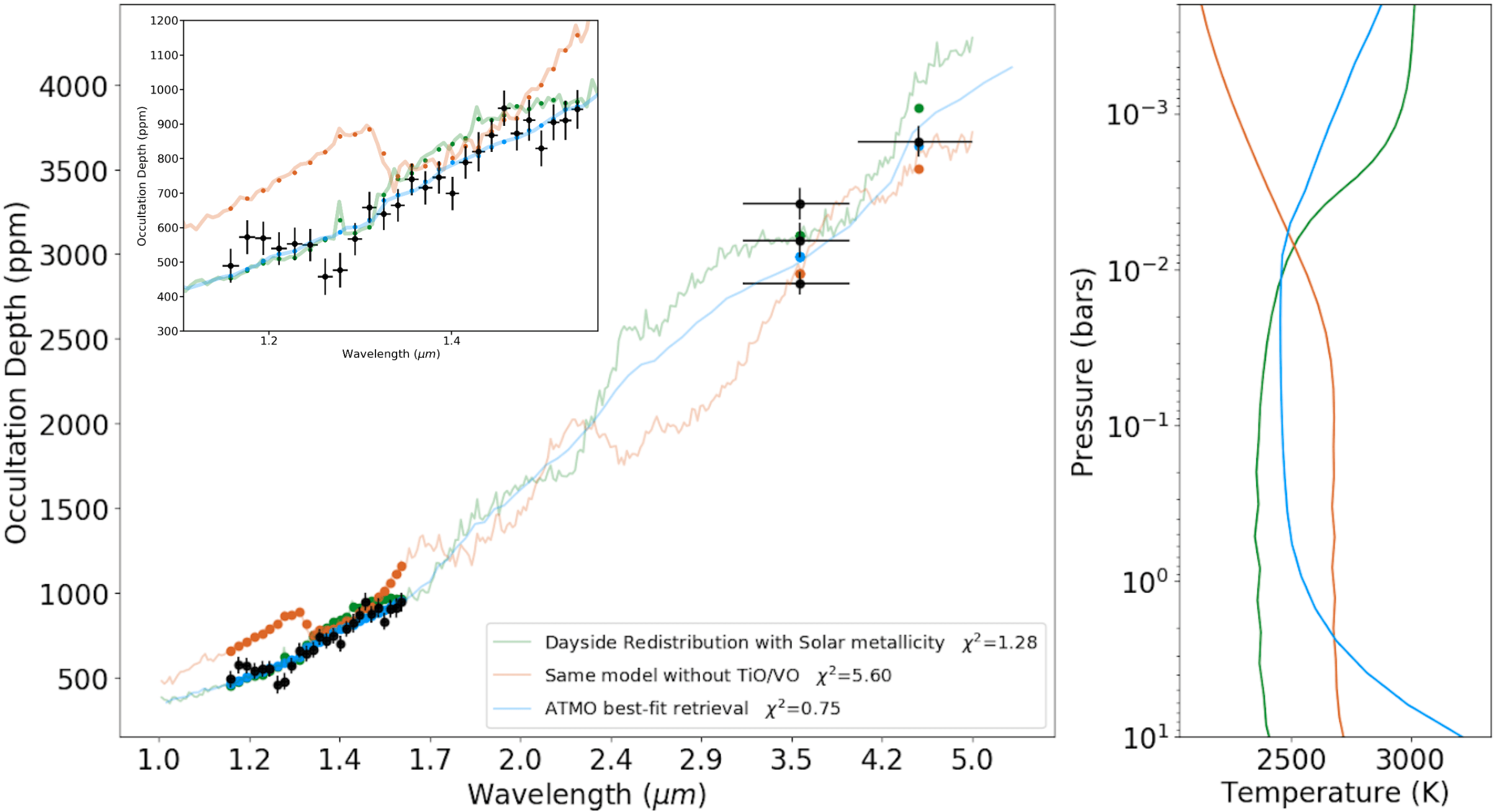
5.3 Emission spectrum
WASP-76b shows blackbody-like WFC3/G141 emission spectrum with muted water features but strong CO emission feature at Spitzer 4.5 band. The best-fit PHOENIX model shows dayside heat-redistribution and solar metallicity assuming equilibrium chemistry. We also ran a comparison PHOENIX model with the same setup but excluding TiO/VO to demonstrate the data strongly favors the presence of gaseous TiO/VO, as the is larger by 4.32, which is consistent with our finding in the transmission spectrum. In addition, we performed ATMO free-element equilibrium chemistry retrieval similarly to the transmission spectrum, though isotopic scattering was also included along with the thermal emission. The resulting ATMO best-fit model is highly consistent compared to the PHOENIX model with both models showing similar emission spectra and TP profiles (See Fig. 14). ATMO also favors solar metallicity in the retrieval posterior distribution (Fig. 18) but with less certainty at the C/O ratio since the muted water feature limits the constrains on the oxygen abundance. Both models favor a dayside temperature range of 2500 to 2600K around 1 bar and an inverted TP profile with temperature increasing to around 3000K at 0.1 mbars. Water starts to dissociate at such high temperature and low pressure region of the atmosphere as shown in Figure 15, therefore we do not see prominent water emission features. At deeper levels (1 bar) of the atmosphere, water vapor should still survive, but any absorption features will be obscured by the hotter continuum emission in the upper atmosphere layers. On the other hand, CO is able to survive in much higher altitude and temperature due to the strong triple bond structure. Indeed, we see clear CO emission features in the Spitzer 4.5 band.
5.4 Temperature inversion
We found clear temperature inversion (Figure 14) confirmed by ATMO and PHOENIX models. The Spitzer 4.5 CO emission feature strongly favors an inverted TP profile with higher temperature CO gas presence in the upper atmospheres. The transmission spectrum also favors an inverted TP profile as the retrievals need the higher temperature at the low pressures to boost the scale heights and the size of spectral features to better match the data. Theories have indicated inversion is caused by a combination of optical absorbers such as TiO (Hubeny et al., 2017; Fortney et al., 2008) and atomic metal absorption heating the upper layers with the lack of cooling from molecules like water (Lothringer et al., 2018; Gandhi & Madhusudhan, 2019). Our observed spectrum supports this paradigm with detection of TiO and atomic metal opacity in the transmission and muted water emission feature due to thermal dissociation at the highest altitudes. The detection of TiO and temperature inversion in the emission spectrum is also consistent with the independent analysis from Edwards et al. (2020) which reported similar findings.

5.5 Model comparison
ATMO best-fit model has the lower but PHOENIX generates a remarkable good fit in both transit and eclipse especially as only two parameters were varied in our grid of forward models. Retrieval frameworks find the best-fit spectrum through minimizing the likelihood which allows it to fine tune model parameters and better respond to smaller features in the data. Therefore, despite using an incomplete NUV opacity database, ATMO is able to produce better overall best-fit spectrum than the PHOENIX forward model. However, it is more important that ATMO and PHOENIX show good agreement on the general physical parameters including temperature structure, C/O ratio and chemical abundance. This gives us increased confidence in our conclusion, as both the retrieval and forward modeling methods agree.
6 Summary and Conclusions
We observed a combined total of 7 transits and 5 eclipses of the highly irradiated ultra-hot Jupiter WASP-76b using HST WFC3/STIS and . After correcting for the dilution effect of a nearby companion star, and refitting the orbital parameters, we performed retrieval analysis on the transmission and emission spectra using ATMO and a PHOENIX grid. The results from these independent modeling tools are in generally good agreement with the biggest difference being the completeness of NUV opacity lines of each model. We demonstrated the importance of including all atomic and molecular metal lines in the NUV to fully explain the excess transit depth observed between 0.3 and 0.4 in WASP-76b (Lothringer et al., 2020). Water vapor and TiO have also been directly detected in the transmission spectrum from STIS and WFC/G141 observations. Both transit and eclipse spectrum favor an inverted TP profile which is confirmed by both ATMO and PHOENIX models. The detection of TiO and ionized metals at the same time with an inverted TP profile are consistent with the theory of temperature inversion in ultra-hot Jupiters being caused by high altitude strong UV and optical absorbers heating up the upper layers. The lack of water emission due to dissociation at high temperature and altitude further drives the temperature inversion from the absence of cooling.
This study of WASP-76b supports some of our current understanding of ultra-hot Jupiter such as their thermal structure while poses new questions about their heavy metals composition that have previously been mostly ignored. It is evident more NUV atmosphere observations of ultra-hot Jupiters are needed for a more complete understanding of these unique planets. HST is currently the only observatory capable of observing in the NUV wavelength which will not be accessible with JWST. WASP-76b along with other ultra-hot Jupiters will be great targets for future detailed NUV studies with HST.
References
- Alexoudi et al. (2018) Alexoudi, X., Mallonn, M., von Essen, C., et al. 2018, A&A, 620, A142
- Allart et al. (2018) Allart, R., Bourrier, V., Lovis, C., et al. Science, 362, 1384
- Arcangeli et al. (2018) Arcangeli J., et al., 2018, ApJ, 855, L30
- Amundsen et al. (2014) Amundsen, D. S., Baraffe, I., Tremblin, P., et al. 2014, A&A, 564, A59
- Bohn et al. (2020) Bohn, A. J., Southworth, J., Ginski, C., et al. 2020, A&A
- Charbonneau et al. (2002) Charbonneau, D., Brown, T. M., Noyes, R. W., & Gilliland, R. L. 2002, ApJ, 568, 377
- Charbonneau et al. (2005) Charbonneau, D., Allen, L. E., Megeath, S. T., et al. 2005, ApJ, 626, 523.
- Choi et al. (2016) Choi, J., Dotter, A., Conroy, C., et al. 2016, ApJ, 823, 102
- Claret et al. (2013) Claret, A., Hauschildt, P. H., & Witte, S. 2013, A&A, 552, A16
- Cowan & Agol (2011) Cowan, N. B., & Agol, E. 2011, ApJ, 729, id.54.
- Crossfield et al. (2012) Crossfield, I. J. M., Barman, T., Hansen, B. M. S., Tanaka, I., & Kodama, T. 2012, ApJ, 760, 140
- Deming et al. (2005) Deming, D., Seager, S., Richardson, L. J., & Harrington, J. 2005, Nature, 434, 740.
- Deming et al. (2013) Deming, D., Wilkins, A., McCullough, P., et al. 2013, ApJ, 774, 95
- Deming et al. (2015) Deming, D., Knutson, H., Kammer, J., et al. 2015, ApJ, 805, 132
- Dotter et al. (2016) Dotter, A. 2016, ApJS, 222, 8
- Drummond et al. (2016) Drummond, B., Tremblin, P., Baraffe, I., et al. 2016, A&A, 594, A69
- Eastman (2017) J. Eastman, 2017ascl.soft10003E
- Eastman (2019) Eastman, J. D., Rodriguez, J. E., Agol, E., et al. 2019, arXiv e-prints, arXiv:1907.09480
- Eaton, Henry, & Fekel (2003) Eaton, J. A., Henry, G. W., & Fekel, F. C. 2003, in The Future of Small Telescopes in the New Millennium, Volume II - The Telescopes We Use, ed. T. D. Oswalt (Dordrecht: Kluwer), 189
- Edwards et al. (2020) Edwards, B., Changeat, Q., Baeyens, R., et al. 2020, AJ, 160, 8
- Ehrenreich et al. (2020) Ehrenreich, D., Lovis, C., Allart, R., et al. 2020, arXiv e-prints, arXiv:2003.05528
- Ehrenreich et al. (2015) Ehrenreich, D., Bourrier, V., Wheatley, P. J., et al. 2015, Nature, 522, 459
- Evans et al. (2017) Evans, T. M., et al. 2017, Nature, 548, 58.
- Evans et al. (2018) Evans, T. M., Sing, D. K., Goyal, J. M., et al. 2018, AJ, 156, 283
- Fu et al. (2017) Fu G., Deming D., Knutson H., Madhusudhan N., Mandell A., Fraine J., 2017, ApJ, 847, L22
- Foreman-Mackey et al. (2013) Foreman-Mackey, D., Hogg, D. W., Lang, D., & Goodman, J. 2013, PASP, 125, 306
- Fortney et al. (2008) Fortney, J. J., Lodders, K., Marley, M. S., & Freedman, R. S. 2008, ApJ, 678, 1419
- Fraine et al. (2014) Fraine, J., Deming, D., Benneke, B., et al. 2014, Nature, 513, 526
- Gandhi & Madhusudhan (2019) Gandhi, S. & Madhusudhan, N. 2019, MNRAS, 485, 5817
- Goyal et al. (2017) Goyal, J. M., Mayne, N., Sing, D. K., et al. 2017, arXiv:1710.10269
- Gaia Collaboration (2018b) Gaia Collaboration et al. 2018
- Garhart et al. (2020) Garhart, E., Deming, D., et al. eprint arXiv:1901.07040, in press for AJ.
- Haynes et al. (2015) Haynes, K., Mandell, A. M., Madhusudhan, N., Deming, D., Knutson, H. 2015, ApJ, 806, 146
- Heng et al. (2017) Heng, K., Kitzmann, D., 2017, MNRAS, 2017, stx1453. doi: 10.1093/mnras/stx1453
- Henry (1999) Henry, G. W. 1999, PASP, 111, 845
- Hubeny et al. (2017) Hubeny, I., Burrows, A., & Sudarsky, D. 2003, ApJ, 594, 1011
- Irwin et al. (2017) Irwin, J., Charbonneau, D., Nutzman, P., et al. 2008, ApJ, 681, 636
- Kirk et al. (2020) Kirk, J., Alam, M. K., Lopez-Morales, M., et al. 2020, arXiv e-prints, arXiv:2001.07667
- Kitzmann et al. (2018) Kitzmann, D., Heng, K., Rimmer, P. B., et al. 2018, ApJ, 863, 183
- Kreidberg et al. (2014a) Kreidberg, L., Bean, J. L., Désert, J.-M., et al. 2014, ApJL, 793, L27
- Kreidberg et al. (2014b) Kreidberg, L., Bean, J. L., Désert, J.-M., et al. 2014, Natur, 505, 69
- Kreidberg et al. (2015) Kreidberg, L., Line, M. R., Bean, J. L., et al. 2015, ApJ, 814, 66
- Kreidberg (2015) Kreidberg, L. 2015, PASP, 127, 1161
- Lothringer et al. (2018) Lothringer, J. D., Barman, T., & Koskinen, T. 2018, ApJ, 866, 27
- Lothringer & Barman (2019) Lothringer, J. D., & Barman, T. 2019, ApJ, 876, 69
- Lothringer et al. (2020) Lothringer, J. D., Fu, G., et al. 2020, ApJL, 898, 1
- Line et al. (2014) Line, M. R., Knutson, H., Wolf, A. S., & Yung, Y. L. 2014, ApJ, 783, 70
- Mandel & Agol (2002) Mandel K., Agol E., 2002, ApJ, 580, L171
- Madhusudhan et al. (2014) Madhusudhan, N., Crouzet, N., McCullough, P. R., Deming, D., & Hedges, C. 2014a, ApJL, 791, L9
- Mandell et al. (2013) Mandell, A. M., Haynes, K., Sinukoff, E., et al. 2013, ApJ, 779, 128
- Nikolov et al. (2013) Nikolov, N., Sing, D. K., Burrows, A. S., et al. 2015, MNRAS, 447, 463
- Nikolov et al. (2014) Nikolov N. et al., 2014, MNRAS, 437, 46
- Nikolov et al. (2015) Nikolov N. et al., 2015, MNRAS, 447, 463–478
- Nikolov et al. (2018) Nikolov, N., Sing, D. K., Fortney, J. J., et al. 2018, Nature, 557, 526
- Paxton et al. (2015) Paxton, B., Marchant, P., Schwab, J., et al. 2015, ApJS, 220, 15
- Pont et al. (2013) Pont, F., Sing, D. K., Gibson, N. P., et al. 2013, MNRAS, 432, 2917
- Parmentier et al. (2018) Parmentier, V., Line, M. R., Bean, J. L., et al. 2018, A&A, 617, A110
- Rodriguez et al. (2019) Rodriguez, J. E., Quinn, S. N., Huang, C. X., et al. 2019, AJ, 157, 191
- Seidel et al. (2019) Seidel, J. V., Ehrenreich, D., Wyttenbach, A., et al. 2019, A&A, 623, A166.
- Sing et al. (2011) Sing D. K. et al., 2011, MNRAS, 416, 1443
- Sing et al. (2016) Sing, D. K., Fortney, J. J., Nikolov, N., et al. 2016, Nature, 529, 59
- Sing et al. (2015) Sing, D. K. et al., 2015, MNRAS, 446, 2428
- Sing et al. (2015) Sing, D. K., Wakeford, H. R., Showman, A. P., et al. 2015, MNRAS, 446, 2428
- Sing et al. (2019) Sing, D. K., Lavvas, P., Ballester, G. E., et al. 2019, AJ, 158, 91
- Spake et al. (2018) J.J.Spake et al., Nature. 557, 68–70 (2018)
- Stevenson et al. (2014) Stevenson, K. B., Bean, J. L., Seifahrt, A., D´esert, J.-M., Madhusudhan, N., Bergmann, M., Kreidberg, L., & Homeier, D. 2014, AJ, 147, 161
- Stevenson et al. (2017) Stevenson, K. B., Line, M. R., Bean, J. L., et al. 2017, AJ, 153, 68
- Stevenson (2016) Stevenson, K. B. 2016, ApJL, 817, L16
- Stevenson et al. (2014) Stevenson, K. B., Desert, J.-M., Line, M. R., et al. 2014, Sci, 346, 838
- Tremblin et al. (2016) Tremblin, P., Amundsen, D. S., Chabrier, G., et al. 2016, ApJL, 817, L19
- Tremblin et al. (2015) Tremblin, P., Amundsen, D. S., Mourier, P., et al. 2015, ApJL, 804, L17
- Tsiaras et al. (2018) Tsiaras, A., Waldmann, I. P., Zingales, T., et al. 2017, AJ, 155, 4, 156, 15
- von Essen et al. (2020) von Essen, C., Mallonn, M., Hermansen, S., et al. 2020, submitted to A&A.
- Wollert & Brandner (2018) Wöllert, M. & Brandner, W. 2015, A&A, 579, A129
- West et al. (2016) West, R. G., et al., 2016, A&A, 585, A126
- Wakeford et al. (2013) Wakeford, H. R., Sing, D. K., Deming, D., et al. 2013, MNRAS, 435, 3481
- Wakeford et al. (2016) Wakeford, H. R., Sing, D. K., Evans, T., Deming, D., & Mandell, A. 2016, The Astrophysical Journal, 819, 10.
- Wakeford et al. (2017) Wakeford, H. R., Sing, D. S., Kataria, T., et al. 2017 Science, 356, 628
- Wilkins et al. (2014) Wilkins, A. N., Deming, D., Madhusudhan, N., Burrows, A., Knutson, H., McCullough, P., & Ranjan, S. 2014, ApJ, 783, 113.
- Zhang et al. (2018) Zhang, M. et al. 2018, arXiv:1811.11761
- Zhou et al. (2017) Zhou, Y., Apai, D. et al. Astron. J., 153, 243, 2017
| Parameter | Units | Values |
|---|---|---|
| Stellar Parameters: | ||
| Mass () | ||
| Radius () | ||
| Luminosity () | ||
| Density (cgs) | ||
| Surface gravity (cgs) | ||
| Effective Temperature (K) | ||
| Metallicity (dex) | ||
| Initial Metallicity | ||
| Age (Gyr) | ||
| Equal Evolutionary Phase | ||
| Companion Star Parameters: | ||
| Radius () | ||
| Effective Temperature (K) | ||
| Planetary Parameters: | ||
| Period (days) | ||
| Radius () | ||
| Mass () | ||
| Time of conjunction () | ||
| Optimal conjunction Time () | ||
| Semi-major axis (AU) | ||
| Inclination (Degrees) | ||
| Eccentricity | ||
| Argument of Periastron (Degrees) | ||
| Equilibrium temperature (K) | ||
| Tidal circularization timescale (Gyr) | ||
| RV semi-amplitude () | ||
| Log of RV semi-amplitude | ||
| Radius of planet in stellar radii | ||
| Semi-major axis in stellar radii | ||
| Transit depth (fraction) | ||
| Flux decrement at mid transit | ||
| Ingress/egress transit duration (days) | ||
| Total transit duration (days) | ||
| FWHM transit duration (days) | ||
| Transit Impact parameter | ||
| Eclipse impact parameter | ||
| Ingress/egress eclipse duration (days) | ||
| Total eclipse duration (days) | ||
| FWHM eclipse duration (days) | ||
| Blackbody eclipse depth at 3.6m (ppm) | ||
| Blackbody eclipse depth at 4.5m (ppm) | ||
| Density (cgs) | ||
| Surface gravity | ||
| Safronov Number | ||
| Incident Flux (109 erg s-1 cm-2) | ||
| Time of Periastron () | ||
| Time of eclipse () | ||
| Time of Ascending Node () | ||
| Time of Descending Node () | ||
| Minimum mass () | ||
| Mass ratio | ||
| Separation at mid transit | ||
| A priori non-grazing transit prob | ||
| A priori transit prob | ||
| A priori non-grazing eclipse prob | ||
| A priori eclipse prob | ||
| Wavelength midpoint (m) | Bin width (m) | Rp/Rs | Rp/Rs uncertainty | Dilution factor |
|---|---|---|---|---|
| 0.33000 | 0.04000 | 0.11329 | 0.00074 | 1.0086 |
| 0.38250 | 0.01250 | 0.11231 | 0.00058 | 1.00807 |
| 0.40315 | 0.00815 | 0.11110 | 0.00063 | 1.01406 |
| 0.41815 | 0.00685 | 0.11137 | 0.00061 | 1.01325 |
| 0.43250 | 0.00750 | 0.11021 | 0.00070 | 1.01498 |
| 0.44500 | 0.00500 | 0.11090 | 0.00062 | 1.01766 |
| 0.45500 | 0.00500 | 0.11104 | 0.00064 | 1.02015 |
| 0.46500 | 0.00500 | 0.11055 | 0.00060 | 1.02093 |
| 0.47500 | 0.00500 | 0.11114 | 0.00071 | 1.02133 |
| 0.48500 | 0.00500 | 0.11203 | 0.00069 | 1.0231 |
| 0.49500 | 0.00500 | 0.11126 | 0.00066 | 1.02192 |
| 0.50500 | 0.00500 | 0.11215 | 0.00074 | 1.02105 |
| 0.51500 | 0.00500 | 0.11202 | 0.00070 | 1.01997 |
| 0.52500 | 0.00500 | 0.11268 | 0.00067 | 1.02327 |
| 0.53500 | 0.00500 | 0.11235 | 0.00070 | 1.02497 |
| 0.54500 | 0.00500 | 0.11161 | 0.00068 | 1.02527 |
| 0.55500 | 0.00500 | 0.11187 | 0.00066 | 1.02664 |
| 0.56500 | 0.00500 | 0.11186 | 0.00069 | 1.02765 |
| 0.55500 | 0.00500 | 0.11107 | 0.00089 | 1.02664 |
| 0.56500 | 0.00500 | 0.11341 | 0.00099 | 1.02765 |
| 0.57500 | 0.00500 | 0.11250 | 0.00088 | 1.02814 |
| 0.58390 | 0.00390 | 0.11241 | 0.00108 | 1.02894 |
| 0.58955 | 0.00175 | 0.11278 | 0.00139 | 1.0275 |
| 0.59915 | 0.00785 | 0.11236 | 0.00082 | 1.02961 |
| 0.61350 | 0.00650 | 0.11223 | 0.00091 | 1.03001 |
| 0.62500 | 0.00500 | 0.11266 | 0.00080 | 1.03027 |
| 0.63750 | 0.00750 | 0.11275 | 0.00077 | 1.03116 |
| 0.65250 | 0.00750 | 0.11221 | 0.00076 | 1.03279 |
| 0.67000 | 0.01000 | 0.11187 | 0.00071 | 1.03279 |
| 0.69000 | 0.01000 | 0.11176 | 0.00074 | 1.03355 |
| 0.71000 | 0.01000 | 0.11286 | 0.00072 | 1.03411 |
| 0.73250 | 0.01250 | 0.11155 | 0.00070 | 1.03511 |
| 0.75475 | 0.00975 | 0.11194 | 0.00075 | 1.03628 |
| 0.76825 | 0.00375 | 0.11391 | 0.00197 | 1.03683 |
| 0.79100 | 0.01900 | 0.11158 | 0.00072 | 1.03747 |
| 0.82925 | 0.01925 | 0.11087 | 0.00079 | 1.03862 |
| 0.87350 | 0.02500 | 0.11249 | 0.00082 | 1.04058 |
| 0.96425 | 0.06575 | 0.11183 | 0.00094 | 1.04236 |
| 1.14250 | 0.00930 | 0.10965 | 0.00055 | 1.04738 |
| 1.16110 | 0.00930 | 0.10976 | 0.00055 | 1.04821 |
| 1.17970 | 0.00930 | 0.10865 | 0.00054 | 1.04882 |
| 1.19830 | 0.00930 | 0.11007 | 0.00054 | 1.04922 |
| 1.21690 | 0.00930 | 0.10930 | 0.00053 | 1.04999 |
| 1.23550 | 0.00930 | 0.10990 | 0.00054 | 1.05059 |
| 1.25410 | 0.00930 | 0.10993 | 0.00052 | 1.05126 |
| 1.27270 | 0.00930 | 0.10992 | 0.00052 | 1.05254 |
| 1.29130 | 0.00930 | 0.10884 | 0.00051 | 1.05325 |
| 1.30990 | 0.00930 | 0.10926 | 0.00051 | 1.05296 |
| 1.32850 | 0.00930 | 0.10943 | 0.00050 | 1.05367 |
| 1.34710 | 0.00930 | 0.11027 | 0.00050 | 1.05453 |
| 1.36570 | 0.00930 | 0.11071 | 0.00050 | 1.05525 |
| 1.38430 | 0.00930 | 0.11062 | 0.00050 | 1.056 |
| 1.40290 | 0.00930 | 0.10978 | 0.00049 | 1.05647 |
| 1.42150 | 0.00930 | 0.11047 | 0.00049 | 1.05618 |
| 1.44010 | 0.00930 | 0.11030 | 0.00048 | 1.05748 |
| 1.45870 | 0.00930 | 0.11113 | 0.00047 | 1.05799 |
| 1.47730 | 0.00930 | 0.11048 | 0.00046 | 1.05901 |
| 1.49590 | 0.00930 | 0.11029 | 0.00047 | 1.05928 |
| 1.51450 | 0.00930 | 0.11078 | 0.00047 | 1.06108 |
| 1.53310 | 0.00930 | 0.11064 | 0.00045 | 1.06235 |
| 1.55170 | 0.00930 | 0.11039 | 0.00045 | 1.06346 |
| 1.57030 | 0.00930 | 0.10974 | 0.00044 | 1.06339 |
| 1.58890 | 0.00930 | 0.11000 | 0.00043 | 1.06444 |
| 1.60750 | 0.00930 | 0.11008 | 0.00044 | 1.06581 |
| 3.55000 | 0.37500 | 0.11026 | 0.00048 | 1.06895 |
| 3.55000 | 0.37500 | 0.10862 | 0.00041 | 1.06895 |
| 4.49300 | 0.50750 | 0.11351 | 0.00056 | 1.06709 |
| Wavelength midpoint (m) | Bin width (m) | Occultation Depth (ppm) | Uncertainty (ppm) | Dilution factor |
|---|---|---|---|---|
| 1.1518 | 0.0093 | 490 | 49 | 1.04775 |
| 1.1704 | 0.0093 | 573 | 49 | 1.04869 |
| 1.1890 | 0.0093 | 570 | 48 | 1.04894 |
| 1.2076 | 0.0093 | 540 | 48 | 1.04953 |
| 1.2262 | 0.0093 | 553 | 47 | 1.05039 |
| 1.2448 | 0.0093 | 550 | 47 | 1.05078 |
| 1.2634 | 0.0093 | 458 | 53 | 1.05168 |
| 1.2820 | 0.0093 | 477 | 50 | 1.05360 |
| 1.3006 | 0.0093 | 567 | 47 | 1.05280 |
| 1.3192 | 0.0093 | 659 | 45 | 1.05328 |
| 1.3378 | 0.0093 | 640 | 47 | 1.05402 |
| 1.3564 | 0.0093 | 665 | 47 | 1.05485 |
| 1.3750 | 0.0093 | 740 | 46 | 1.05578 |
| 1.3936 | 0.0093 | 716 | 48 | 1.05623 |
| 1.4122 | 0.0093 | 746 | 47 | 1.05631 |
| 1.4308 | 0.0093 | 699 | 49 | 1.05671 |
| 1.4494 | 0.0093 | 789 | 47 | 1.05781 |
| 1.4680 | 0.0093 | 820 | 57 | 1.05830 |
| 1.4866 | 0.0093 | 868 | 48 | 1.05939 |
| 1.5052 | 0.0093 | 947 | 51 | 1.06001 |
| 1.5238 | 0.0093 | 874 | 50 | 1.06173 |
| 1.5424 | 0.0093 | 912 | 59 | 1.06301 |
| 1.5610 | 0.0093 | 830 | 52 | 1.06356 |
| 1.5796 | 0.0093 | 906 | 52 | 1.06397 |
| 1.5982 | 0.0093 | 911 | 57 | 1.06442 |
| 1.6168 | 0.0093 | 943 | 56 | 1.06572 |
| 3.5500 | 0.3750 | 2827 | 69 | 1.06895 |
| 3.5500 | 0.3750 | 3082 | 102 | 1.06895 |
| 3.5500 | 0.3750 | 3299 | 94 | 1.06895 |
| 4.4930 | 0.5075 | 3665 | 89 | 1.06709 |


