The hierarchy recurrences in local relaxation
Abstract
Inside a closed many-body system undergoing the unitary evolution, a small partition of the whole system exhibits a local relaxation. If the total degrees of freedom of the whole system is a large but finite number, such a local relaxation would come across a recurrence after a certain time, namely, the dynamics of the local system suddenly appear random after a well-ordered oscillatory decay process. It is found in this paper, for a collection of n two-level systems (TLSs), the local relaxation of one TLS within has a hierarchy structure hiding in the randomness after such a recurrence: similar recurrences appear in a periodical way, and the later recurrence brings in stronger randomness than the previous one. Both analytical and numerical results that we obtained well explains such hierarchy recurrences: the population of the local TLS (as an open system) diffuses out and regathers back periodically due the finite-size effect of the bath [the remaining TLSs]. We also find that the total correlation entropy, which sums up the entropy of all the n TLSs, approximately exhibit a monotonic increase; in contrast, the entropy of each single TLS increases and decreases from time to time, and the entropy of the whole n-body system keeps constant during the unitary evolution.
Introduction: When an open system is contacted with a bath infinitely large, the open system would approach a certain steady state after a long time relaxation. However, such an irreversible behavior cannot be seen in the dynamics of one or few-body systems. Thus the macroscopic irreversibility seems contradicted with the microscopic reversibility (Hobson, 1966; Prigogine, 1978; Mackey, 1989; Uffink, 2006; Swendsen, 2008).
One useful way to look through this problem is to study the system relaxation contacted with a finite bath, namely, the bath contains a finite number of degrees of freedom (DoF), and then consider its transition to the thermodynamics limit (Cramer et al., 2008; Flesch et al., 2008; Eisert et al., 2015; Xu et al., 2014). The open system and the bath as a whole isolate system always follows the unitary evolution and keeps a constant entropy as the initial state, while the open system itself seems relaxing towards a certain steady state, thus such a relaxation behavior of the open system itself is called the local relaxation (Cramer et al., 2008; Eisert et al., 2015; Flesch et al., 2008).
Due to the finite-size effect of the bath, the local relaxation of the open system would come across a recurrence after a certain time: at first the system dynamics shows a well-ordered oscillatory decay behavior, but then suddenly becomes random (Hänggi et al., 1990; Zwanzig, 2001; Cramer et al., 2008; Flesch et al., 2008; Eisert et al., 2015). With the increase of the DoF number in the bath, such a recurrence time appears much later, thus it does not show up in practice.
In this paper, we find that, in the region after such a recurrence, indeed there exists a hierarchy structure hiding in the randomness: similar recurrences appear in a periodical way, and the later recurrence brings in stronger randomness than the previous one, therefore, we call them hierarchy recurrences.
Here we study the dynamics of a chain of n two-level systems (TLSs). One of the TLSs is treated as the open system, and all the other TLSs make up a finite bath. We obtain a Bessel function expansion for the system dynamics, which well explains the appearance of such hierarchy recurrences. Further, we also find the physical reason for the appearance of such hierarchy recurrences: with the time increases, the population of the open system diffuses out and propagates in the finite bath (the periodic TLS chain); once the population regathers back to the open system, the system dynamics exhibits such a recurrence, and this process happens again and again, which gives rise to the hierarchy recurrences.
We also study the dynamics of the total correlation entropy of the n-body system, which sums up the entropy of all the n TLSs (Watanabe, 1960; Groisman et al., 2005; Zhou, 2008; Anza et al., 2020). It turns out the total correlation approximately exhibits a monotonic increasing behavior, and the increasing curve becomes more and more “smooth” with the increase of the bath size. Thus, the total correlation exhibits a quite similar behavior as the irreversible entropy increase in the standard thermodynamics (Lebowitz, 1993; Li, 2017; You and Li, 2018; Li, 2019). In contrast, the whole n-body system always keeps a constant due to the unitary evolution, and the entropy of each single TLS increases and decreases from time to time.
Local relaxation: We consider a chain of n TLSs. They have equal on-site energies (), and exchange energy with the nearest neighbors (interaction strengths ):
| (1) |
Here , , and , are the excited and ground states of the -th TLS.
Here site-0 is regarded as an open “system”, while all the other TLSs build up a finite “bath”. Initially, the “system” (site-0) starts from the excited state as its initial state, and all the TLSs in the “bath” start from the ground state. Thus effectively the “bath” has a temperature . And now we study the dynamics of the open “system”.
The Hamiltonian (1) is a quantum XX model (Sachdev, 2011), and the dynamics of the whole chain is exactly solvable. Applying the Jordan-Wigner transform, the Hamiltonian (1) becomes a fermionic one,
| (2) |
Under the periodic boundary condition, it can be further diagonalized by the Fourier transform , which reads , with the eigen mode energy .
The n-body chain as a whole isolated system follows the unitary evolution. From the above transformations, the above initial condition gives , and for the other , and that gives the following dynamics
| (3) |
where we call as the coherence function, and111Utilizing .
| (4a) | ||||
| (4b) | ||||
In the thermodynamics limit , becomes the Bessel function , which approaches zero when (Hänggi et al., 1990; Zwanzig, 2001; Cramer et al., 2008; Flesch et al., 2008; Eisert et al., 2015).
It can be seen from Eqs. (2, 3) that, each site always keeps a diagonal density state , where is the excited population of site-. Therefore, if the “bath” is infinitely large (), the “system” would reach and stay at the ground state after long time relaxation, namely, (here the limit is taken before ).
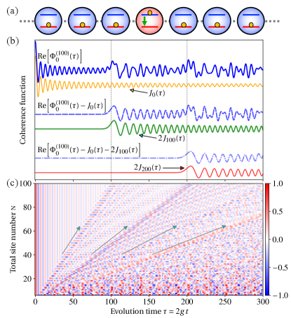
Scaling behavior of recurrences: If the “bath” is a finite one composed of TLSs, due to the finite-size effect, the above coherence functions exhibit a recurrence behavior222Precisely speaking, the recurrence behavior of the open system here is different from the Poincaré recurrence usually discussed in chaotic dynamics.: within the time , fits the above Bessel function (4b) quite closely and decays towards zero, but then it shows a “sudden bump” and starts to look random after [see the solid blue line in Fig. 1(b), is the recurrence time] (Hänggi et al., 1990; Zwanzig, 2001; Cramer et al., 2008; Flesch et al., 2008; Eisert et al., 2015).
Therefore, based on the local observation within a finite time smaller than , we may conclude the open “system” itself is relaxing towards a certain steady state, but indeed the full n-body state always keeps a pure state during the unitary evolution. With the increase of the size n, the recurrence time becomes larger and larger, thus such a recurrence behavior does not show up in practice.
In Fig. 1(c), the scaling behavior of for different sizes n is shown. Besides the above recurrence appearing around , it is worth noting that some well-organized recurrence patterns also appear in the region . It can be seen similar recurrences also appear periodically around for [see the arrows in Fig. 1(c)]. Moreover, each recurrence seems bringing in stronger randomness to than the previous one, which forms a hierarchy structure, thus we call them hierarchy recurrences.
We find that the appearance of such hierarchy recurrences can be explained by the following expansion of [Eq. (4a)], that is,
| (5) |
Here we used the relation , with as an arbitrary integer.
For example, site-0 () gives a simple Bessel function series [using ]333When , the function series converges pointwise to but not uniformly.
| (6) |
For a large n, the Bessel function in the area , and starts to exhibit significant oscillations after [see in Fig. 1(b)]. Therefore, in the above expansion of , each term contributes a “sudden bump” around , and this is just why the above recurrences appear around ().
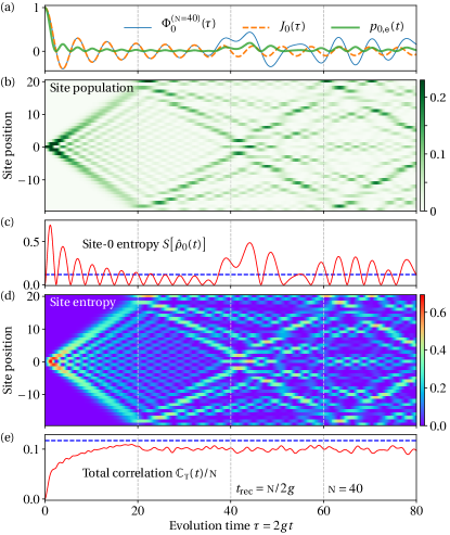
Population propagation: The population dynamics of all the n TLSs is shown in Fig. 2(b), i.e., , and a propagation pattern is clearly seen. Initially, the population distribution of the n TLSs forms a “cusp” around site-0 [, and for ]. Within the time , the initial population “cusp” on site-0 propagates towards the two directions of the periodic chain, and the propagation “speed” is almost a constant (Lieb and Robinson, 1972; Ganahl et al., 2012). This constant speed also can be seen from the leading terms of [for , see Eq. (5)]: the leading Bessel function indicates the first “sudden bump” of site- appears around , which linearly depends on the distance to site-0 [here site- and site- are the same one due to the periodic boundary condition].
The two-side propagations would meet each other at the periodic boundaries at , and then regathers back to site-0 again. Notice that this is just the moment that exhibits its first recurrence (, see the dashed vertical lines in Fig. 2). The propagation regathered back would be superposed with the original one, and that makes the system dynamics appear more random. Clearly, since such propagation and regathering happens again and again, the “system” (site-0) experiences the above hierarchy recurrences periodically around .
Total correlation entropy: Now we consider the entropy dynamics in this system. The n-body chain as a whole isolated system follows the unitary evolution, thus its von Neumann entropy always keeps zero as the initial state. Since initially the “bath” has a zero temperature , the thermal entropy in the standard thermodynamics cannot be used here either (Santos et al., 2017).
Notice that, in practical observations, indeed the full n-body state is usually not directly accessible for local measurements, and it is the few-body observables that can be directly measured (Swendsen, 2008; Li, 2019; Strasberg, 2019). Therefore, here we consider the dynamics of the total correlation entropy of the n-body state , that is (Watanabe, 1960; Groisman et al., 2005; Zhou, 2008; Anza et al., 2020),
| (7) |
where are the reduced 1-body states. For bipartite systems (), it just returns the mutual information (Nielsen and Chuang, 2000; Li, 2017, 2019; You and Li, 2018).
It turns out, the entropy of each single TLS is increasing and decreasing from time to time, and they also have the above recurrence behavior [Fig. 3(c, d)]. In contrast, their summation as the total correlation approximately exhibits a monotonic increasing behavior [except still carrying small fluctuations, see Fig. 2(e)]. Moreover, with the increase of the chain size n, the increasing curve of appears more and more “smooth” [Fig. 3(a-c)]. Clearly, this is quite similar with the behavior of the irreversible entropy production during the relaxation process in the standard thermodynamics (Spohn, 1978; de Groot and Mazur, 1962; Kondepudi and Prigogine, 2014; Nicolis and Prigogine, 1977).
Now we consider the correlation maximum that might achieve (Jaynes, 1957). With the help of Lagrangian multipliers, under the constraints (1) (probability normalization) and (2) (excitation number conservation), the maximum of is obtained as
| (8) |
The maximum is achieved when all the n TLSs have the same populations .
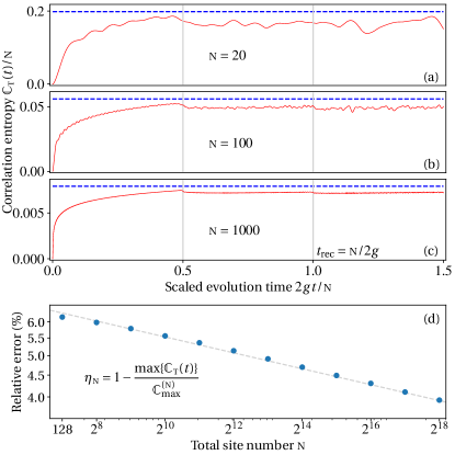
Under the scaled time , the correlation evolutions for different sizes n appear quite similar to each other [Fig. 3(a-c)]. They all approach their upper bound closely, and come across a “sudden bump” around half of the recurrence time (indeed this is just the moment the two-side propagations meet each other at ).
We denote as the relative error between and the correlation maximum . With the increase of the size n, the error decays slowly towards zero [approximately with , see Fig. 3(d)]. In the thermodynamic limit , we may expect could reach the maximum .
In this sense, the above correlation maximization effectively gives a pseudo-equilibrium state , where , and the whole n-body state “looks” like approaching this pseudo-equilibrium state during the unitary evolution (Cramer et al., 2008). But we emphasize indeed and never have any steady states when , and always keeps a pure state.
The increasing rate of the above total correlation (7) also can be rewritten in the form of relative entropy (Spohn, 1978; Esposito et al., 2010; Manzano et al., 2016; Ptaszyński and Esposito, 2019)
| (9) |
where is the relative entropy. Approximately, the reference state here can be replaced by the pseudo-equilibrium state .
We emphasize that the pseudo-equilibrium state here is determined by the above correlation maximization, but irrelevant with the on-site energy and the interaction strength , thus it is different from the canonical state like . If the on-site energy , all the above results for the system dynamics still remains the same.
Moreover, when , the status of and are indeed reversed: initially, the open “system” starts from the ground state while the TLSs in the “bath” start from the excited state. Therefore, effectively the “bath” has a negative temperature (Landau and Lifshitz, 1980; Ramsey, 1956). Notice that all the above results of the total correlation entropy still applies in this situation.
Summary: In this paper, we study the local relaxation process of an open system contacted with a finite bath. We find that, due to the finite-size effect of the bath, the local relaxation of the open system exhibits hierarchy recurrences periodically, which makes the system dynamics appear more and more random. Essentially, that is because the energy diffuses out of the open system regathers back from the finite bath again and again. During the unitary evolution, the open system and the bath as a whole isolate system keeps a constant entropy, and the entropy of each single TLS increases and decreases from time to time, while the total correlation entropy approximately exhibits a monotonic increasing behavior, which is similar as the irreversible entropy increase in the standard thermodynamics (Lebowitz, 1993; Li, 2017; You and Li, 2018; Li, 2019). We emphasize throughout the above discussions there is no average on time or any random configurations. The quantum XX model here could be realized in many physical systems, such as optical lattices (Trotzky et al., 2012), superconducting circuits (Ye et al., 2019; Orell et al., 2019), and ion trap arrays (Smith et al., 2016; Xiong et al., 2018).
Acknowledgment – S.-W. Li appreciates for the helpful discussions with J. Chen, B. Garraway, N. Wu, D. Z. Xu, Y.-N. You. This study is supported by NSF of China (Grant No. 11905007), Beijing Institute of Technology Research Fund Program for Young Scholars.
References
- Hobson (1966) A. Hobson, Am. J. Phys. 34, 411 (1966).
- Prigogine (1978) I. Prigogine, Science 201, 777 (1978).
- Mackey (1989) M. C. Mackey, Rev. Mod. Phys. 61, 981 (1989).
- Uffink (2006) J. Uffink, in Philosophy of Physics, Handbook of the Philosophy of Science (North Holland, Amsterdam, 2006) p. 923.
- Swendsen (2008) R. H. Swendsen, Am. J. Phys. 76, 643 (2008).
- Cramer et al. (2008) M. Cramer, C. M. Dawson, J. Eisert, and T. J. Osborne, Phys. Rev. Lett. 100, 030602 (2008).
- Flesch et al. (2008) A. Flesch, M. Cramer, I. P. McCulloch, U. Schollwöck, and J. Eisert, Phys. Rev. A 78, 033608 (2008).
- Eisert et al. (2015) J. Eisert, M. Friesdorf, and C. Gogolin, Nature Phys. 11, 124 (2015).
- Xu et al. (2014) D. Z. Xu, S.-W. Li, X. F. Liu, and C. P. Sun, Phys. Rev. E 90, 062125 (2014).
- Hänggi et al. (1990) P. Hänggi, P. Talkner, and M. Borkovec, Rev. Mod. Phys. 62, 251 (1990).
- Zwanzig (2001) R. Zwanzig, Nonequilibrium statistical mechanics, 1st ed. (Oxford University Press, Oxford, 2001).
- Watanabe (1960) S. Watanabe, IBM J. Res. Dev. 4, 66 (1960).
- Groisman et al. (2005) B. Groisman, S. Popescu, and A. Winter, Phys. Rev. A 72, 032317 (2005).
- Zhou (2008) D. L. Zhou, Phys. Rev. Lett. 101, 180505 (2008).
- Anza et al. (2020) F. Anza, F. Pietracaprina, and J. Goold, Quantum 4, 250 (2020).
- Lebowitz (1993) J. L. Lebowitz, Physica A 194, 1 (1993).
- Li (2017) S.-W. Li, Phys. Rev. E 96, 012139 (2017).
- You and Li (2018) Y.-N. You and S.-W. Li, Phys. Rev. A 97, 012114 (2018).
- Li (2019) S.-W. Li, Entropy 21, 111 (2019).
- Sachdev (2011) S. Sachdev, Quantum phase transitions, 2nd ed. (Cambridge University Press, Cambridge ; New York, 2011).
- Lieb and Robinson (1972) E. H. Lieb and D. W. Robinson, Commun. Math. Phys. 28, 251 (1972).
- Ganahl et al. (2012) M. Ganahl, E. Rabel, F. H. L. Essler, and H. G. Evertz, Phys. Rev. Lett. 108, 077206 (2012).
- Santos et al. (2017) J. P. Santos, G. T. Landi, and M. Paternostro, Phys. Rev. Lett. 118, 220601 (2017).
- Strasberg (2019) P. Strasberg, arXiv:1906.09933 (2019).
- Nielsen and Chuang (2000) M. A. Nielsen and I. L. Chuang, Quantum Computation and Quantum Information (Cambridge University Press, Cambridge, England, 2000).
- Spohn (1978) H. Spohn, J. Math. Phys. 19, 1227 (1978).
- de Groot and Mazur (1962) S. R. de Groot and P. Mazur, Non-equilibrium thermodynamics (North-Holland, Amsterdam, 1962).
- Kondepudi and Prigogine (2014) D. Kondepudi and I. Prigogine, Modern Thermodynamics (John Wiley & Sons, Ltd, Chichester, UK, 2014).
- Nicolis and Prigogine (1977) G. Nicolis and I. Prigogine, Self-Organization in Nonequilibrium Systems, 1st ed. (Wiley, New York, 1977).
- Jaynes (1957) E. T. Jaynes, Phys. Rev. 106, 620 (1957).
- Esposito et al. (2010) M. Esposito, K. Lindenberg, and C. Van den Broeck, New J. Phys. 12, 013013 (2010).
- Manzano et al. (2016) G. Manzano, F. Galve, R. Zambrini, and J. M. R. Parrondo, Phys. Rev. E 93, 052120 (2016).
- Ptaszyński and Esposito (2019) K. Ptaszyński and M. Esposito, Phys. Rev. Lett. 123, 200603 (2019).
- Landau and Lifshitz (1980) L. Landau and E. Lifshitz, Statistical Physics, Part 1 (Butterworth-Heinemann, Oxford, 1980).
- Ramsey (1956) N. F. Ramsey, Phys. Rev. 103, 20 (1956).
- Trotzky et al. (2012) S. Trotzky, Y.-A. Chen, A. Flesch, I. P. McCulloch, U. Schollwöck, J. Eisert, and I. Bloch, Nature Physics 8, 325 (2012).
- Ye et al. (2019) Y. Ye, Z.-Y. Ge, Y. Wu, S. Wang, M. Gong, Y.-R. Zhang, Q. Zhu, R. Yang, S. Li, F. Liang, J. Lin, Y. Xu, C. Guo, L. Sun, C. Cheng, N. Ma, Z. Y. Meng, H. Deng, H. Rong, C.-Y. Lu, C.-Z. Peng, H. Fan, X. Zhu, and J.-W. Pan, Phys. Rev. Lett. 123, 050502 (2019).
- Orell et al. (2019) T. Orell, A. A. Michailidis, M. Serbyn, and M. Silveri, Phys. Rev. B 100, 134504 (2019).
- Smith et al. (2016) J. Smith, A. Lee, P. Richerme, B. Neyenhuis, P. W. Hess, P. Hauke, M. Heyl, D. A. Huse, and C. Monroe, Nature Physics 12, 907 (2016).
- Xiong et al. (2018) T. P. Xiong, L. L. Yan, F. Zhou, K. Rehan, D. F. Liang, L. Chen, W. L. Yang, Z. H. Ma, M. Feng, and V. Vedral, Phys. Rev. Lett. 120, 010601 (2018).