Department of Computer Science, Princeton University, United [email protected]://orcid.org/0000-0001-8542-0247Department of Computer Science, Princeton University, United [email protected]://orcid.org/0000-0002-6398-3097 Department of Computer Science, ETH Zurich, [email protected]://orcid.org/0009-0002-7028-2595 \CopyrightBernard Chazelle, Kritkorn Karntikoon, and Jakob Nogler {CCSXML} <ccs2012> <concept> <concept_id>10003752.10010061</concept_id> <concept_desc>Theory of computation Randomness, geometry and discrete structures</concept_desc> <concept_significance>500</concept_significance> </concept> </ccs2012> \ccsdesc[500]Theory of computation Randomness, geometry and discrete structures \fundingThis work was supported in part by NSF grant CCF-2006125. \EventEditorsJohn Q. Open and Joan R. Access \EventNoEds2 \EventLongTitle42nd Conference on Very Important Topics (CVIT 2016) \EventShortTitleCVIT 2016 \EventAcronymCVIT \EventYear2016 \EventDateDecember 24–27, 2016 \EventLocationLittle Whinging, United Kingdom \EventLogo \SeriesVolume42 \ArticleNo23
The Geometry of Cyclical Social Trends
Abstract
We investigate the emergence of periodic behavior in opinion dynamics and its underlying geometry. For this, we use a bounded-confidence model with contrarian agents in a convolution social network. This means that agents adapt their opinions by interacting with their neighbors in a time-varying social network. Being contrarian, the agents are kept from reaching consensus. This is the key feature that allows the emergence of cyclical trends. We show that the systems either converge to nonconsensual equilibrium or are attracted to periodic or quasi-periodic orbits. We bound the dimension of the attractors and the period of cyclical trends. We exhibit instances where each orbit is dense and uniformly distributed within its attractor. We also investigate the case of randomly changing social networks.
keywords:
opinion dynamics, Minkowski sums, equidistribution, periodicity1 Introduction
Much of the work in the area of opinion dynamics has focused on consensus and polarization [3, 14]. Typical questions include: How do agents come to agree or disagree? How do exogenous forces drive them to consensus? How long does it take for opinion formation to settle? Largely left out of the discussion has been the emergence of cyclical trends. Periodic patterns in opinions and preferences is a complex, multifactorial social phenomenon beyond the scope of this work [24]. A question worth examining, however, is whether the process conceals deeper mathematical structure. The purpose of this work is to show that it is, indeed, the case.
This work began with a thought experiment and a computer simulation. The latter revealed highly unexpected behavior, which in turn compelled us to search for an explanation. Our main result is a proof that adding a simple contrarian rule to the classic bounded-confidence model suffices to produce quasi-periodic trajectories. The model is a slight variant of the classic HK framework: a finite collection of agents hold opinions on several topics, which they update at discrete time steps by consulting their neighbors in a (time-varying) social network. The modification is the addition of a simple repulsive force field that keep agents away from tight consensus. The idea is partly inspired by swarming dynamics. For example, birds refrain from flocking too closely. Likewise, near-consensus on a large enough scale tends to induce contrarian reactions among agents [1, 20]. Some political scientists have pointed to contrarianism as one of the reasons for the closeness of some national elections [19, 18].
One of the paradoxical observations we sought to elucidate was why cyclic trends in social networks seem oblivious to the initial opinions of one’s friends: specifically, it is not specific distributions of initial opinions that produce oscillations but, rather, the recurrence of certain symmetries in the networks. We prove that the condition is sufficient (though its necessity is still open). Another mystery was why contrarian opinions tend to orbit toward an attractor whose dimensionality is independent of the number of opinions held by a single agent. These attracting sets are typically Minkowski sums of ellipses. They emerge algorithmically and constitute a natural focus of interest in distributed computational geometry.
Our inquiry builds on the pioneering work of French [16], DeGroot [10], Friedkin & Johnsen [17], and Deffuant et al. [9]. The model we use is a minor modification of the bounded-confidence model model [5, 21]. A Hegselmann-Krause (HK) system consists of agents, each one represented by a point in . The coordinates for each agent represent their current opinions on different topics: thus, is the dimension of the opinion space. At any (discrete) time, each agent moves to the mass center of the agents within a fixed distance , which represents its radius of influence (Fig. 1). This step is repeated ad infinitum. Formally, the agents are positioned at at time and for any ,
| (1) |

Interpreting each as the set of neighbors of agent defines the social network at time . In the special case where all the radii of influence are equal , convergence into fixed-point clusters occurs within a polynomial number of steps [4, 13, 25]. Computer simulation suggests that the same remains true even when the radii differ but a proof has remained elusive. For cyclical trends to emerge, the social networks require a higher degree of underlying structure. In this work, we assume vertex transitivity (via Cayley graphs), which stipulates that agents cannot be distinguished by their local environment. Before defining the model formally in the next section, we summarize our main findings.
-
•
Undirected networks always drive the agents to nonconsensual convergence, ie, to fixed points at which they “agree to disagree.” For their behavior to become periodic or quasi-periodic, the social networks need to be directed. We prove that such systems either converge or are attracted to periodic or quasi-periodic orbits. We give precise formulas for the orbits.
-
•
We investigate the geometry of the attractors (Fig. 2). We bound the rotation number, which indicates the speed at which (quasi)-periodic opinions undergo a full cycle. We exhibit instances where each limiting orbit forms a set that is dense and, in fact, uniformly distributed on its attractor.
-
•
We explore the case of social networks changing randomly at each step. We prove the surprising result that the dimension of the attractor can decrease because of the randomization. This is a rare case where adding entropy to a system can reduce its dimensionality.
The dynamics of contrarian views has been studied before [1, 11, 15, 19, 18, 20, 26] but, to our knowledge, not for the purpose of explaining cyclical trends. Our mathematical findings can be viewed as a grand generalization of the affine-invariant evolution of planar polygons studied in [6, 8, 12, 22].

2 Contrarian Opinion Dynamics
The social network is a time-dependent Cayley graph over an abelian group. All finite abelian groups are isomorphic to a direct sum of cyclic groups . For notational convenience, we set . We regard the toral grid as a vector space, and we write . Let be the position of agent in at time . We fix and abbreviate it as . Choose such that and let be an infinite sequence of subsets of . For technical convenience, we assume that each set spans the vector space ; hence . In the spirit of HK systems, we define the dynamics as follows: for
| (2) |
Because of the presence of the “self-confidence” weight , we may assume that the convolution set does not contain the origin . If we view each as a row vector in , the update (2) specifies an -by- stochastic matrix . Let denote the -by- matrix whose rows are the agent positions , for . We have . The matrix may not be symmetric but it is always doubly-stochastic. This means that the mass center is time-invariant. Since the dynamics itself is translation-invariant, we are free to move the mass center to the origin, which we do by assuming , where denotes .
Obviously, some initial conditions are uninteresting: for example, . For this reason, we choose randomly; specifically, each is picked iid from the dimensional normal distribution . In the following, we use the phrase “with high probability,” to refer to an event occurring with probability at least , for any fixed . Once we’ve picked the matrix randomly, we place the mass center of the agents at the origin by subtracting its displacement from the origin: .
The agents will be attracted to the origin to form a single-point cluster of consensus in the limit. Responding to their contrarian nature, the agents will restore mutual differences by boosting the own opinions. For that reason we consider the scaled dynamics: and, for ,
| (3) |
where is chosen so that the diameter of the system remains roughly constant. Since scaling leaves the salient topological and geometric properties of the dynamics unchanged, the precise definition of can vary to fit analytical (or even visual) needs.
2.1 Preliminaries
We define the directed graph at time , where and . For clarity, we drop the subscript for the remainder of this section; so we write for .
Lemma 2.1.
The convolution set spans the vector space if and only if the graph is strongly connected.
Proof 2.2.
If spans , then for any pair , there exist , for each , such that . The right-hand side specifies edges (sum taken over ) that form a path from to ; therefore is strongly connected. Conversely, assuming the latter, there is a path from to : , with and . Thus, , where ; therefore spans .
Our assumption about implies that each is strongly connected. The presence of the weight in (2) ensures that the diagonal of is positive. Together with the strong connnectivity assumption, this makes the matrix primitive, meaning that , for some . By the Perron-Frobenius theorem [27], all the eigenvalues of lie strictly inside the unit circle in , except for the dominant eigenvalue 1, which has multiplicity . For any , we write , where . We define the vector and easily verify that forms an orthogonal eigenbasis for . The eigenvalue corresponding to satisfies
We conclude:
Lemma 2.3.
Each corresponds to a distinct eigenvector , which together form an orthogonal basis for . The corresponding eigenvalue is given by
We define and denote by the set of subdominant eigenvectors. The argument of plays a key role in our discussion, so we define such that , with . By (6), for , so is well defined.
2.2 The evolution of opinions
We begin with the case of a fixed convolution set . The initial position of the agents is expressed in eigenspace as . Let denote the row vector . Because , for ,
| (4) |
Lemma 2.4.
With high probability, for all ,
Proof 2.5.
Let be the first column of the matrix . For each , by the initialization of the system, , where and . Given , is orthogonal to ; hence . Since the random vector is unbiased and , it follows that . Thus, the first coordinate of is of the form , where and are sampled (not independently) from and , respectively, such that . Thus, with probability at most . Conversely, by the inequality erfc for , we find that , with probability at least , for any ; hence , with probability at least . Setting and using a union bound completes the proof.
We upscale the system by setting ; hence .
Theorem 2.6.
Let and be the row vectors whose -th coordinates () are and , respectively. With high probability, for each , the agent is attracted to the trajectory of , where
| (5) |
Let be the third largest (upscaled) eigenvalue, measured in distinct moduli. The error of the approximation decays exponentially fast as a function of :
Proof 2.7.
Since the eigenvalues sum up to tr and 1 has multiplicity 1, we have ; hence, by ,
| (6) |
Writing and , we have for ; recall that . By (4), it follows that
| (7) |
where, by Lemma 2.4, with high probability,
The lower bound of the lemma implies that, for any ,
For large enough , the sum in (7) dominates with high probability, while the latter decays exponentially fast. Thus the dynamics is asymptotically equivalent to . Recall that ; since, for , has modulus 1, it is equal to . This implies that . Because is real, we can ignore the imaginary part when expanding the expression above, which completes the proof.
2.3 Geometric investigations
The trajectory is called the limiting orbit.111The phase space of the dynamical system is , but by abuse of notation we use the word “orbit” to refer the trajectory of a single agent, which lies in . Theorem 2.6 indicates that, with high probability, every orbit is attracted to its limiting form at an exponential rate, so we may focus on the latter. Given the initial placement of the agents, all the limiting orbits lie in the set , expressed in parametric form by
| (8) |
Recall that and are row vectors in . The attractor is the Minkowski sum of a number of ellipses. We examine the geometric structure and explain how the limiting orbits embed into it. To do that, we break up the sum (5) into three parts. Given , we know that by (6), so there remain the following cases for the subdominant eigenvalues:
-
•
real : the contribution to the sum is , where is the row vector
(9) -
•
real : the contribution is , where, likewise, is the row vector
(10) -
•
nonreal : we can assume that since the conjugate eigenvalue is also present in . The contribution of an eigenvalue is the same as that of its conjugate since and . So the contribution of a given is equal to , where
which we can expand as , where222 .
(11)
Putting all three contributions together, we find
| (12) |
where is the set of distinct for and all other quantities are defined in (9, 10, 11). See Figure 3 for an illustration of a doubly-elliptical orbit around its torus-like attractor.

2.3.1 Generic elliptical attraction
We prove that, for almost all values of the self-confidence weight , the set generates either a single real eigenvalue or two complex conjugate ones. By (12), this shows that almost every limiting orbit is either a single fixed point or a subset of an ellipse in .
Theorem 2.8.
There exists a set of at most reals such that the set is associated with either a single real eigenvalue or two complex conjugate ones, for any .
The system is called regular if . For such a system, either (i) and , or (ii) and exactly one of or equals . In other words, by (12), we have three cases depending on the subdominant eigenvalues:
| (13) |
Lemma 2.9.
Consider a triangle and let and . Let be the origin and assume that the segments and are of the same length (Fig. 4); then the identity holds.
Proof 2.10.
Let be the midpoint of . The segment lies on the perpendicular bisector of , so it is orthogonal to ; hence to . Thus, . Since , the lemma follows from .
Proof 2.11 (Proof of Theorem 2.8).
Pick two distinct . Applying Lemma 2.9 in the complex plane, we set: ; ; and ; thus and , which implies that the segments and are of the same length. Abusing notation by treating as both vectors and complex numbers, we have ; therefore,
-
1.
If , then , which in turn implies that ; hence and .
-
2.
If , then is unique: .
We form by including all of the numbers , with .
In some cases, regularity holds with no need to exclude values of :
Theorem 2.12.
If forms a basis of and is prime, then and produces exactly two eigenvalues: and its conjugate.
Proof 2.13.
By Lemma 2.3, . Fix nonzero . Because is prime and the vectors from form a basis over the field , the -by- matrix whose -th row is is nonsingular. This implies that, in the sum , the exponent sequence appears for exactly one value and the same is true of . This holds true of any one-hot vector with a single at any place and elsewhere. This means that, for values of , the eigenvalue is of the form or its conjugate. Simple examination shows that these are precisely the subdominant eigenvalues.
2.3.2 The case of cycle convolutions
It is useful to consider the case of a single cycle: . For convenience, we momentarily assume that is prime and that ; both assumptions will be dropped in subsequent sections.
Lemma 2.14.
Each eigenvalue is simple.
Proof 2.15.
Because is prime, the cyclotomic polynomial for is . It is the minimal polynomial for , which is unique. Note that , since . Given , we define the polynomial in the quotient ring of rational polynomials . Sorting the summands by degree modulo , we have , for nonnegative integers , where . If , for some , then, by Lemma 2.3, ; hence divides . Because the latter is of degree at most , it is either identically zero or equal to up to a rational factor . In the second case,
This implies that , for all , which contradicts the fact that ; therefore, .
-
1.
If , then ; hence and , ie, .
-
2.
If , then let . Because is a field, the roots of unity in are distinct; hence . It follows that and ; therefore, for some permutation of order , we have , for all . Summing up both sides over gives us ; hence , since .
By (13), the limiting orbit is of the form or if the subdominant eigenvalue is real. Otherwise, the orbit of an agent approaches a single ellipse in : for some , .
2.3.3 Opinion velocities
Assume that the system is regular, so is associated with either a single real eigenvalue or two complex conjugate ones. If , by (12), every agent converges to a fixed point of the attractor or its limiting orbit has a period of 2. The other case is more interesting. The agent approaches its limiting orbit, which is periodic or quasi-periodic. The rotation number, , is the (average) fraction of a whole rotation covered in a single step. It measures the speed at which the agent cycles around its orbit. We prove a lower bound on that speed.333Its upper bound is .
Theorem 2.16.
The rotation number of a regular system satisfies .
Proof 2.17.
Of course, this assumes that . Fix and let ; further, assume that is nonzero, hence imaginary. We have , where is a vector in . It follows that , for an -by- matrix whose nonzero elements are and whose rows are given by . Thus, is an imaginary eigenvalue of ; hence a complex root of the characteristic polynomial . Let be the rank of and let be its nonzero eigenvalues. Expansion of the determinant gives us a sum of monomials of the form , for , where . The subset of them given by add up to the product of the nonzero eigenvalues (times ); hence . Label the nonzero eigenvalue of smallest modulus. The sum of the squared moduli of the eigenvalues of a matrix is at most the square of its Frobenius norm; hence no eigenvalue of can have a modulus larger than and, therefore
| (14) |
Since , it follows from (6) that . Thus,
With assumed to be nonreal, Lemma 2.3 implies that so is ; hence . Applying (14) completes the proof.
Our next result formalizes the intuitive fact that self-confidence slows down motion. Self-assured agents are reluctant to change opinions.
Theorem 2.18.
The rotation number of a regular system cannot increase with .
Proof 2.19.
We must have . Let be (an) eigenvalue corresponding to the unique angle in ; recall that . As we replace by , we use the prime sign with all relevant quantities post-substitution. Thus, the subdominant eigenvalue for associated with is denoted by ; again, we assume that . Note that might not necessarily be equal to ; hence the case analysis:
-
•
: Using the same notation for complex numbers and the points in the plane they represent (Fig. 5), we see that lies in (the relative interior of) the segment ; hence .
-
•
: We prove that, as illustrated in Fig. 5, all three conditions , , and , cannot hold at the same time, which will establish the theorem. If we increase continuously from to , decreases continuously. (We use the argument to denote the fact that corresponds to the eigenvalue defined with replaced by .) Since, at the end of that motion, , by continuity we have , where . To simplify the notation, we repurpose the use of the prime superscript to refer to (eg, ). So, we now have and . It follows that (i) the point lies in the pie slice of radius running counterclockwise from to on the real axis. Also, because and , setting as before in Lemma 2.9 shows that (ii) .444The keen-eyed observer will notice that in the lemma we must plug in instead of . Putting (i, ii) together shows that (as shown in Fig. 5). Consequently, the slope of the segment is negative. Since that segment is parallel to , the perpendicular bisector of the latter has positive slope. Since that bisector is above and , this implies that and are on opposite sides of that bisector; hence , which is a contradiction.
2.4 Equidistributed orbits
The attractor is the Minkowski sum of a number of ellipses bounded by . An agent orbits around an ellipse as it gets attracted to it exponentially fast. In a regular system with , its limiting orbit is periodic if the unique angle of is rational; it is quasi-periodic otherwise. In fact, it then forms a dense subset of the ellipse. By (12), this follows from Weyl’s ergodicity principle [23], which states that the set is uniformly distributed in , for any irrational .
Dropping the regularity requirement may produce more exotic dynamics. We exhibit instances where a limiting orbit will not only be dense over the entire attracting set but, in fact, uniformly distributed. In other words, an agent will approach every possible opinion with equal frequency. This will occur when this property holds:555The coordinates of are linearly independent over the rationals if is the only rational vector normal to .
Assumption 1.
The numbers in are linearly independent over the rationals.
We explain this phenomenon next. Order the angles of arbitrarily and define the vector , where and for the -th angle . We may assume that in (12) since these cases are rotationally trivial. By Assumption 1, is the only integer vector whose dot product with is an integer. We use the standard notation . By Kronecker’s approximation theorem [7], for any and any , there exists such that . It follows directly that, with high probability, any limiting orbit is dense over the attractor . We prove the stronger result:
Theorem 2.20.
Under Assumption 1, any limiting orbit is uniformly distributed over the attractor .
We mention that, in general, Assumption 1 might be difficult to verify analytically. Empirically, however, density is fairly obvious to ascertain numerically with suitable visual evidence (Fig. 6).
We define the discrepancy of , with , as
where is the -dimensional Lebesgue measure and and is the set of -dimensional boxes of the form . The infinite sequence is said to be uniformly distributed if tends to , as goes to infinity.
Lemma 2.21.
Proof 2.22 (Proof of Theorem 2.20).
2.5 Examples
We illustrate the range of contrarian opinion dynamics by considering a few specific examples for which calculations are feasible.
2.5.1 Fixed-point attractor
Set and . By Lemma 2.3, for any ,
The eigenvalues are real and . For any , and ; hence . A simple examination shows that, in fact, . By (9, 12), given ,666As usual, denotes .
where do not depend on but only on the initial position . This produces a 2D surface in formed by the Minkowski sum of two ellipses centered at the origin (Fig.7).

2.5.2 Periodic and quasi-periodic orbits
Set and . By Lemma 2.3, for any , ; hence and . Specifically, is equal to , for , and to its conjugate, for . By (11, 12), we have , where
and
Fix a coordinate ; we find that
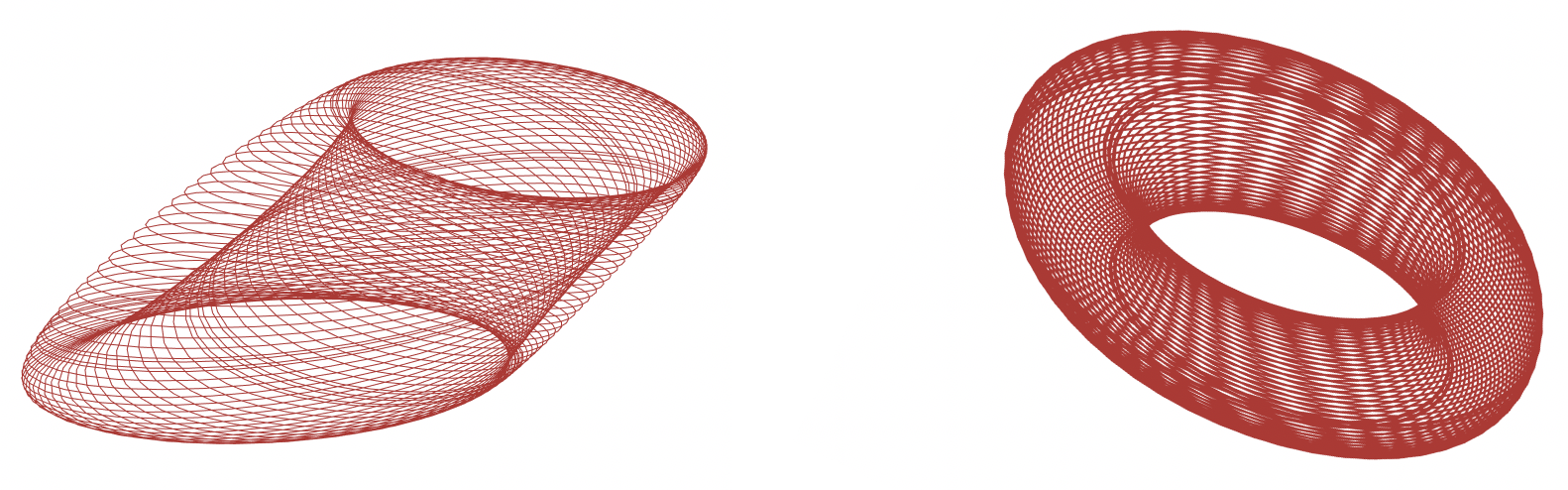
for suitable reals that depend on the initial position but not on . This again produces a two-dimensional attracting subset of formed by the Minkowski sum of two ellipses. In the case of Figure 8, the attractor is a torus pinched along two curves. The main difference from the previous case comes from the limit behavior of the agents. They are not attracted to a fixed point but, rather, to a surface. With high probability, the orbits are asymptotically periodic if is rational, and quasi-periodic otherwise. For a case of the former, consider , which gives us
hence periodic orbits.

2.5.3 Equidistribution over the attractor
Put and . We set . For any , we have
We verified numerically that and , where
By (12),
Computer experimentation points to the linear independence of the numbers over the rationals. If so, then Assumption 1 from Section 2.4 holds and, by Theorem 2.20, any limiting orbit is uniformly distributed over the attractor (Fig.9).

3 Dynamic Social Networks
We define a mixed model of contrarian opinion dynamics. Let be a set of nonempty subsets, each one spanning the vector space . At each time step , we define the matrix by choosing, as convolution set , a random, uniformly distributed element of . As before, we assume that . Let be the eigenvalue of associated with . Given an infinite sequence of indices from , we denote by be the first indices of , and we write . We generalize (4) into
| (16) |
where is the row vector .
3.1 Spectral decomposition
Write and ; because all the eigenvalues other than lie strictly inside the unit circle, we have . Without loss of generality, we can assume that . Indeed, suppose that ; then, for every , there is such that . This presents us with a “coupon collector’s” scenario: with probability at most , we have for at least one nonzero . In other words, with high probability, every coordinate of in the eigenbasis will vanish after steps; hence for all large enough. This case is of little interest, so we dismiss it and assume that is positive. We redefine . Let .
Lemma 3.1.
If is nonempty, there exists such that, with high probability, for all large enough,
Note that the high-probability event applies to all times larger than a fixed constant. The proof involves the comparison of two multiplicative random walks.
Proof 3.2.
Fix and . We prove that . If , then , for some . With high probability, the sequence includes the index at least once for any large enough; hence and the lemma holds. Assume now that ; for all , both of and are nonzero. Write , for , and note that , where . Let . The random variables are unbiased and mutually independent in . Classic deviation bounds [2] give us It follows that with probability , for an arbitrarily small constant . Since , it follows that, for arbitrarily small fixed and all large enough, with probability at least ,
for any given and . Setting and using a union bound completes the proof.
3.2 Surprising attractors
Adding mixing to a model increases the entropy of the system. It is thus to be expected that the attractor of a mixed model should have higher dimensionality than its pure components. The surprise is that this need not be the case. We exhibit instances of contrarian opinion dynamics where mixing decreases the dimension of the attractor. To keep the notation simple, we consider two pure models , alongside their mixture .
Theorem 3.3.
For any , there is a choice of and such that and ; in other words, the dimension of the mixture’s attractor can be arbitrarily smaller than those of its pure components.
Proof 3.4.
We define and , for any , where is the one-hot vector of whose -th coordinate is 1 and all the others 0. Let denote the set corresponding to the system . We easily verify that and , where is the inverse of in the field . A vector and its negative contribute to the same ellipse, so we have . We note that , for ; hence for and for all other values of . It follows that .
Figure 10 illustrates Theorem 3.3. We have and . The two convolution sets are and . The initial positions are random and identical in all three cases.

We can generalize the mixed model by picking (resp. ) with probability (resp. ), where . For this, we redefine and .
Theorem 3.5.
There is a choice of and such that ; in other words, the dimension of the mixture’s attractor can be larger than those of its pure components.
Proof 3.6.
Borrowing the notation of the previous proof, we define and and verify that and ; hence . Assuming that , we note that the sets and are disjoint. Regarding the mixed system, we have , where and . Around , we have, for all ,
| (18) |
Since , by continuity, there are and such that is equal to the right-hand side of (18). This implies that , which completes the proof.
Figure 11 illustrates the theorem. We have , , and . The two convolution sets are and ; the mixture probability is . The initial positions are random and identical in all three cases.

References
- [1] C. Fred Alford. Group Psychology and Political Theory. Yale University Press, 1994. URL: http://www.jstor.org/stable/j.ctt1dt007c.
- [2] Noga Alon and Joel H. Spencer. The Probabilistic Method, Third Edition. Wiley-Interscience series in discrete mathematics and optimization. Wiley, 2008.
- [3] Carmela Bernardo, Claudio Altafini, Anton Proskurnikov, and Francesco Vasca. Bounded confidence opinion dynamics: A survey. Automatica, 159:111302, 2024. URL: https://www.sciencedirect.com/science/article/pii/S0005109823004661, doi:https://doi.org/10.1016/j.automatica.2023.111302.
- [4] Arnab Bhattacharyya, Mark Braverman, Bernard Chazelle, and Huy L. Nguyen. On the convergence of the hegselmann-krause system. In Robert D. Kleinberg, editor, Innovations in Theoretical Computer Science, ITCS ’13, Berkeley, CA, USA, January 9-12, 2013, pages 61–66. ACM, 2013. URL: https://doi.org/10.1145/2422436.2422446, doi:10.1145/2422436.2422446.
- [5] Vincent D. Blondel, Julien M. Hendrickx, and John N. Tsitsiklis. On krause’s multi-agent consensus model with state-dependent connectivity. IEEE Trans. Autom. Control., 54(11):2586–2597, 2009. URL: https://doi.org/10.1109/TAC.2009.2031211, doi:10.1109/TAC.2009.2031211.
- [6] Alfred M. Bruckstein, Guillermo Sapiro, and Doron Shaked. Evolutions of planar polygons. Int. J. Pattern Recognit. Artif. Intell., 9(6):991–1014, 1995. URL: https://doi.org/10.1142/S0218001495000407, doi:10.1142/S0218001495000407.
- [7] J.W.S Cassels. An Introduction to Diophantine Approximation. Cambridge University Press, 1957.
- [8] Philips J. Davis. Circulant Matrices, volume 338. AMS Chelsea Publishing, 2nd edition, 1994.
- [9] Guillaume Deffuant, David Neau, Frédéric Amblard, and Gérard Weisbuch. Mixing beliefs among interacting agents. Adv. Complex Syst., 3(1-4):87–98, 2000. URL: https://doi.org/10.1142/S0219525900000078, doi:10.1142/S0219525900000078.
- [10] Morris H. DeGroot. Reaching a consensus. Journal of the American Statistical Association, 69(345):118–121, 1974. URL: http://www.jstor.org/stable/2285509.
- [11] Kaitlyn Eekhoff. Opinion formation dynamics with contrarians and zealots. SIAM J. Undergraduate Research Online, 12, 2019.
- [12] Adam N. Elmachtoub and Charles F. Van Loan. From random polygon to ellipse: An eigenanalysis. SIAM Rev., 52(1):151–170, 2010. URL: https://doi.org/10.1137/090746707, doi:10.1137/090746707.
- [13] Seyed Rasoul Etesami and Tamer Başar. Game-theoretic analysis of the hegselmann-krause model for opinion dynamics in finite dimensions. IEEE Trans. Autom. Control., 60(7):1886–1897, 2015. URL: https://doi.org/10.1109/TAC.2015.2394954, doi:10.1109/TAC.2015.2394954.
- [14] Fabio Fagnani and Paolo Frasca. Introduction to Averaging Dynamics over Networks, volume 472. Springer, 1st edition, 2018.
- [15] Henrique Ferraz de Arruda, Alexandre Benatti, Filipi Nascimento Silva, César Henrique Comin, and Luciano da Fontoura Costa. Contrarian effects and echo chamber formation in opinion dynamics. Journal of Physics: Complexity, 2(2):025010, mar 2021. URL: https://dx.doi.org/10.1088/2632-072X/abe561, doi:10.1088/2632-072X/abe561.
- [16] John R. P. French. A formal theory of social power. Psychological Review, 63(3):181–194, 1956. doi:10.1037/h0046123.
- [17] Noah E. Friedkin and Eugene C. Johnsen. Social influence and opinions. The Journal of Mathematical Sociology, 15(3-4):193–206, 1990. URL: https://doi.org/10.1080/0022250X.1990.9990069, doi:10.1080/0022250X.1990.9990069.
- [18] Serge Galam. From 2000 bush–gore to 2006 italian elections: voting at fifty-fifty and the contrarian effect. Quality & quantity, 41(4):579–589, 2007.
- [19] Serge Galam and Taksu Cheon. Asymmetric contrarians in opinion dynamics. Entropy, 22(1):25, 2020. URL: https://doi.org/10.3390/e22010025, doi:10.3390/E22010025.
- [20] Carl Heese. Information frictions and opposed political interests. American Economic Association, 2022.
- [21] Rainer Hegselmann and Ulrich Krause. Opinion dynamics and bounded confidence: models, analysis and simulation. J. Artif. Soc. Soc. Simul., 5(3), 2002. URL: http://jasss.soc.surrey.ac.uk/5/3/2.html.
- [22] Boyan Kostadinov. Limiting forms of iterated circular convolutions of planar polygons. International Journal of Applied and Computational Mathematics, 3:1779 – 1798, 2016.
- [23] L. Kuipers and H. Niederreiter. Uniform Distribution of Sequences. A Wiley-Interscience publication. Wiley, 1974.
- [24] Hsin-Min Lu. Detecting short-term cyclical topic dynamics in the user-generated content and news. Decis. Support Syst., 70:1–14, 2015. URL: https://doi.org/10.1016/j.dss.2014.11.006, doi:10.1016/J.DSS.2014.11.006.
- [25] Anders Martinsson. An improved energy argument for the hegselmann–krause model. Journal of Difference Equations and Applications, 22(4):513–518, 2016. doi:10.1080/10236198.2015.1115486.
- [26] Roni Muslim, M. Jauhar Kholili, and Ahmad R.T. Nugraha. Opinion dynamics involving contrarian and independence behaviors based on the sznajd model with two-two and three-one agent interactions. Physica D: Nonlinear Phenomena, 439:133379, 2022. URL: https://www.sciencedirect.com/science/article/pii/S0167278922001373, doi:https://doi.org/10.1016/j.physd.2022.133379.
- [27] E. Seneta. Non-negative Matrices and Markov Chains. Springer Series in Statistics. Springer, 2nd edition, 2006.